 Wenqian Jiang1
 Xiaoming Lin
- 1Metrology Center of Guangxi Power Grid Co., Ltd, Nanning, China
- 2Electric Power Research Institute, China Southern Power Grid Company Limited, Guangzhou, China
- 3Key Laboratory of Intelligent Measurement and Advanced Measurement Enterprises of Guangdong Power Grid, Guangzhou, China
The current residential electricity demand is increasing. The demand side response of smart grid power users aims to enable users to reasonably plan their own power consumption through price incentives, so as to solve the problems of unreasonable power energy structure and low utilization rate. It is prominent to mine the rules of user response behaviors and design a reasonable incentive mechanism to maximize the enthusiasm of all participants. The traditional demand response is to ensure the stability of the power system from the macro-control load of the grid, which cannot meet the personalized requirements of power users. The existing incentive mechanism also does not comprehensively consider the profits of grid companies, low-voltage users, aggregators and other parties. In this paper, we propose a user demand response framework based on load awareness. Firstly, we devise a user demand response behaviour model based on short-term memory network. Secondly, we propose a demand response incentive scheme based on electric power scores. We also construct a deviation optimization integration adjustment model based on game theory to achieve the balance of profits among grid, aggregators and low-voltage users. The extensive experimental results show the effectiveness of our proposed framework.
1 Introduction
Power energy is an important guarantee for achieving sustainable economic development and improving the quality of persons’ lives. At present, the increasing demand for residential electricity, coupled with the irrational structure and low utilization rate of existing power energy, have deepened the contradiction between the power load system and the distributed low-voltage grid users. In demand side response, during the peak or valley period of residential power consumption, users can reasonably plan their own power consumption range by means of price incentives and active response to the imbalance of regional power demand, thereby achieving peak shaving and valley filling to ensure the smooth operation of the grid. The implementation of demand response mechanism can realize power utilization optimization from the demand side of power resource allocation, effectively solve the problem of tight supply and demand of local power, and provide new regulation means for economic, safe and stable operation of the power system. The main current economic incentive is to determine the amount of subsidies according to the load data of demand response.
With the increasing types of power transactions and the increasing transaction frequency, the traditional power market transactions face more difficulties and challenges. With the development of new power integrated energy, especially the popularization of home photovoltaic new energy technology, the potential of low-voltage user demand response is enhanced. However, residential low-voltage users have their own particularity when participating in demand response. Specifically, the consumer’s electricity consumption behaviour will be affected by many factors such as season, weather temperature, power consumption period, and real-time price. It is necessary to build a user demand response model to reveal the degree of response of user power consumption to relevant change factors, and simulate the demand response behavior of users. On the other hand, it is necessary to design a reasonable incentive mechanism, so that the overall benefits and the individual benefits of all participants can be balanced, so as to maximize the enthusiasm of all participants.
The traditional demand response is to ensure the stability of the power system from the macro-control load of the grid. The grid system sends inductive signals to users to reduce load use, such as compensation and power price changes, so that users can change their original electricity use habits. However, the method of macro-control cannot meet the individual requirements of power users. With the increase of users participating in demand response, user responses are different and have various complex features such as high-dimensional, nonlinear, and non-convex. This makes the interactive modelling based on model driven and the pricing strategy based on optimization no longer applicable. Existing incentive mechanisms for power users are mainly launched from the electricity price, such as peak price, real-time price and electricity price rebates in response to peak hours, with reasonable subsidies and incentives. The common incentive method is point incentive, which can be used to exchange subsidies through the distribution of scores for users’ daily behaviours. This traditional method does not comprehensively consider the interests of power grid companies, low-voltage users, aggregators and other parties.
In this paper, we propose a user demand response framework based on load sensing to analyze the demand response behaviour of low-voltage users, and achieve effective incentives for grid companies, low-voltage users, aggregators and other agents. Specifically, we build a user participation demand response behaviour model to find out the correlation characteristics between the user’s electricity consumption and user’s behavior participating in demand response. We construct a theoretical model with a presentation layer, a user consumption prediction layer, a demand response prediction layer and a multi task learning layer.
Next, we design the integration rules of differential scoring mechanism under three objectives: maximizing the scores obtained by users, maximizing the benefits of grid companies, and maximizing the benefits of aggregators. We devise a market trading rules for low-voltage demand response including five stages of the trading process: demand response invitation, the bidding stage, the orderly power consumption stage, the photovoltaic new energy power sale stage, and the release and distribution of subsidy information stage. The integration rules of differential integral mechanism under three objectives are designed: maximizing the points obtained by users, maximizing the benefits of grid companies, and maximizing the benefits of aggregators.
Finally, we construct a deviation optimization score adjusting model, which comprehensively considers the real-time price of grid companies, the unit price of load dispatching of aggregators, and the demand response of low-voltage users. The score adjusting model simulates the implementation effect when the grid, aggregators, and low-voltage users participate in demand response. According to the deviation of implementation effect, the incentive mechanism of power integration is optimized and adjusted. We adopt the non-cooperative static game to describe the three parties’ game. The maximum of the objective function can be achieved according to the benefit function of each party, that is, to maximize the benefits of grid companies, aggregators and low-voltage users. Then, according to the obtained Nash equilibrium solution, the deviation of the goal in the score incentive mechanism is optimized and adjusted.
Our main contributions are as follows.
• We propose a user demand response framework based on load awareness. This framework realizes the demand response behaviour analysis of low-voltage users, and constructs an incentive mechanism based on grid companies, low-voltage users, aggregators and other parties.
• We propose a low-voltage user participation demand response behaviour model, which learns user behaviour via LSTM (long short-term memory) network.
• We devise the demand response incentive scheme based on electricity scoring. A deviation optimization integration adjustment model based on game theory is presented to simulate the implementation effect of grid, aggregator and low-voltage users.
• We conduct extensive experiments. The experimental results show the effectiveness of the proposed method.
The rest of this paper is structured as follows. We summarize the related work in Section 2. We present the user participation demand response behaviour theory model in Section 3. We present the demand response incentive scheme in Section 4. We discuss about the incentive adjustment model in Section 5. The experimental design and results are presented in Section 6. Finally, Section 7 presents the conclusion.
2 Related work
It is well known that demand response plays an important role in balancing supply and demand in the power sector. Wijaya et al. (2014) and Shi et al. (2020) demonstrated how user engagement changes based on actual incentives received. Aalami et al. (2008) considered time-of-use and emergency demand response program. Zheng et al. (2020) proposed an incentive-based integrated demand response model. Wang et al. (2020) proposed a forecasting model to help aggregators predict the aggregate demand response capacity available in the future market. Baboli et al. (2012) developed an improved demand response model which considers the customer’s behaviour. Muratori and Rizzoni (2016) provided an accurate estimate of the actual quantity of controllable resources. From the perspective of a grid operator, Yu et al. (2019) established a resource trading framework. Khajavi et al. (2011) and Palensky and Dietrich (2011) analyzed the incentive-based programs in smart grid and the various types of demand side management. Yang et al. (2018) provided different consumers with a list of price plans to motivate them to participate in demand response. Wang et al. (2020) constructed the automatic demand response architecture, which provides the possibility of demand response’s real-time application.
The relationships between entities in a dataset usually have multiple properties, and many methods using subspace weighted clustering and long short-term memory network have been proposed to analyze these attributes. Jia and Cheung (2018) proposed an attribute-weighted clustering model based on the concept of object-cluster similarity. Jing et al. (2007) proposed a new k-means algorithm that can cluster high-dimensional objects in sub-spaces. Boongoen et al. (2011) studied subspace clustering, and proposed a filter approach applicable to different types of clustering. Chen et al. (2019) proposed a two-level subspace weighting clustering algorithm for customer transaction data. Yin et al. (2018) proposed a clustering method, which learns an adaptive graph affinity matrix and then obviates the pre-computed graph regularize effectively. Tang et al. (2019) learned a joint affinity graph for multi-view subspace clustering. Dong et al. (2014) proposed a method to cluster the vertices by efficiently merging the information. Some studies used the LSTM (long short-term memory) network and RNN network for prediction (Xiaoyun et al., 2016; Liu et al., 2017; Narayan and Hipel, 2017; Agrawal et al., 2018).
In addition, there are some methods to apply game theory to smart grid. Nguyen et al. (2013) proposed a strategy to solve the conflict of interest to achieve the overall optimal performance of the power supply system. Sanjab and Saad (2016) and Kamyab et al. (2016) proposed a distributed learning algorithm to find the equilibrium and proved its convergence to the game solution. Belhaiza and Baroudi (2015) proposed a new non-cooperative game theory model. The Nash Balance condition is used for demand management in the smart grid. Farraj et al. (2016) uses an iterative game theory formula to describe the interaction of all parties in the power system and its impact on system stability. Ni and Paul (2019) proposed a new solution for the dynamic game between parties. Demand response algorithms based on real-time price are proposed in (Tushar et al., 2014; Mondal et al., 2015; Yu and Hong, 2016). Nguyen et al. (2015) proposed a distributed demand-side management algorithm, which provides optimality for energy suppliers and users. La et al. (2016) established a dynamic pricing model based on differential game theory. Fadlullah et al. (2014) proposed a game-theoretic energy schedule method by modeling the interaction between power companies and consumers.
Recently, Fu and Zhou (2022) proposed a preprocessing approach for the simulation of the power systems. A tranfer function model is proposed to evaluate the characteristics of droop control inverter. Some researches focus on new energy generation such as photovoltaic power generation. Specifically, Fu and Zhou (2022) addressed the problem of the collaboration between photovoltaic load and energy systems, in order to coordinate the energy, such as electrical energy and thermal energy. A energy meteorological model is constructed. Machine learning techniques, such as Markov chains, nearest neighbor theory and probabilistic inequality theory, are used for optimal planning for capacitors in (Fu et al., 2020). The statical machine learning is utilized for power flow planning in (Fu, 2022). The statical machine learning techniques contains linear regression, probability distribution, and center point method, which simulate the uncertain weather, power generation, and others.
3 User participation demand response behavior theory model in load regulation
By analyzing users’ historical electricity consumption behaviour, we can get their overall electricity consumption habits and characteristics, thus we can formulate electricity planning schemes that are more consistent with users’ behaviour habits and formulate relevant incentive policies. In daily life, there are many external factors that will affect the power consumption of users, such as season, weather temperature, power consumption period, and real-time price. Motivated by the multi-task learning model in Xu et al. (2021), we use the division of different time periods on the timeline to describe the impact of users’ historical electricity consumption behaviour on the future, and enhance the representation. For external features, we combine the context information of electricity consumption, and use LSTM to learn. Finally, combining the two data, more accurate results can be obtained through loss function calculation. Therefore, the whole user participation demand response behavior theoretical model is divided into four layers: expression layer, user consumption prediction layer, load prediction layer, and multi-task learning layer.
1) Expression Layer.
This layer is composed of external characteristics and user electricity consumption information. External features are the top n features extracted above. The selected features are coded into the vector of
2) User Consumption Forecast Layer.
This layer uses the user consumption amount to represent the consumption situation, and extracts the user consumption amount on the timeline. The time is divided into timeslots with a growth of t (for example, t = 5 (minutes)). We use Au,t to represent the average amount consumed by the user u in the timeslot t. We hope to use this value to predict the user consumption amount of
Convolution operations are performed on the three types of features as follows.
where * represents the convolution operation, and
3) User Demand Response Prediction Layer.
The purpose of designing the user demand response prediction layer is to predict the user participation demand response based on the sequence model of space-time information. LSTM network is used to retain useful information. In the LSTM network, each feature vector has a memory unit cx, an input gate ix and a forgetting gate fx that controls the network to remember useful new content and forget useless old content, and an output gate ox where x represents the xth feature vector. For each eigenvector, there is an output hx of LSTM unit: hx = ox◦tanh (cx). The output gate uses a Sigmod function to determine the output: ox = σ(WoUx,τ + Vohx−1+ Docx). Do is a diagonal matrix. The memory unit cx is obtained from the weighted sum of new content
Both Wc and Vc are weight matrices. The input gate and forgetting gate are calculated from the information Ux,τ, the output hx−1 of the last LSTM unit, and the last memory unit cx−1 connected by external features and user consumption related context:
where Wy, Wf, Vy, Vf are weight matrices, and Dy, Df are diagonal matrices. Using the sequence of Uj,τ to train the LSTM network, we can get the hidden unit sequence H = h1, h2, … , hn with time dependence. After this unit sequence is input into the MLP, the corresponding expected user participation demand response
In order to further capture the global information, we employ the self-attention mechanism and multi-task parallel computing, which can take into account the correlation between any two stations. The corresponding trainable parameter matrix
Each element in the Q sequence is used to match each element in K. Specifically, point multiplication is carried out between them in order to obtain the weight through softmax function. V can be regarded as the information learned from the sequence. Therefore, this process can be expressed as follows.
where dk represents the dimension of k, and h* represents the comprehensive representation of sequence H. h* will be input into MLP to obtain the final predicted user demand response
4) Multi-Task Learning Layer.
The purpose of this layer is to calculate more accurate parameters by combining the outputs of the user consumption prediction layer and the user demand response prediction layer. Using the predicted user consumption amount
4 Demand response incentive scheme based on electric score
For low-voltage users participating in demand response transactions, if they perform faithfully, they can accumulate credit value and reward scores. If users default, they will be punished. In this section, we develop a differential scoring model. The goal is to maximize the credit obtained by users and the income of grid companies and aggregators.
4.1 Score rules
1) Rewarding scores for user registration and real name authentication: After users download the low-voltage interactive response APP, register and authenticate with their real names, the system will reward users with scores, such as 20 scores.
2) The user submits the demand response information and gets bonus scores. After receiving the demand response invitation issued by the grid company, the user will submit relevant information according to the situation, and the system will issue reward scores to the user, such as 5 scores.
3) Rewarding scores for faithful performance of users. The aggregator compares the data read from the intelligent interactive terminal with the data submitted by the user. If the user performs faithfully, the system will give the user a performance award, such as 10 scores.
4) Deducting scores for user’s failure to perform. If the user breaches the contract, the user’s partial scores will be deducted, such as 15 scores.
5) Differentiated bonus scores are calculated according to the user’s credit value. The system sets a basic reward score, such as 12 scores, and then rewards according to the credit value. For users with high credit value (for example, above 900), each time they participate in a transaction and perform, they can be rewarded with the original bonus scores plus p times the original scores (for example, p = 0.2). For users with moderate credit value (500–900), each time they participate in a transaction and perform a contract, they can reward the original score plus q times the original score (for example, q = 0.05). Users with low credit value (below 500) will be rewarded normally.
6) User task credits: for a user’s time-limited task, for example, if he/she participates in 6 demand response transactions within half a month and performs faithfully, he/she can obtain 3 scores.
7) Rewards for blockchain block out: the block reward of the corresponding alliance chain of each station area is planned and managed by the grid company in a unified way and distributed to users according to their enthusiasm for participation.
8) Rewards for users to participate in orderly power consumption: after receiving the invitation, the user submits the transaction information, chooses to discharge the electric vehicle at the peak load and charge it at the low load, and the system will give the user a point reward, such as 18 scores.
9) Rewards for photovoltaic new energy sales: photovoltaic power generation users will voluntarily use the electricity and sell the surplus electricity to the grid. The grid company will give a point reward, such as 1 point for 1 kWh.
10) Bonus scores for users binding new smart home devices: users who bind a new smart home device through the APP will get bonus scores, such as 5 scores.
Users can use credits before the credits expire. Specifically, the purposes of scores include:
1) Exchange electricity subsidy price: users can convert it into electricity subsidy in proportion, for example, 500 scores can be converted into an electricity subsidy of 1 kW h, but it cannot be withdrawn for use.
2) Exchange souvenirs and prizes: for example, 2,000 cents can be exchanged for souvenirs, and 1,000 cents can be exchanged for vouchers of cooperative merchants, etc.
3) Restore credit value: for users with low credit value (for example, the credit value is lower than 200), credit value can be restored with scores.
4.2 Maximizing the user’s scores
We divide the sources of user scores into six parts. Let A be the sum of the scores obtained by each user’s daily behaviour, including reward scores registi,u obtained by user registration and real name authentication, reward scores submiti,u obtained by users submitting demand response information, user task scores taski,u, reward scores bindi,u for users binding new smart home devices, subscript i for station area number, and u for user code. Therefore, the sum of scores obtained by all users’ daily behaviours can be expressed as A, which can be expressed as follows.
Let B be the sum of the scores of each user’s participation in demand response performance, including the score caset of the predicted demand response reward. The performance score is differential. Users get different credits at different implementation times, which are differentiated by time factor τt. We use Hx to denote time, Dx to denote date, Mx to denote month, and q, w, r to denote weight coefficients respectively, which can be adjusted according to season, temperature and other factors. Therefore, the calculation method of time coefficient τt is:
We use X to denote the predicted user demand response, and θ to denote the reward basis for each kW hour of electricity, so the reward scores obtained by users are calculated as follows:
Therefore, the total score B of all users’ participation in demand response performance can be expressed as:
Then, according to the sum of the differentiated credits of the user credit value award, we use C to denote the credit value of the user. The user’s credit value is divided into three grades, expressed as grade factor δe, subscript e as user credit value, and credit value award base score as ρ. δe is calculated as follows.
The differentiation scores obtained by users are:
Therefore, the sum of differential scores C awarded according to the user’s credit value can be expressed as:
The block reward scores for blockchain are uniformly distributed and managed by the grid company. The scores are sorted from high to low according to the response of each station area and the response of users in the station area. The ranking coefficient of the substation area is expressed as αi, and i is the number of the station area. We use βu to denote the ranking coefficient of users in the station area, and u to represent the number of users in the station area. If the basic division is set as η, the user will get mineri bonus scores for block out as follows.
We use D to denote the total reward scores of all users’ blockchain blocks, and D can be obtained as follows.
We use E to denote the sum of the rewards for users to participate in the orderly use of electricity. orderi,u represents the scores obtained by each user to participate in the orderly use of electricity.
We use F to denote the total scores of energy sales incentives, and photovoltaici,u to denote the bonus scores obtained by each PV new energy user by selling excess electricity:
Therefore, the model for maximizing user scores is:
4.3 Maximizing profit of grid companies
We use SCSG to denote the revenue of the grid company. It refers to the total revenue after the end of the demand response load. Let a, b and c be the weight of demand response, orderly power consumption and photovoltaic new energy power generation in the whole low-voltage interaction response. There are three sources of demand response transaction load. We use Xi to denote a total load of demand response of the ith station area. We use Yi,u to denote the load of the uth user in the ith substation area who sells the load stored by the electric vehicle to other users to participate in demand response in the orderly power consumption stage. We use Zi,u to denote the excess load sold to the grid company by the user u of the ith station area in the photovoltaic power generation stage. Let pt be the real-time electricity selling price of the grid company in period p. Let pw be the dispatching load unit price of the aggregator, and let pc be the generation cost of the grid company. Therefore, the benefit maximization model of grid companies can be expressed as:
4.4 Maximizing aggregator’s profit
The aggregator participates in the process of dispatching demand response load, and the grid company pays the dispatching fee, which is represented by SAgent. The three expressions of the demand response load dispatched by the aggregator are denoted as Xi, Yi,u, Zi,u, Here, a, b and c are also used to represent the weight of demand response, orderly electricity use and photovoltaic new energy power generation in the whole low-voltage interaction response. Let pw be the unit price of the dispatching load charged by the aggregator for participating in the dispatching load. Therefore, the profit maximization model of aggregators can be expressed as:
The demand response incentive model based on electric score is feasible in reality. The power grid company will install a specific electricity meter in each user’s home. When users use the application program (such as mobile APP) that matches the electricity meter, they can become the client of the demand response system, that is, the light node in the blockchain system. The settlement of score is calculated by the whole node with large computing power in the blockchain system, and then synchronized to the user light node. When the application program that conforms to the business logic in the paper is completed, the power regulation and score settlement based on the blockchain system is very simple and fast for power grid companies, aggregators and low-voltage users.
5 Incentive adjustment model of scores based on game theory
We simulate the implementation effect of multi-agents’ participation in demand response based on game theory. We optimize and adjust the scoring incentive mechanism according to the target deviation of demand response. The game involving grid companies, aggregators and low-voltage users is a non-cooperative static game, and the three parties independently choose their strategies according to their own optimization goals. The optimization objectives of grid companies, aggregators, and low-voltage users are as follows: maximum benefits, maximum benefits from dispatching demand response, and maximum scores. According to the goal of the three party game, solve the Nash equilibrium point and adjust the score incentive mechanism.
5.1 Game model
The game model of the grid company, aggregator and low-voltage user is as follows:
Participants: grid company CSG, aggregator Agent, and all user Users participating in low voltage response.
Strategy: the game decision variables of grid company, aggregator and low voltage user include real-time unit price of load in demand response period, dispatch unit price of aggregator participating in dispatching demand response load, and demand response quantity submitted by low voltage users.
Profit:
SCSG denotes the total income of the grid company after the end of the demand response load. a, b and c are the weights of demand response, orderly power consumption and photovoltaic new energy power generation in the whole low-voltage interaction response. Xi refers to the total load of demand response of the ith substation area. Yi,u refers to the phase of orderly power utilization, in which the user u of the ith substation sells the load stored by the electric vehicle itself to other users to participate in demand response. Zi,u refers to the excess load sold to the grid company by the user u of the ith substation in the photovoltaic power generation stage. pt refers to the real-time electricity selling price of the grid company in the p period. pw refers to the unit price of dispatching load of the aggregator. pc refers to the generation cost of the grid company. Eq. 38 scores out that the optimization objective of the aggregator is to obtain the maximum benefit in the process of participating in dispatching demand response load. pw refers to the unit price of dispatching load charged by the aggregator for participating in dispatching load. Eq. 39 scores out that the optimization goal of low-voltage users is to maximize the integration. A, C, D, E, and F refer to the fixed scores obtained by users under different circumstances.
5.2 Tripartite game
5.2.1 Grid companies increase unit price of real-time load
1) The aggregator chooses to increase the unit price of the dispatching load, and the user chooses to increase the demand response load.
The total electric power scores obtained by the user, the income obtained by the grid company, and the income obtained by the aggregators are as follows.
2) The aggregator chooses to increase the unit price of the dispatching load, and the user chooses to reduce the demand response load.
The total electric power scores obtained by the user, the income obtained by the grid company, and the income obtained by the aggregators are as follows.
3) The aggregator chooses to reduce the unit price of the dispatching load, and the user chooses to increase the demand response load.
The total electric power scores obtained by the user, the income obtained by the grid company, and the income obtained by the aggregator are as follows.
4) The aggregator chooses to reduce the unit price of the dispatching load, and the user chooses to reduce the response load.
The total electric power scores obtained by the user, the income obtained by the grid company, and the income obtained by the aggregator are as follows.
5.2.2 Grid companies reduce unit price of real-time power load
1) The aggregator chooses to increase the unit price of the dispatching load, and the user chooses to increase the demand response load.
The total electric power scores obtained by the user, the income obtained by the grid company, and the income obtained by the aggregator are as follows.
2) The aggregator chooses to increase the unit price of the dispatching load, and the user chooses to reduce the demand response load.
The total electric power scores obtained by the user, the income obtained by the grid company, and the income obtained by the aggregator are as follows.
3) The aggregator chooses to reduce the unit price of the dispatching load, and the user chooses to increase the demand response load.
The total electric power scores obtained by the user, the income obtained by the grid company, and the income obtained by the aggregator are as follows.
4) The aggregator chooses to reduce the unit price of the dispatching load, and the user chooses to reduce the response load.
The total electric power scores obtained by the user, the income obtained by the grid company, and the income obtained by the aggregator are as follows.
According to the independent optimization objectives of the three parties in the game, all strategy sets are simultaneously traversed to solve the Nash equilibrium. The specific implementation ideas are as follows: initializing all parameters required for modeling, going through all game strategies and calculate the income function, judging whether to find Nash equilibrium according to the definition, and analyzing the output Nash equilibrium solution.
Finally, the grid company optimizes the score incentive mechanism according to the Nash equilibrium solution. Grid companies set corresponding real-time electricity prices, while aggregators adjust corresponding dispatch costs, low-voltage users make the total submitted demand response the corresponding Nash balance strategy. This adjustment process is different from the previous grid companies’ mode of selling electricity and purchasing electricity by users. Grid companies will increase real-time prices during peak hours of power consumption, which will encourage users to participate in more demand-response transactions to ease the generation pressure during peak hours of power consumption. At the same time, during the peak period of power consumption, grid companies will reduce the real-time price, which will enable users to participate in the normal use of power, thus narrowing the gap between power peaks and valleys.
5.3 Discussion
We now discuss about the application of the proposed methods in practical projects. The user participation demand response behaviour theory model in load regulation predicts the future user consumption behaviour through the analysis of existing low-voltage user power consumption data. In practice, it is convenient for the grid company to predict the total power consumption load of low-voltage users at any time in the future, and combine the peaks and troughs of the entire grid system load to carry out macro regulation, Thus, the electricity price of various power users in different periods can be arranged more reasonably.
The demand response incentive scheme based on electric score aims to stimulate users’ initiative and carry out load exchange independently. In practical applications, each user can be regarded as a node participating in power storage and consumption in the power grid. When each node participates in load regulation according to the incentive mechanism, the load curve of the power grid will become more stable, operate more safely and benefit more.
The incentive adjustment model of scores based on game theory is simulated by game theory. When the above demand response incentive mechanism is operated, the benefits of the game between the grid company, aggregators and low-voltage users can be obtained. In practical application, continuous deviation optimization and adjustment of the integration mechanism based on the tripartite benefits can make the incentive model more reasonable, user participation higher, form a virtuous cycle, and build a stable load regulation ecology.
Moreover, the proposed demand-side response framework can absorb new energy generation such as photovoltaic power generation, because the power can come from photovoltaic new energy (as stated in Section 4).
6 Evaluation
6.1 Experiment of demand response user behaviour analysis
The experimental settings are shown in Table 1. We use synthetic datasets. The size of the data set of the user consumption layer is 300 * 100, representing 300 users and the user consumption data of 100-time gaps. User consumption data are randomly generated in the range [0.5, 5.5]. The size of the data set of the demand response prediction layer is 300 * 8, representing 300 station areas. There are five external features which are random values in [0, 30]. There are also three convolved features with user consumption-related time characteristics, that is, the hidden layer, which respectively represents the user consumption characteristics of three different cycles. The cycle is divided into 7 days, 15 days, and 30 days. They are then convolved in order to efficiently process the temporal information and get the temporal relationship. It can also extract the temporal features like the convolutional layer to get the hidden user consumption features of three types of cycles. In the demand response prediction layer, all the information obtained from the expression layer is concatenated as input, and the LSTM model is used to obtain the hidden unit sequences containing time dependence. Considering the spatial characteristics, that is, the correlation between stations, the self-attention mechanism is used for these sequences. In the multi-task learning layer, based on the predicted values obtained in the first three layers (i.e., the predicted amount of the user consumption layer, the predicted response values, and space characteristics in the response prediction layer), iterative training is conducted to minimize the loss function.

TABLE 1. Experimental settings (Demand response user behaviour analysis).
We compare our Ml-PDRM (multi-task user participation demand response behaviour) approach with LSTM and LSTM + CNN to predict the response. LSTM network can integrate the characteristics of external features in time series. The LSTM + CNN algorithm can integrate the consumption amount characteristics and external features of users in different periods.
We measure the predicted response of each algorithm with the actual response. We also measure the average absolute error MAE, which represents the average of the absolute error between the predicted value and the observed value. In the experiment, the observed value is the actual response, and the predicted value is the user demand response predicted by the algorithm.
The experiment was run on the Google platform, with a memory of 128GB, the operating system of Ubuntu 18.04.6 LTS, and the programming language of python. The Python version is 3.7.14, the Cuda version is 11.1, and the TensorFlow version is 2.8.2.
Figure 1 shows the comparison results on the predicted response of the three algorithms, i.e., the actual response when the prediction time is 1, 2, 3, 5, 8, and 10 respectively. Taking Figure 1A as an example, when the prediction time is equal to 1 and the period is 29, the actual response is 21.03, the response predicted by Mul-PDRM is 20.93, the response predicted by LSTM + CNN is 20.25, and the response volume predicted by LSTM is 20.13. From the perspective of prediction time, with the increase of prediction time, the deviation between the predicted response quantity of the three algorithms and the actual value will become larger and larger. Compared with the other two algorithms, the predicted response of Mul-PDRM model is more consistent with the actual response, and the trend is more consistent.
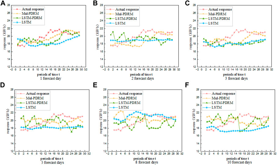
FIGURE 1. Predicted response vs actual response.
Figure 2 shows the influence of different prediction days and algorithms on the average absolute error after response prediction. Taking Figure 2A as an example, when the number of days to predict is 1, the average absolute error of Mul-PDRM algorithm is 0.82, the average absolute error of LSTM + CNN algorithm is 1.73, and the average absolute error of LSTM algorithm is 1.83. It can be seen that with the increase of forecast days, the average absolute error of Mul-PDRM algorithm will increase correspondingly, and the average absolute error of LSTM + CNN and LSTM algorithm will fluctuate and increase. We can see that the average absolute error of LSTM-PDRM algorithm in predicting the response is smaller than that of LSTM + CNN and LSTM algorithms, which means that the results are more accurate and the prediction is more reliable.
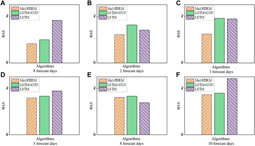
FIGURE 2. Average absolute error MAE (A) Algorithms 8 forecast days (B) Algorithms 2 forecast days (C) Algorithms 3 forecast days (D) Algorithms 5 forecast days (E) Algorithms 8 forecast days (F) Algorithms 10 forecast days.
From the experimental results, compared with the other two algorithms, the response predicted by Mul-PDRM algorithm is the most consistent with the actual response. The average absolute error of Mul-PDRM algorithm is also smaller than the other two algorithms. Therefore, it can be concluded that Mul-PDRM algorithm has improved the accuracy of prediction results compared with the comparison algorithm. At the same time, the error of MUR-PDRM algorithm in predicting the response will be larger with the increase of the prediction time, so it is more suitable for predicting the short-term user demand response.
6.2 Game theory experiments
Experimental settings. We use synthetic datasets where the parameter settings of experiments are shown in Table 2. The unit price of power load on the grid side is randomly generated in [0.2, 0.5]. The response quantity on the user side is randomly generated in [800, 1000]. The dispatching unit price on the aggregator side is randomly generated in [0.2, 0.5]. The initial income or score of users, grid companies and aggregators is set to 0. We did not consider the impact of orderly electricity use and photovoltaic new energy power generation in user income on the game theory process of user participation in demand response. So the weight of both is set to 0 and the weight of demand response is set to 1.
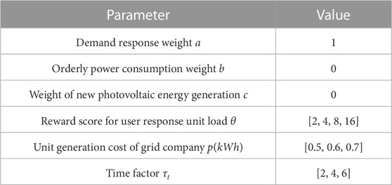
TABLE 2. Setting of experimental data.
The possibility of selecting the corresponding strategy is represented by a probability array [x, y], where x and y are decimals less than 1. x represents the probability that the player selects strategy 1, and y represents the probability that the player selects strategy 2. When x > y, it means that the player will choose strategy 1; when x < y, it means that the player will choose strategy 2. In each game process, three groups of probability arrays will be generated to represent the probability of the three players participating in the game.
We measure the effect of time coefficients, reward scores and the power generation cost, respectively. In the time coefficient experiment, we set the reward score of user response to unit load to 2, and set the unit power generation cost of grid company to 0.63 kW⋅ h. According to the two decisions of users, grid companies, and aggregators in the game model, we calculate the payoff matrix, and compare the convergence of income in the process of simulating tripartite transactions under different time coefficient settings. In the reward score experiment, the time coefficient is set to 2. The unit power generation cost of the grid company is set to 0.63 kW⋅ h, in order to simulate the tripartite transaction process when different users respond to the reward score of unit load. In the power generation cost experiment, we set the reward score to 2. We set the time coefficient of the user’s response to the unit load to 2. We simulate the tripartite transaction process when the unit power generation cost of the grid company is different.
Effect of time coefficient. Players 1, 2, and 3 represent users, grids and aggregators respectively. Through the model of adjusting the score incentive mechanism based on the tripartite game, we can get that the two strategies of the power grid are to increase the unit price of real-time power load and reduce the unit price of real-time power load. The two strategies of users are to increase the response volume and reduce the response volume. The two strategies of aggregators are to increase the scheduling unit price and reduce the scheduling unit price. According to the income algorithm in the game model, the three-party pay-off matrices under different time coefficients are calculated respectively. We simulate the game process. Then, the three groups of probability matrices can be obtained, as shown in Table 3.
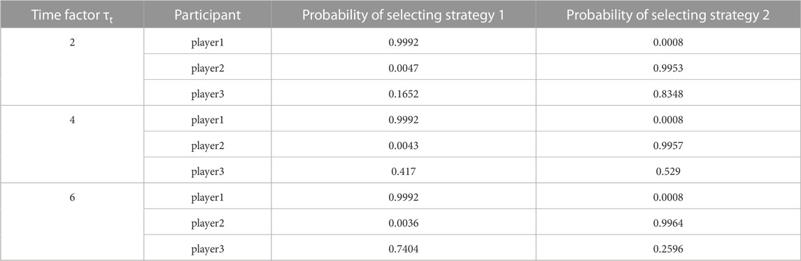
TABLE 3. Effect of time coefficients.
The experimental results are shown in Table 3. Taking the time coefficient of 2 as an example, for low-voltage load users, the probability of selecting strategy 1 is 0.9992, and the probability of selecting strategy 2 is 0.0008. For grid companies, the probability of selecting strategy 1 is 0.0047, and the probability of selecting strategy 2 is 0.9953. For aggregators, the probability of selecting strategy 1 is 0.1652, and the probability of selecting strategy 2 is 0.8348. It can be seen from the experimental results that when the time coefficient is set to 2, users will choose to improve the response, the grid will choose to reduce the unit price of real-time power load, and the aggregator will choose to reduce the unit price of dispatching. When the time factor is set to 4, the user will choose to increase the response, the grid will choose to reduce the unit price of real-time power load, and the aggregator will choose to reduce the dispatching unit price. When the time factor is set to 6, users will choose to improve the demand response, the grid will choose to reduce the real-time power consumption to meet the unit price, and the aggregator will choose to increase the dispatching unit price.
Effect of power generation cost. The experimental results are shown in Table 4. Taking the unit power generation cost of the power grid as an example, for low-voltage load users, the probability of selecting strategy 1 is 0.9992, and the probability of selecting strategy 2 is 0.0008. For grid companies, the probability of selecting strategy 1 is 0.0024, and the probability of selecting strategy 2 is 0.9976. For aggregators, the probability of selecting strategy 1 is 0.2821, and the probability of selecting strategy 2 is 0.7179. According to the score incentive mechanism model of the tripartite game, the experimental results show that when the unit power generation cost of the grid is 0.5 kW⋅ h, users are more inclined to choose to improve the demand response, the grid will choose to reduce the unit price of real-time power load, and the aggregator will choose to reduce the dispatching unit price. When the unit power generation cost of the grid company is 0.6 kW⋅ h, the user will choose to improve the demand response, the grid company will choose to reduce the unit price of real-time power load, and the aggregator will choose to increase the dispatching unit price. When the unit power generation cost of the grid company is 0.7 kW⋅ h, the user will choose to improve the demand response, the grid company will choose to reduce the unit price of power load, and the aggregator will choose to reduce the dispatching unit price.
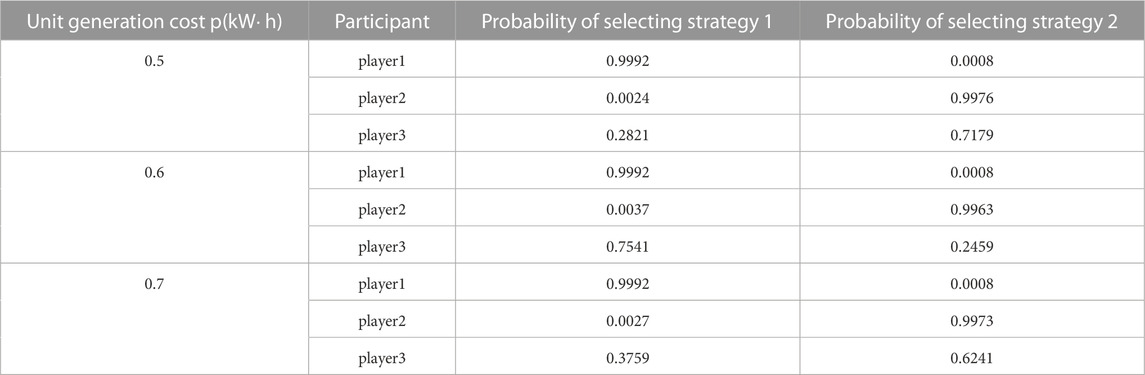
TABLE 4. Effect of power generation cost.
Effect of reward scores. The experimental results are shown in Table 5. Taking the unit load reward score of 2 as an example, for mortgage users, the probability of selecting strategy 1 is 0.9992, and the probability of selecting strategy 2 is 0.0008. For grid companies, the probability of selecting strategy 1 is 0.0032, and the probability of selecting strategy 2 is 0.9968. For aggregators, the probability of selecting strategy 1 is 0.5667, and the probability of selecting strategy 2 is 0.4333. By comparing the probability of participants choosing strategy 1 or 2, we can draw the following conclusions: when the unit load reward scores are 2, 4, 8, and 16, low-voltage users will choose to improve the response, the grid company will choose to reduce the unit price of real-time power load, and the aggregator will choose to increase the dispatching unit price.
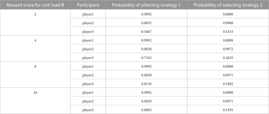
TABLE 5. Game results when the reward score for unit load is 2, 4, 8, and 16.
By simulating the game process of each group, we find the Nash equilibrium point and obtain the probability matrix of each group, so as to obtain the strategy choices of the parties involved in the game. The Nash equilibrium solution is combined with the actual situation, such as the user response, the unit price of the real-time power load of the grid company, and the dispatching unit price of the aggregator. It is proved that the power grid company can optimize and adjust the deviation of the score formula in the incentive integration mechanism, thereby achieving the goal of peak shaving and valley filling.
7 Conclusion
By analyzing the behavior characteristics of users’ electricity consumption and participation in demand response, we have built a theoretical model of user participation demand response behavior to predict the response of users. We have constructed the demand response incentive model based on power scores, and the differential scoring model for low-voltage demand response. Considering the implementation time, target, subsidy price and other factors, the profits of users, grid companies and load aggregators are maximized. Finally, we have used game theory to simulate the implementation effect of multi agents’ participation in demand response. A three-party game model is built based on the Nash equilibrium so as to optimize the score incentive mechanism.
Data availability statement
The original contributions presented in the study are included in the article/Supplementary Material, further inquiries can be directed to the corresponding author.
Author contributions
WJ, XL, and ZY contributed to conception and design of the study. JT, KZ, MZ, and YX organized the database and performed the statistical analysis. All authors contributed to manuscript writing, revision, and approved the submitted version. All authors listed have made a substantial, direct, and intellectual contribution to the work and approved it for publication.
Funding
This work was supported by the Science and Technology Project of Guangxi Power Grid Co., Ltd (044400KK52200003).
Acknowledgments
The authors would like to thank all of the people who participated in the studies.
Conflict of interest
Authors WJ, ZY and KZ were employed by Metrology Center of Guangxi Power Grid Co., Ltd. XL, JT, MZ and YX were employed by China Southern Power Grid Company Limited.
The authors declare that this study received funding from the Science and Technology Project of Guangxi Power Grid Co., Ltd. The funder had the following involvement in the study: data survey.
Publisher’s note
All claims expressed in this article are solely those of the authors and do not necessarily represent those of their affiliated organizations, or those of the publisher, the editors and the reviewers. Any product that may be evaluated in this article, or claim that may be made by its manufacturer, is not guaranteed or endorsed by the publisher.
References
Aalami, H., Yousefi, G. R., and Parsa Moghadam, M. (2008). “Demand response model considering edrp and tou programs,” in 2008 IEEE/PES transmission and distribution conference and exposition, 1–6. doi:10.1109/TDC.2008.4517059
Agrawal, R. K., Muchahary, F., and Tripathi, M. M. (2018). “Long term load forecasting with hourly predictions based on long-short-term-memory networks,” in 2018 IEEE Texas power and energy conference (TPEC), 1–6. doi:10.1109/TPEC.2018.8312088
Baboli, P. T., Eghbal, M., Moghaddam, M. P., and Aalami, H. (2012). “Customer behavior based demand response model,” in 2012 IEEE power and energy society general meeting (IEEE), 1–7.
Belhaiza, S., and Baroudi, U. (2015). A game theoretic model for smart grids demand management. IEEE Trans. Smart Grid 6, 1386–1393. doi:10.1109/TSG.2014.2376632
Boongoen, T., Shang, C., Iam-On, N., and Shen, Q. (2011). Extending data reliability measure to a filter approach for soft subspace clustering. IEEE Trans. Syst. Man, Cybern. Part B Cybern. 41, 1705–1714. doi:10.1109/TSMCB.2011.2160341
Chen, X., Sun, W., Wang, B., Li, Z., Wang, X., and Ye, Y. (2019). Spectral clustering of customer transaction data with a two-level subspace weighting method. IEEE Trans. Cybern. 49, 3230–3241. doi:10.1109/TCYB.2018.2836804
Dong, X., Frossard, P., Vandergheynst, P., and Nefedov, N. (2014). Clustering on multi-layer graphs via subspace analysis on grassmann manifolds. IEEE Trans. Signal Process. 62, 905–918. doi:10.1109/TSP.2013.2295553
Fadlullah, Z. M., Quan, D. M., Kato, N., and Stojmenovic, I. (2014). Gtes: An optimized game-theoretic demand-side management scheme for smart grid. IEEE Syst. J. 8, 588–597. doi:10.1109/JSYST.2013.2260934
Farraj, A., Hammad, E., Daoud, A. A., and Kundur, D. (2016). A game-theoretic analysis of cyber switching attacks and mitigation in smart grid systems. IEEE Trans. Smart Grid 7, 1846–1855. doi:10.1109/TSG.2015.2440095
Fu, X., Guo, Q., and Sun, H. (2020). Statistical machine learning model for stochastic optimal planning of distribution networks considering a dynamic correlation and dimension reduction. IEEE Trans. Smart Grid 11, 2904–2917. doi:10.1109/tsg.2020.2974021
Fu, X. (2022). Statistical machine learning model for capacitor planning considering uncertainties in photovoltaic power. Prot. Control Mod. Power Syst. 7, 5. doi:10.1186/s41601-022-00228-z
Fu, X., and Zhou, Y. (2022). Collaborative optimization of pv greenhouses and clean energy systems in rural areas. IEEE Trans. Sustain. Energy 14, 642–656. doi:10.1109/tste.2022.3223684
Jia, H., and Cheung, Y.-M. (2018). Subspace clustering of categorical and numerical data with an unknown number of clusters. IEEE Trans. Neural Netw. Learn. Syst. 29, 3308–3325. doi:10.1109/TNNLS.2017.2728138
Jing, L., Ng, M. K., and Huang, J. Z. (2007). An entropy weighting k-means algorithm for subspace clustering of high-dimensional sparse data. IEEE Trans. Knowl. Data Eng. 19, 1026–1041. doi:10.1109/TKDE.2007.1048
Kamyab, F., Amini, M., Sheykhha, S., Hasanpour, M., and Jalali, M. M. (2016). Demand response program in smart grid using supply function bidding mechanism. IEEE Trans. Smart Grid 7, 1277–1284. doi:10.1109/TSG.2015.2430364
Khajavi, P., Abniki, H., and Arani, A. B. (2011). “The role of incentive based demand response programs in smart grid,” in 2011 10th International Conference on Environment and Electrical Engineering, 1–4. doi:10.1109/EEEIC.2011.5874702
La, Q. D., Chan, Y. W. E., and Soong, B.-H. (2016). Power management of intelligent buildings facilitated by smart grid: A market approach. IEEE Trans. Smart Grid 7, 1389–1400. doi:10.1109/TSG.2015.2477852
Liu, C., Jin, Z., Gu, J., and Qiu, C. (2017). “Short-term load forecasting using a long short-term memory network,” in 2017 IEEE PES innovative smart grid technologies conference europe (ISGT-Europe), 1–6. doi:10.1109/ISGTEurope.2017.8260110
Mondal, A., Misra, S., and Obaidat, M. S. (2015). Distributed home energy management system with storage in smart grid using game theory. IEEE Syst. J. 11, 1857–1866. doi:10.1109/jsyst.2015.2421941
Muratori, M., and Rizzoni, G. (2016). Residential demand response: Dynamic energy management and time-varying electricity pricing. IEEE Trans. Power Syst. 31, 1108–1117. doi:10.1109/TPWRS.2015.2414880
Narayan, A., and Hipel, K. W. (2017). “Long short term memory networks for short-term electric load forecasting,” in 2017 IEEE Int. Conf. Syst. Man, Cybern. (SMC), 2573. –2578. doi:10.1109/SMC.2017.8123012
Nguyen, H. K., Song, J. B., and Han, Z. (2015). Distributed demand side management with energy storage in smart grid. IEEE Trans. Parallel Distributed Syst. 26, 3346–3357. doi:10.1109/TPDS.2014.2372781
Nguyen, P. H., Kling, W. L., and Ribeiro, P. F. (2013). A game theory strategy to integrate distributed agent-based functions in smart grids. IEEE Trans. Smart Grid 4, 568–576. doi:10.1109/TSG.2012.2236657
Ni, Z., and Paul, S. (2019). A multistage game in smart grid security: A reinforcement learning solution. IEEE Trans. Neural Netw. Learn. Syst. 30, 2684–2695. doi:10.1109/TNNLS.2018.2885530
Palensky, P., and Dietrich, D. (2011). Demand side management: Demand response, intelligent energy systems, and smart loads. IEEE Trans. Industrial Inf. 7, 381–388. doi:10.1109/TII.2011.2158841
Sanjab, A., and Saad, W. (2016). Data injection attacks on smart grids with multiple adversaries: A game-theoretic perspective. IEEE Trans. Smart Grid 7, 2038–2049. doi:10.1109/TSG.2016.2550218
Shi, Q., Chen, C.-F., Mammoli, A., and Li, F. (2020). Estimating the profile of incentive-based demand response (ibdr) by integrating technical models and social-behavioral factors. IEEE Trans. Smart Grid 11, 171–183. doi:10.1109/TSG.2019.2919601
Tang, C., Zhu, X., Liu, X., Li, M., Wang, P., Zhang, C., et al. (2019). Learning a joint affinity graph for multiview subspace clustering. IEEE Trans. Multimedia 21, 1724–1736. doi:10.1109/TMM.2018.2889560
Tushar, W., Zhang, J. A., Smith, D. B., Poor, H. V., and Thiébaux, S. (2014). Prioritizing consumers in smart grid: A game theoretic approach. IEEE Trans. Smart Grid 5, 1429–1438. doi:10.1109/TSG.2013.2293755
Wang, B., Li, Y., Ming, W., and Wang, S. (2020a). Deep reinforcement learning method for demand response management of interruptible load. IEEE Trans. Smart Grid 11, 3146–3155. doi:10.1109/TSG.2020.2967430
Wang, F., Xiang, B., Li, K., Ge, X., Lu, H., Lai, J., et al. (2020b). Smart households’ aggregated capacity forecasting for load aggregators under incentive-based demand response programs. IEEE Trans. Industry Appl. 56, 1086–1097. doi:10.1109/TIA.2020.2966426
Wijaya, T. K., Vasirani, M., and Aberer, K. (2014). When bias matters: An economic assessment of demand response baselines for residential customers. IEEE Trans. Smart Grid 5, 1755–1763. doi:10.1109/TSG.2014.2309053
Xiaoyun, Q., Xiaoning, K., Chao, Z., Shuai, J., and Xiuda, M. (2016). “Short-term prediction of wind power based on deep long short-term memory,” in 2016 IEEE PES asia-pacific power and energy engineering conference (APPEEC), 1148–1152. doi:10.1109/APPEEC.2016.7779672
Xu, J., Xu, S., Zhou, R., Liu, C., Liu, A., and Zhao, L. (2021). Taml: A traffic-aware multi-task learning model for estimating travel time. ACM Trans. Intelligent Syst. Technol. (TIST) 12, 1–14. doi:10.1145/3466686
Yang, H., Zhang, J., Qiu, J., Zhang, S., Lai, M., and Dong, Z. Y. (2018). A practical pricing approach to smart grid demand response based on load classification. IEEE Trans. Smart Grid 9, 179–190. doi:10.1109/TSG.2016.2547883
Yin, M., Xie, S., Wu, Z., Zhang, Y., and Gao, J. (2018). Subspace clustering via learning an adaptive low-rank graph. IEEE Trans. Image Process. 27, 3716–3728. doi:10.1109/TIP.2018.2825647
Yu, M., Hong, S. H., and Chan, B. K. K. (2016). A real-time demand-response algorithm for smart grids: A stackelberg game approach. IEEE Trans. Smart Grid 7, 1–20. doi:10.3897/zookeys.571.6894
Yu, M., Hong, S. H., Ding, Y., and Ye, X. (2019). An incentive-based demand response (dr) model considering composited dr resources. IEEE Trans. Industrial Electron. 66, 1488–1498. doi:10.1109/TIE.2018.2826454
Keywords: smart grid, behaviour characteristics, incentive mechanism, game theory, score adjusting
Citation: Jiang W, Lin X, Yang Z, Tang J, Zhang K, Zhou M and Xiao Y (2023) An efficient user demand response framework based on load sensing in smart grid. Front. Energy Res. 11:1141374. doi: 10.3389/fenrg.2023.1141374
Received: 11 January 2023; Accepted: 05 May 2023;
Published: 17 May 2023.
Edited by:
Yujian Ye, Southeast University, ChinaReviewed by:
Xueqian Fu, China Agricultural University, ChinaRui Wang, Northeastern University, China
Copyright © 2023 Jiang, Lin, Yang, Tang, Zhang, Zhou and Xiao. This is an open-access article distributed under the terms of the Creative Commons Attribution License (CC BY). The use, distribution or reproduction in other forums is permitted, provided the original author(s) and the copyright owner(s) are credited and that the original publication in this journal is cited, in accordance with accepted academic practice. No use, distribution or reproduction is permitted which does not comply with these terms.
*Correspondence: Xiaoming Lin, NDExODMzMjE0QHFxLmNvbQ==