Learning new attack vectors from misuse cases with deep reinforcement learning

Modern smart grids already consist of various components that interleave classical Operational Technology (OT) with Information and Communication Technology (ICT), which, in turn, have opened the power grid to advanced approaches using distributed software systems and even Artificial Intelligence (AI) applications. This IT/OT integration increases complexity, however, without argument, this advance is necessary to accommodate the rising numbers of prosumers, Distributed Energy Resources (DERs), to enable new market concepts, and to tackle world-wide CO₂ emission goals. But the increasing complexity of the Critical National Infrastructure (CNI) power grid gives way to numerous new attack vectors such that a priori robustness cannot be guaranteed anymore and run-time resilience, especially against the “unknown unknowns”, is the focus of current research. In this article, we present a novel combination of so called misuse-case modelling and an approach based on Deep Reinforcement Learning (DRL) to analyze a power grid for new attack vectors. Our approach enables learning from domain knowledge (offline learning), while expanding on that knowledge through learning agents that eventually uncover new attack vectors.

1 Introduction

Undoubtedly, the climate catastrophe is an unparalleled challenge for society. The urge to reduce CO₂ emissions directly leads to the imperative of reducing energy consumption, a more efficient usage of energy, and to increase the emount of renewable energy resources. This change is nowhere as apparent as in the power grid, which has undergone a rapid transformation in recent years (Bush, 2014; IEA, 2019).

Future power grids will have a much higher degree of digitalization as present ones. New approaches to balancing services management that include major prosumers (Holly et al., 2020) or multi-purpose battery storage (Tiemann et al., 2022). Multi-Agent System (MAS) are employed to facilitate real power management of DERs or solve unit-commitment problems (Roche et al., 2013; Veith, 2017; Nair et al., 2018; Frost et al., 2020; Mahela et al., 2022), while ever smaller generators are included into the grid management duties of the operator (Woltmann and Kittel, 2022). In addition, the convergence between Information Technology (IT) and OT is further emphasized by the amount of Internet of Things (IoT) technologies deployed, which have—for the better or worse—a huge impact on the power grid (Soltan et al., 2018; Huang et al., 2019; Mathas et al., 2021).

Indeed, power grids have become valuable targets for cyber attacks. The attacks on the Ukrainian power grid in 2015 and 2016 are well known (Styczynski and Beach-Westmoreland, 2016), but researchers know a multitude of attack vectors, such as message spoofing in IEC 61805 (Hong et al., 2014), false data injection (Liu et al., 2011; Hu et al., 2018), direct damage caused by nodes compromised by an attacker (Ju and Lin, 2018), or market exploitation (Wolgast et al., 2021). There are already comprehensive reviews available that consider the cyber-security of power grids; we refer the interested reader to the review article by Sun et al. (2018) for a comprehensive survey.

Researchers have not only considered each incident in isolation, but used and extended existing methodologies to document, classify, and analyze these incidents on a more general level. Structured Threat Information Expression (STIX) and Trusted Automated Exchange of Indicator Information (TAXII) are well-known documentation formats and methodologies for Cyber Threat Intelligence (CTI) (Barnum, 2012; Connolly et al., 2014; Apoorva et al., 2017; Briliyant et al., 2021). They are, of course, far from being the silver bullet; another, high-level approach is that of the Misuse-Case (MUC), introduced by Sindre and Opdahl (2005).

However, any approach in modelling cyber threats works based on already known attack vectors. They require humans to map them to actual actions—e. g, commands to be executed—on a given system, and it is also humans who devise and execute new attack vectors, which are then documented and analyzed post hoc.

There exists a stark contrast to more recent approaches coming from the domain of AI, specifically DRL: Learning agents that use trial-and-error approaches to probe simulated Cyber-Physical Systems (CPSs) for weaknesses (Fischer et al., 2019; Veith et al., 2019, 2020).

DRL—initially without the “Deep” prefix—introduced the notion of an agent that learns by interacting with its environment. The agent possesses sensors with which it perceives its environment, actuators to interact with it, and it receives a reward signal that indicates to the agent how well it fars with regards to its goal or utility function. Learning in the context of DRL means creating a policy such that, in any given state, the agent’s actions maximize its cumulative reward. The modern breakthrough in DRL was the end-to-end learning of Atari games by Mnih et al. (2013). Since their publications of Deep Q Network (DQN), many other algorithms have followed, including the well-known modern DRL algorithms Deep Deterministic Policy Gradient (DDPG) (Lillicrap et al., 2016), Twin-Delayed DDPG (TD3) (Fujimoto et al., 2018), Proximal Policy Gradient (PPO) (Schulman et al., 2017), and Soft Actor Critic (SAC) (Haarnoja et al., 2018).

However, “vanilla” DRL is called model-free, meaning that the agents do not carry an explicit knowledge about their environment. The policy they learn includes this implicitly, because in mapping sensor readings to actions in order to maximize the (cumulative) reward, they obviously need to build a concept of their environment’s inherent dynamics. But the agents learn from scratch; the interaction with their environment is the only way the have to explore it. In order to build a policy, the agents have to amass trajectories (triplets of state, action, and reward) that contain “fresh” data to learn upon. The trade-off between acting based on the current policy and exploring the environment with more-or-less random actions in order to potentially find more rewarding trajectories is expressed by the exploration-exploitation dilemma. How well an algorithm learns is often discussed in terms of its sample efficiency.

Obviously, it seems beneficial to give agents access to a repository of trajectories to learn from without the need of interacting from scratch. There are a lot of situations where data is also scarce or expensive to come by; real-world applications in the domain of robotics or medicine are such cases. Learning from preexisting data, called Offline Learning (Prudencio et al., 2022), poses a problem of its own, which stems from the fact that agents cannot interact with the environment during offline learning and, thus, might be biased to sub-optimal policies.

Still, if one can ascertain the quality of the dataset, offline learning provides a huge benefit: It introduces the agent to proven domain knowledge and reduces the training time significantly. Also, an agent initially trained from an offline learning data set can still be trained online with the usual algorithms, but it still does not start from scratch.

There exists a clear motivation in combining modelling approaches like MUCs with learning agents: A MUC is understandable by domain experts, who play an important role in drafting a MUC in the first place. MUC—along other CTI description formats—are an accessible and comprehensive way to describe post hoc incident knowledge. The shortcoming is, that MUCs, being a data format, contain few points (if any) to uncover variants of a known attack, or even uncover new ones that make use of existing knowledge. On the other hand, learning agents that employ, e. g, DRL, are known to develop completely new strategies—AlphaZero is a prime example for this—, but when starting with no knowledge, they require extensive training: I. e, a comprehensive simulation environment and the ability to gather enough data from a distribution resembling the real world so that the training is successful, which is computationally extensive.

The technical as well as research gap lies in the combination of the two: Learning from domain knowledge, which is offline data, would provide the learning agent with a headstart and cut the expensive initial exploration phase. But in addition, the agent would still benefit from a later online learning phase and be able to uncover new strategies. That way, agents would learn from known incidents, and then develop variants based thereof or entirely new attack vectors connected to the known ones. However, for this, the task of MUC modelling must be connected to the offline learning domain, and later than to extensive online learning, which entails careful design of experiments.

In this paper, we will combine domain knowledge from CTI with successful approaches at CPS system analysis. Namely, we present a methodology to define experiments from MUCs, paving the way towards offline learning for DRL agents for cyber-security in CNIs. Our main contribution is threefold.

• We describe a pipeline from MUC modelling to DRL-based experiments that allow to extend existing, known MUCs by having learning agents discovers new attack vectors based on a given MUC.

• We present an offline learning approach where specific agents, stemming from the MUC modelling, are imitiation learners (or adversarial imitation learners) for DRL agents.

• We outline a research direction on how to create offline learning datasets from MUCs by analyzing embedded Unified Modelling Language (UML) diagrams, based on specific anotations.

Technically, the novelty of our contribution exists in the complete software stack, from MUC to experiment definition, to Design of Experiments (DoE), to reproducible experiment execution with offline and online learning.

The remainder of this paper is structured as follows: In Section 2, we review related work and present the state of the art. Section 3 outlines our approach in broad terms as a high-level overview. We then present the MUC modelling format in detail in Section 4. Afterwards, Section 5 turns towards our DoE approach. Section 6 presents our execution software stack and the data storage and analysis backend. We follow the theoretical part with an experimental validation in Section 7. We present initial results in Section 8, which we discuss in Section 9. We conclude in Section 10 with an outlook towards future work.

2 Related work

2.1 Cyber Threat Intelligence

The term Cyber Threat Intelligence (CTI) describes the process of knowledge acquisition for cyber threat data and also the data itself. As there are known attack pattern and vulnerabilities in systems, sharing and maintaining this data sets becomes important.

2.1.1 Structured Threat Information eXpression (STIX™)

With Structured Threat Information eXpression (STIX™) the Organization for the Advancement of Structured Information Standards (OASIS) Cyber Threat Intelligence Technical Committee developed a standardized language. Data in form of Structured Threat Information eXpressions (short: STIX data) gives structured information about cyber attacks (Barnum, 2012). STIX data is stored in an graph based information model and OASIS defines eighteen such called STIX Domain Objects for entity nodes, which are connected via two defined STIX Relationship Objects (OASIS Open Cyber Threat Intelligence Committee, 2022). Some of these entity node types are referred to as TTPs, which can be traced back to the military origin of this abbreviation. The types thereby belong to the category of tactics, techniques, and procedures.

2.1.2 Trusted Automated Exchange of Intelligence Information (TAXII™)

The Trusted Automated Exchange of Intelligence Information (TAXII™), which is also developed by the OASIS Cyber Threat Intelligence Technical Committee, describes the way, STIX data is meant to be exchanged. Therefore TAXII is an application layer protocol with an RESTful API. OASIS also provides requirements for TAXII clients and servers. By development TAXII is meant to be simple and scalable to make sharing STIX data as easy as possible (Connolly et al., 2014).

2.1.3 MITRE ATT&CK^®  STIX data

The MITRE Adversarial Tactics, Techniques, and Common Knowledge (MITRE ATT&CK) collects and provides cyber attack data. It targets the missing communication between communities dealing with the same attacks (The MITRE Corporation, 2022).

2.2 (Mis-)Use case methodology

The misuse case methodology used in this paper is based on the use case methodology from the IEC 62559 standards family. This standard describes a systematic approach for eliciting use cases. IEC 62559-2 also provides a template for the use cases according to this standard. In this template the use case data is noted in a structured form and contains the description of the use case with its name and identifier as well as scope, objectives, conditions and narrative in natural language, further information like the relations to other use cases or its prioritization and a set of related KPIs. In the second section of the use case template, the associated diagrams of the use case are depicted. This is followed by an overview about the technical details where every acting component is listed as well as a step-by-step analysis for every scenario belonging to this use case. Linked to these steps are lists of exchanged information and requirements, which are also part of the template. Finally common terms and custom information are placed.

As shown by Gottschalk et al. (2017), the IEC 62559 is a family of standards that is used in many areas. Trefke et al. (2013) show the application of the use case methodology in a large European smart grid project, while Clausen et al. (2018) show a similar approach in the German research project enera. In the DISCERN project, Santodomingo et al. (2014) present approaches of an analysis based on the use case standard, while Schütz et al. (2021) take up these approaches as well as the related approaches from Neureiter et al. (2014), van Amelsvoort et al. (2015), and van Amelsvoort (2016) and continue them.

The here used misuse case methodology is based on the use case methodology taken from the IEC 62559. This standard is then combined with the concept of misuse cases. In general a misuse case is a description of a scenario which is known but explicitly unwanted. This contains, among others, unwanted behaviour of a system as well as cyber (-physical) attacks. The need of misuse cases was described by Sindre and Opdahl (2005) and applied to a template based on a use case template by Cockburn (2001)¹ in the work of Sindre and Opdahl (2001). Concepts and notation of misuse cases as well as textual specification and examples for the work with misuse cases are part of the paper of Sindre and Opdahl (2005). In addition to the general template according to IEC 62559-2 the misuse case template contains information about misactors, which are placed in the same section as the actors in the standard. The section containing the scenarios is adapted to failure scenarios, which need additional information like the worst case threat or the likelihood of occurrence.

This leads to a set of tables in the following structure².

1 Description of the Misuse Case

2 Diagrams of the Misuse Case

3 Technical Details

4 Step-by-Step analysis of the Misuse Case

5 Requirements

6 Common Terms and Definitions

7 Custom Information (optional)

Considering the nature of a misuse case and the given information in misuse case template used here, a link to a representation of the information in the form of STIX data (cf. Section 2.1.1) is natural. Therefore data in STIX format shall be used in the presented approach as an expedient addition to the misuse case template.

2.3 Deep reinforcement learning and its application in smart grid cyber security

Undoubtedly, research in the domain of AI has yielded many noteworthy results in the last years. One of the most spectacular, the “superhuman” performance in the game of Go, can be largely attributed to DRL. From the resurrection of (model-free) reinforcement learning with the 2013 hallmark paper to the publicly-noted achievements of AlphaGo, AlphaGo Zero, AlphaZero, and (model-based) MuZero (Mnih et al., 2013; Lillicrap et al., 2016; Hessel et al., 2018; Silver et al., 2016a; b, 2017; Schrittwieser et al., 2019), DRL has attracted much attention outside of the AI domain. Much of the attention it has gained comes from the fact that, especially for Go, DRL has found strategies better than what any human player had been able to, and this without human teaching or domain knowledge.

DRL is based on the Markov Decision Process (MDP), which is a quintruplet (S, A, T, R, γ).

• S, the set of states, e. g, the voltage magnitudes at all buses at time t, $S_t=\left\{V_1(t),V_2(t),\dots ,V_n(t)\right\}$

• A, the set of actions, e. g, the reactive power generation (positive value) or consumption (negative value), at t, of a particular node the agent controls, $A_t=\left\{q_1(t),q_2(t),\dots ,q_n(t)\right\}$

• T, the set of conditional transition probabilities, i. e, the probability that, given an action a_t ∈ A_t by the agent, the environment transitions to state s_t+1. T (s_t+1 ‖ s_t, a_t) is observed and learned by the agent

• R, the reward function of the agent $R:S\times A\to \mathbb{R}$

• γ, the discount factor, which is a hyperparameter designating how much future rewards will be considered in calculating the absolute Gain of an episode: G = ∑_tγ^tr_t, γ ∈ [0; 1).

Basically, an agent observes a state s_t at time t, executes action a_t, and receives reward r_t. The transition to the following state s_t+1 can be deterministic or probabilistic, according to T. The Markov property states that, for any state s_t, given an action a_t, only the previous state s_t−1 is relevant in evaluating the transition. We consider many problems in CNIs to be properly modelled by a Partially-Observable Markov Decision Process (POMDP). A POMDP is a 7-tuple (S, A, T, R, Ω, O, γ), where, in addition to the MDP.

• Ω, the set of observations, being a subset of the total state information s_t: For each time t, the agent does observe the environment through its sensors, but this may not cover the complete state information. E. g, the agent might not obseve all buses, but only a limited number.

• O, the set of conditional observation properties determines whether an observation by the agent might be influenced by external factors, such as noise.

The goal of reinforcement learning in general is to learn a policy, such that a_t ∼ π_θ(⋅|s_t). Finding the optimal policy ${\pi }_{\theta }^{*}$ is the optimization problem at the heart of all reinforcement learning algorithms.

Mnih et al. (2013) introduced DRL with their DQNs. Of course, Reinforcement Learning itself is older than this particular publication (Sutton and Barto, 2018). However, Mnih et al. were able to introduce deep neural networks as estimators for Q-values, providing stable training. Their end-to-end learning approach, in which the agent is fed raw pixels from Atari 2,600 games and successfully plays the respective game, is still one of the standard benchmarks in DRL. The DQN approach has seen extensions until the Rainbow DQN (Hessel et al., 2018). DQN are only applicable for environments with discrete actions; the algorithm has been superseeded by others.

DDPG (Lillicrap et al., 2016) also builds on the policy gradient methodology: It concurrently learns a Q-function as well as a policy. It is an off-policy algorithm that uses the Q-function estimator to train the policy. DDPG allows for contiuous control; it can be seen as DQN for continuous action spaces. DDPG suffers from overestimating Q-values over time; TD3 has been introduced to fix this behavior (Fujimoto et al., 2018).

PPO (Schulman et al., 2017) is an on-policy policy gradient algorithm that can be used for both discrete and continuous action spaces. It is a development parallel to DDPG and TD3 and not an immediate successor. PPO is more robust towards hyperparamter settings than DDPG and TD3 are, but as an on-policy algorithm, it requires more interaction with the environment train, making it unsuitable for computationally expensive simulations.

SAC, having been published close to concurrently with TD3, targets the exploration-exploitation dilemma by being based on entropy regularization (Haarnoja et al., 2018). It is an off-policy algorithm that was originally focused on continuous action spaces, but has been extended to also support discrete action spaces.

PPO, TD3, and SAC are the most commonly used model-free DRL algorithms today.

With the promise of finding novel strategies, DRL has long since entered the smart grid cyber security research domain. Adawadkar and Kulkarni (2022) and Inayat et al. (2022) provide a recent survey in this regard; in the following paragraphs, we will take note of publications not listed in the survey or those which are especially interesting in the context of this article.

However, we note that the majority of publications, even recent ones, focus on a particular scenario, which is well known from the electrical engineering perspective. The authors then reproduce this scenario, using DRL algorithms to show the discoverability and feasibility of the attack, to learn a strategy of attack for changing grid models, or to provide a defense against a particular, specific type of attack, leveraging DRL to provide dynamic response. Thus, the goal is mostly to automate a specific attack with DRL, which can be deduced from the formulation of rewards. Using the versatility of DRL to discover any weakness in a power grid, regardless of a specific attack vector (i. e, letting the agent find the attack vector), is a clear research gap.

Wang et al. (2021) apply DRL to coordinated topology attacks, having the agent learn to trip transmission lines and manipulate digital circuit breaker data. Surprisingly, the authors still employ DQNs for this (rather recent) publication. Wolgast et al. (2021) have used DRL to attack local energy markets, in which the attacker aims to achieve local market dominance. Wan et al. (2021) consider a DRL agent that implements demand response as the victim, using particle swarm optimization to pertubate the DRL agent’s input to cause erroneous behavior.

Roberts et al. (2020) provide a defender against attacks from malicious DERs that target the voltage band. They consider the DER inverters’ P/Q plane, but disregard grid codes as well as other actions, such as line trippings. They use PPO and are explicitly agnostic to the concrete attack, but their agent also trains without prior knowledge. Roberts et al. (2021) work from a similar premise (compromised DERs), paying special attention to non-DRL controllers, but otherwise achieving similar results.

2.4 Offline reinforcement learning for deep reinforcement learning

The core of reinforcement learning is the interaction with the environment. Only when the agent explores the environment, creating trajectories and receiving rewards, can it optimize its policy. However, many of the more realistic environments, like robotics or the simulation of large power grids, are computationally expensive. Obviously, training from already existing data would be beneficial. For example, an agent could learn from an already existing simulation run for optimal voltage control before being trained to tackle more complex scenarios. Learning from existing data without interaction with an environment is called offline reinforcement learning (Prudencio et al., 2022).

The field of offline reinforcement learning can roughly be subdivided into policy constraints, importance sampling, regularization, model-based offline reinforcement learning, one-step learning, imitation learning, and trajectory optimization. For these methods, we will give only a very short overview as relevant for this article, since Levine et al. (2020)³ and Prudencio et al. (2022) have published extensive tutorial and review papers, to which we refer the interested reader instead of providing a poor replication of their work here.

Policy constraints modify the learned policy: They modify the unconstrained objective to a constrained objective by introducing a devergence metric between the learned policy, π_θ(⋅|s), and the behavioral policy created from offline data, π_β(⋅|s). Given ${\widehat{\pi }}_{\beta }(\cdot |\mathit{s})$ as an estimate of the behavioral policy, maximizing the objective J(θ) becomes subject to $D\left({\pi }_{\theta }(\cdot |\mathit{s}),{\widehat{\pi }}_{\beta }(\cdot |\mathit{s})<\epsilon \right)$. Peng et al. (2019) describe a different approach that eschews estimating π_β, needing only to estimate the advantage ${\widehat{A}}^{p}i(\mathit{s},\mathit{a})$. Since the advantage describes the relative improvement of an action, not the absolute one, it is easier to derive from a dataset.

Importance sampling introduces weights for the samples in the offline learning dataset. Reducing the variance of the important weights is crucial, since the produce of important weights, w_0:H, is exponential in H.

Regularization adds a regularization term, R(θ), to J(θ). It makes the estimates of the value function learned by the agent more conservative, preventing over-estimation of the value objective, thus preventing the agent to take Out-Of-Distribution (OOD) actions.

An optimization of this approach is uncertainty estimation, which allows to switch between conservative and naive off-policy DRL methods. By estimating the uncertainty of the policy or value function over their distribution, the penalty term added to the objective, J(θ), is dynamically adjusted based on this uncertainty.

Model-based methods estimate transition dynamics T (s_t+1|s_t, a_t) and the reward function r (s_t, a_t) from a dataset D, often learned through supervised regression. E.g., a world model can be a surrogate model for a power grid, learned from a number of power flow calculations during a simulation. However, world models cannot be corrected by querying the environment as this would normally be done in online DRL. Thus, world models in offline DRL need to be combined with uncertainty estimation in order to avoid transitioning to OOD states.

One-step methods collect multiple states to estimate Q (s, a) from offline data; afterwards, a single policy improvement step is done. This is in contrast to iterative actor-critic methods (e.g, SAC), which alternate between policy evaluation and policy improvement. Since the latter is not possible, the single-step approach ensures that the estimate for Q (s, a) represents the distribution, i.e, evaluation is never done outside the distribution of D.

Trajectory optimization aims to learn a state-action model over trajectories, i.e, a model of the trajectory distribution introduced by the policy from the dataset. Given any initial state s₀, this model can then output an optimal set of actions. Querying for whole trajectories makes selecting OOD actions less likely.

Finally, imitation learning aims to reduce the distance between the policy out of the dataset D and the agent’s policy, such that the optimization goal is expressed by J(θ) = D (π_β(⋅|s), π_θ(⋅|s)). This so-called Behavior Cloning requires an expert behavior policy, which can be hard to come by, but is readily available in some power-grid-related use cases, such as voltage control, where a simple voltage controller could be queried as expert.

To our knowledge, there is currently no notion of employing offline learning for DRL in the context of smart grid cyber security (Adawadkar and Kulkarni, 2022; Berghout et al., 2022; Inayat et al., 2022).

2.5 Software frameworks for deep reinforcement learning in complex cyber physical system simulations

During the last years, numerous frameworks for DRL have emerged. The smallest common denominator for all these frameworks is their usage of the Application Programming Interface (API) offered by OpenAI’s Gym plattform (Brockman et al., 2016), which offers standard benchmark environments, such as cartpole. Gym has been superseeded by Gymnasium,⁴ which retains a comptabile API.

Several libraries exist or have existed that implement DRL algorithms, such as Stable Baselines (SB3) (Raffin et al., 2021), Tensorforce (Kuhnle et al., 2017), or Google Dopamine (Castro et al., 2018). These focus almost exclusively on a Gym-like API—SB3 enforces it by providing a code checker—, having the goal of providing well-tested implementations, but nothing beyond it. Their distinctive feature is the code style or approach on framework design. In the same vein, Facebook’s ReAgent framework (formerly known has Horizon, Gauci et al. (2018)⁵ provides a smaller subset of algorithms and relies on a complex preprocessing and dataflow pipeline that uses libraries from Python as well as Java. ReAgent relies on the Gym API, making inverted control flow as it is necessary for CPS simulations almost impossible. d3rlpy (Seno and Imai, 2022) focuses on offline learning, but shares otherwise many design decisions of the aforementioned libraries.

rllib (Liang et al., 2018), which is part of the ray project, has emerged as one of the most comprehensive frameworks for DRL, covering the most common algorithms (model-free and model-based), offline DRL, and supports several environment APIs, including external environments with inverted control flow (i.e, the environment queries the agent instead of the agent stepping the environment). This makes it suitable for co-simulation approaches, which are commonly applied in CPS simulations. However, rllib does not have the goal of providing a comprehensive scientific simulation platform, and as such lacks facilities for DoE, interfaces to commonly used simulators, or results data storage and analysis.

To date, there is no comprehensive framework that takes an experimentation process as a whole into account, i.e, DoE, executions, results storage, and results analysis. Furthermore, the most actively developed libraries referenced in the previous paragraphs have—with the exception of rllib—committed themselves to enforcing an Gym-style flow of execution, in which the agent “steps,” i.e, controls the environment. This design decision makes them unsuitable for more complex simulation setups, such as complex co-simulation (Veith et al., 2020), in which the co-simulation framework has to synchronize all parties and, therefore, reverses control flow by querying the agent for actions instead of allowing the DRL agent to control the flow of execution.

3 High-level approach

The available CTI and descriptions from MUCs already contain domain expert knowledge that describes how a system’s vulnerability is being exploited. The MUC template format contains an extended tablespace to describe actors, their behavior, and systems; it also allows for modelling of this through diagrams—mostly sequence diagrams—in the UML. UML allows to annotate diagram elements through stereotypes and parameters. UML modelling tools, such as VisualParadigm, usually allow to export diagrams as XML Metadata Interchange (XMI) (OMG Group, 2005) files. This then makes the MUC a twofold datasource, first through its table format—a specific notation can be easily enforced as well as exportet to a XML file —, second through the UML sequence diagrams.

On the other hand, DRL-based software suites allow to connect learning agents and environments so that the agents, giving the corresponding objective function, can learn to exploit a (simulated) system. However, the agent starts training with zero knowledge, effectively “wasting” iterations before the informed trail-and-error style training that DRL yields first successes. In order to converge faster to a successful policy, we describe a pipeline that connects these two domains. Its main connecting point is an experiment definition with agents that serve as experts (via imitation learning) to the DRL agents. It consists of five steps (cf. Figure 1).

1 Gathering expert knowledge

2 Formulating the MUC

3 Creating an UML diagram

4 Exporting and reading the XMI/XML file(s)

5 Generating the experiment definition from the XMI/XML file(s)

FIGURE 1

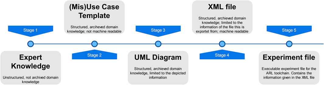
FIGURE 1. From expert knowledge to an experiment file for the ARL toolchain.

The first step of this process is knowledge gathering and, in stage 2, filling out the misuse case templates. These have to be very specific and well reviewed to be able to process the domain knowledge further. An error in this stage might lead to severe misunderstanding or wrong defined information and therefore wrong processes learned by the agent. This step is done by domain experts who are able to describe the domain knowledge in a sufficiently precise form. Since the MUC will be machine-read, enforcing certain syntactic elements is important (cf. Section 4 for details).

Afterwards, a STIX model of the misuse case scenario can be build for later usage.

The next step (stage 3) is the generation and annotation of an UML diagram that shows the relevant information to build an experiment file. MUCs will most likely contain at least one sequence diagram in any case. UML allows to introduce archetypes and parameters, building a model repository. We define custom stereotypes, like agent and environment, along with their parameters, which are then used to derive experiments definitions. Agents are of particular interest here, since our framework does not just employ DRL algorithms, but can use any agent. We define and implement simple agents with scripted behavior that reflects actors in the MUCs. These agents with hard-coded behavior are the experts that are necessary for imitation learning⁶.

The UML diagrams are exported to XMI; along with the MUC, they serve as a data source to derive experiment definitions (stage 4).

Stage 5 entails generating the experiment defintion file. We provide details about this file in Section 5. In general, an experiment file is the basis for a sound DoE, used for experimentation and training and evaluation of DRL agents. The experiments employ several agents in different experimentation phases. DRL agents can learn from the “scripted” agents. One methodology that commonly finds application in this setup is that of Adversarial Resilience Learning (ARL). In ARL, two (or possibly more) agents work as adversaries against each other. Agents do not have knowledge of each other or their respective actions, instead, they observe a system under influence by their adversary. This adversarial condition modifies the distribution of observed sensor inputs to encourage agents to sample more extreme regions, and also to learn more robust strategies. When two learning agents compete, they push each other to learn faster than an agent alone would normally do; learning agents working against a scripted agent also adapt counterstrategies faster in comparison to training solo. Sections 7 and 8 showcase such a competition setup.

After running the experiment, the STIX data can be updated with the found vulnerabilities as well as possible mitigation or attack differentiation.

4 Misuse case modelling and data transfer method

As mentioned in Section 2.2, the misuse-case method is used to precisely describe originally unintended behavior of a system. Therefore, all information from a mostyl regular IEC 62559-based use case template is included as well as the additional knowledge, which is distinctively used to document unintended behaviour.

The overall idea of this approach is to solve an existing semantic gap between two important aspects for the topic. In order to learn form proper attack libraries with real world incidents, a large amount of information for training is needed. Usually, in knowledge management, things are structures to refrain from being anecdotal. This leads to structures documents based on meta models making sure that all important aspects and attributes are covered and, thus, the information is self-contained and useful in a different context. This often involves eliciting the knowledge and experience of domain experts and stakeholders who are not experts in modeling. Structuring this knowledge into a standardized document leads to re-useable, useful knowledge. Often, this process is done in the context of systems engineering or development. However, it is apparent that the scope and detail as well as format for a learning AI is different. There is no fixed suitable API to re-use the use cases as of now. However, the large knowlwdge base both for use cases as well as misuse cases, documenting observable behaviour which is non-intended is large. Security incidents mostly are non-intended behaviour, so re-using the knowledge gathered in a structured manner is the aim discussed in detail in this contribution.

For this paper we do not consider misbehaviour of the system in terms of a faulty implementation but respective stakeholders, e.g, people acting maliciously. Therefore, the actors (and especially the misactors, called “crooks”) are in focus of the high-level modeling at first. Hence, these areas of the template must be filled out with particular care.

Two methods are conceivable for the proposed approach in this contribution: Use case supported elicitation of the templates and domain knowledge supported elicitation of the templates. In the first method, a completed use case template is examined to determine the undesired (system) behavior (or, in this case, the attacks) that could affect this use case. This can be done, e.g, by systematically checking the data within the MITRE ATT&CK data set identified to be suitable.

Algorithm 1. Pseudocode: Simplified Generation of a Experiment File from XML Data.

Open XML input file ⊳ MUC XML and/or diagram XML export

  name_list = empty list

  objective_list = empty list

  for actor in MUC do ⊳ either from UML actor definition or by scanning the actor tables in the MUC

   Add name of agent to name_list

   Add objective to objective_list

  end for

  Close XML input file

  Open YAML output file

 Write experiment setup data to the output file ⊳ This is simplified for a first presentation of this approach

 for agent_name in name_list do

  Write agent description to the output file ⊳ This data is a mixture of already created experiment definitions and the agent description from the input.

  Map agent objective from objective_list

  Write mapped objective to the output file

 end for⊳ The following is as well simplified for a first presentation of this approach

 Write sensor and actor information to the output file

 Define phases according to actor information in the output file

 Close YAML output file

 Output the generated YAML file

The second method is based on known attacks (in general terms: known undesired behavior) without an underlying use case in particular. Here, the misuse case template is filled in based on the known attack information and, thus, known mitigations.

By following one of these approaches, an domain expert is able to create a misuse case for the desired scenario. Afterwards, checking for consistency with other domain experts and by reviewing different modelling formats like the Smart Grid Architecture Model (SGAM) from the IEC SRD 63200 standard for the energy domain or the STIX data is recommended to rule out possible ambiguity and vagueness resulting from natural language usage.

For the approach presented in this paper, a nearly completed misuse case template is important as a base for the next steps since errors at this level are very likely to propagate to the next steps, thus, lowering the data quality and validity of the final conclusions to be drawn form the method.

After the MUC template is filled out, the diagrams and the tables of the MUC are exported as serialized and standardized XMI/XML files based on IEC 62559-3. Therefore, the diagrams are exported as a XMI from a tool like visual paradigm, while the MUC DOCX file is exported as a XML file via Microsoft Word. These files are then read into a script that generates an experiment file based on the information from the MUC and commonly known information such as the structure. The simplified version of this algorithm is presented as pseudocode in Algorithm 1. For the presentation of this approach only a limited set of information is taken from the MUC. The remaining needed information like, e.g. the environment and the mapped, distinct sensors in this environment are derived from a previous created experiment file.

For receiving the agent data the exported diagram is scanned for entities with the agent stereotype, if a MUC export is used to generate the experiment file, the XML is scanned for the actor table. From these sources the agent name and its objectives are taken. Afterwards the YAML output file is generated. Therefore the setup information from a already created experiment are taken (cf. Section 5 for a description of needed information). The information taken from the input is then merged with the additional information and put together to a complete experiment file.

5 Design of experiments with arsenAI

In order to tackle the problem outlined in Sections 1,2, namely, that currently, there exists no software stack that allows for sound, systematic, and reproducible experimentation of learning agents in CPSs (co-) simulation environments, we have created the palaestrAI software stack⁷. Part of the palaestrAI suite is a tool named arsenAI, whose focus is to read experiment definitions in YAML format. This experiment definition file contains environments, agents and their objective and defines parameters and factors to vary upon. An arsenAI run outputs a number of experiment run definitions, which contain concrete instantiations of the factors.

An experiment definition start with a unique, user-defined identifier (a unique name for the experiment), a seed value (for reproducibility), a version string to ensure software API compatibility, the number of repetitions and how many experiment runs should be generated from it. It also consists of a number of sub-definitions for agents, environments, sensor sets and actuator sets, and phase configurations.

An agent consists of a learner (nicknamed brain), an inference rollout worker (nicknamed muscle), as well as an objective. Objectives are agent-specific and based upon the reward definition of an environment, as well as the agent’s internal state. An environment has a reward definition: While the reward describes the states of the environment (e.g, bus voltages), the agent’s objective qualitatively describes the agent’s goal with regards to the current state/reward (e.g, the deviation from 1.0 pu).

Sensor and actuator sets connect environments to agents. A sensor is a particular input to an agent (e.g, a bus voltage), an actuator is a setpoint (e.g, reactive power generation).

An experiment is subdivided into phases, each phase describing a stage of the experiment. Therefore, an experiment also contains phase configuration definitions. A phase configuration describes whether agents learn (training mode) or only exploit their policy (testing mode), and how many episodes a phase consists of.

Within phases, factors are defined. Possible factors are the combination of agents, environments, phase configurations, and sensor/actuator-set-to-agent mappings. The environments and agents factors have two levels, since agents and environments can be combined.

After computing the design of the experiment, arsenAI decides on the sampling strategy. If the computed number of runs for a full factorial design from the factors (considering all levels) is less or equal than the user-defined maximum number of runs, a full factorial design is indeed generated. Otherwise, the full factorial design is optimized (i.e, sampled) according to the maximin metric (Pronzato and Walter, 1988).

Figure 2 shows a schema of the experiment definition.

FIGURE 2

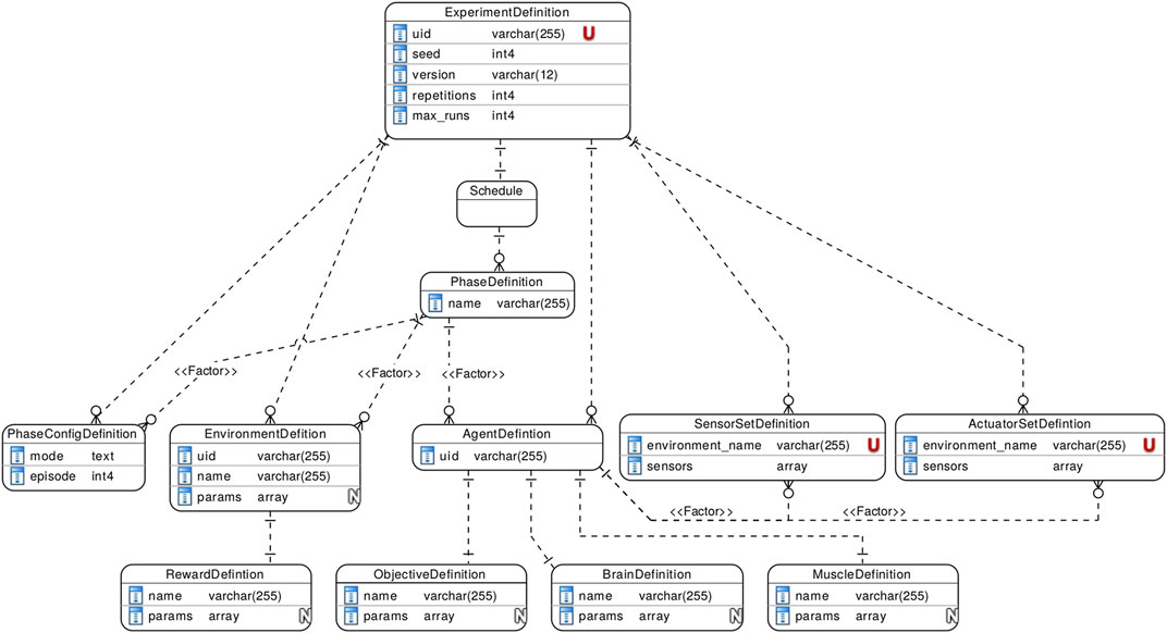
FIGURE 2. Experiment definition schema.

For each sample—and the number of desired repetitions—, arsenAI creates an experiment run definition, which is then picked up by palaestrAI to execute. We detail palaestrAI, along with agent designs and learning algorithms, in the next section, Section 6.

6 The palaestrAI execution framework

palaestrAI⁸ is the execution framework. It offers packages to implement or interface to agents, environments, and simulators. The main concern of palaestrAI is the orderly and reproducible execution of experiment runs, orchestrating the different parts of the experiment run, and storing results for later analysis.

palaestrAI’s Executor class acts as overseer for a series of experiment runs. Each experiment run is a definition in YAML format. Experiment run definitions are, in most cases, produced by running arsenAI on an experiment definition. An experiment defines parameters and factors; arsenAI them samples from a space filling design and outputs experiment run definitions, which are concrente instanciations of the experiment’s factors.

ExperimentRun objects represent such an experiment run definition as is executed. The class acts as a factory, instanciating agents along with their objectives, environments with corresponding rewards, and the simulator. For each experiment run, the Executor creates a RunGovernor, which is responsible for governing the run. It takes care of the different stages: For each phase, setup, execution, and shutdown or reset, and error handling.

The core design decision that was made for palaestrAI is to favor loose coupling of the parts in order to allow for any control flow. Most libraries⁹ enforce an OpenAI-Gym-style API, meaning that the agent controls the execution: The agent can reset() the environment, call step(actions) to advance execution, and only has to react to the step(⋅) method returning done. Complex simulations for CPSs are often realized as co-simulations, meaning that they couple domain specific simulators. Through co-simulation software packages like mosaik (Ofenloch et al., 2022), these simulators can exchange data; the co-simulation software synchronizes these simulators and takes care of proper time keeping. This, however, means that palaestrAI’s agents act just like another simulator from the perspective of the co-simulation software. The flow of execution is controlled by the co-simulator.

palaestrAI’s loose coupling is realized using ZeroMQ (Hintjens, 2023), which is a messaging system that allows for a reliable request-reply patterns, such as the majordomo pattern (Górski, 2022; Hintjens, 2023). palaestrAI starts a message broker (MajorDomoBroker) before executing any other command; the modules then either employ a majordomo client (sends a request and waits for the reply), or the corresponding worker (receives requests, executes a task, returns a reply). Clients and workers subscribe to topics, which are automatically created on first usage. This loose coupling through a messaging bus enables the co-simulation with any control flow.

In palaestrAI, the agent is split into a learner (Brain) and a rollout worker (Muscle). The muscle acts within the environment. It uses a worker, subscribed to the muscle’s identifier as topic name. During simulation, the muscle receives requests to act with the current state and reward information. Each muscle then first contacts the corresponding brain (acting as a client), supplying state and reward, requesting an update to its policy. Only then does the muscle infer actions, which constitute the reply to the request to act. In case of DRL brains, the algorithm trains when experiences are delivered by the muscle. As many algorithms simply train based on the size of a replay buffer or a batch of experiences, there is no need for the algorithm to control the simulation.

But even for more complex agent designs, this inverse control flow works perfectly fine. The reason stems directly from the MDP: Agents act in a state, s_t. Their action a_t triggers a transition to the state s_t+1. I. e, a trajectory is always given by a state, followed by an action, which then results in the follow-up state. Thus, it is the state that triggers the agent’s action; the state transition is the result of applying an agent’s action to the environment. A trajectory always starts with an initial state, not an initial action, i. e, τ = (s₀, a₀, …). Thus, the control flow as it is realized by palaestrAI is actually closer to the scientific formulation of DRL than the Gym-based control flow.

In palaestrAI, the SimulationController represents the control flow. It synchronizes data from the environment with setpoints from the agents, and different derived classes of the simulation controller implement data distribution/execution strategies (e.g, scatter-gather with all agents acting at once, or turn-taking, etc.)

Finally, palaestrAI provides results storage facilities. Currently, SQLite for smaller and PostgreSQL for larger simulation projects are supported, through SQLalchemy¹⁰. There is no need to provide a special interface, and agents, etc. do not need to take care of results storage. This is thanks to the messaging bus: Since all relevant data is shared via message passing (e.g, sensor readings, actions, rewards, objective values, etc.), the majordomo broker simply forwards a copy of each message to the results storage. This way, the database contains all relevant data, from the experiment run file through the traces of all phases to the “brain dumps,” i.e, the saved agent policies.

Figure 3 shows an excerpt of the palaestrAI software stack with the packages and classes mentioned until now.

FIGURE 3

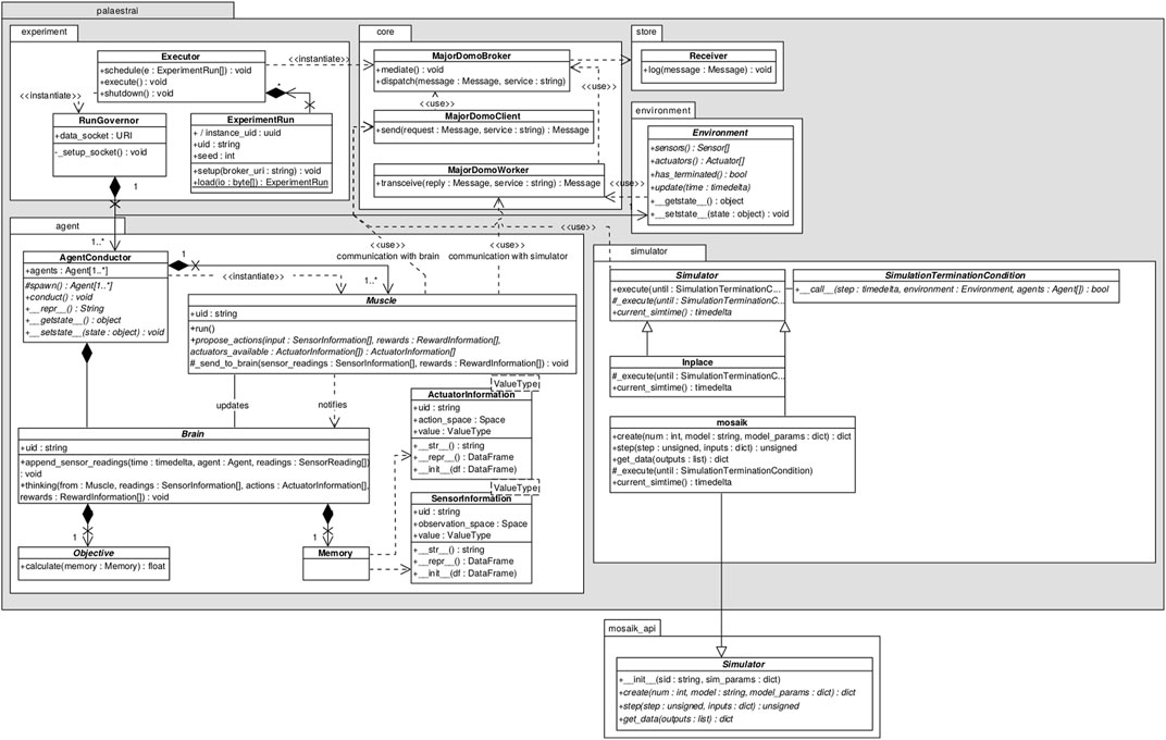
FIGURE 3. The palaestrAI core framework.

arsenAI’s and palaestrAI’s concept of experiment run phases allow for flexibility in offline learning or adversarial learning through autocurricula (Baker et al., 2020). Within a phase, agents can be employed in any combination and any sensor/actuator mapping. Moreover, agents—specifically, brains—can load “brain dumps” from other, compatible agents. This enables both offline learning and autocurricula within an experiment run in distinct phases.

7 Experimental concept validation

7.1 (Mis-) use cases considered

For initial validation of our approach, we describe two MUCs in the power grid domain that constitute clear attacks on normal grid operation. For both scenarios, we generate experiment definitions from the MUC; we execute the experiment runs and showcase the results in Section 8. We believe that this validates the initial feasibility of our approach. Since we focus on the software part of the approach, we do not provide extensive analysis of agents that have learned in an autocurriculum or offline learning scenario versus pure (single) DRL agent learning scenarios, as we regard this as future work.

The MUCs considered in this paper are.

• Inducing of artificial congestion as a fascailly motivated attack on local energy markets

• attacking reactive power controllers by learning oscillating behavior.

While the first MUC describes an internal misbehaviour in which the participating actors have the rights to control their components, while in the second MUC, the components controlled by the attacking agent have been corrupted.

7.1.1 Market exploitation misuse case

The first scenario, which is shown in Figure 4, can be described as a loophole in the operation of local energy markets. Local energy markets exist to allow operation of a (sub-) grid in a more efficient manner without needing grid expansion: They incentivize load shifting or feed-in adjustment to resolve congestion situation. Whenever the grid operator forecasts a congestion, it will place an offer on the local energy market for consumption reduction. Participants can bid on this offer, and if they adjust their consumption, they will receive compensation according to their bid.

FIGURE 4

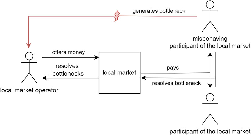
FIGURE 4. Misuse case actor diagram depicting energy market exploitation through artificially created congestions.

The loophole exists in market participants artificially creating the congestion. A group of participants can “game” the market by creating a bottleneck in their energy community (e.g., by charging electric vehicles). The grid operator will react by incentivizing load shifting. Since this load was created without a real need, it is easy for the crooks to place bids and, once won, follow the new load schedule in order to receive compensation. This can be repeated easily. The grid operator, however, is not able to distinguish this from legitimate demand, since consumers use the appliance they have access to in any normal case.

7.1.2 Voltage band violation attack through oscillating reactive power feed-in/consumption

The second considered scenario describes a different kind of attack. It is assumed that a attacker already claimed some components in the energy grid and is able to control them (e.g., photovoltaic panels). One of the main tasks in distribution grids is voltage control. DERs can be used for this through their inverters. Since the distribution grids have been carrying most of the DER installations, incorporating these into the voltage control scheme is an obvious strategy.

DERs also turn voltage control into a distributed task. We do not propose a new voltage control scheme; instead, we employ a distributed control scheme that has also been proposed and used by other authors. Namely, Zhu and Liu (2016) proposed a distributed voltage control scheme where the reactive power injection/consumption at a time t at each node is governed by:

$\mathit{q}\left(t+1\right)={\left[\mathit{q}\left(t\right)-\mathit{D}\left(\mathit{V}\left(t\right)-1\right)\right]}^{+},(1)$

where the notation [⋅]⁺ denotes a projection of invalid values to the range $[\underline{{\mathit{q}}^g},\overline{{\mathit{q}}^g}]$, i.e., to the feasible range of setpoints for q (t + 1) of each inverter. D is a diagonal matrix of step sizes.

We denote the attack strategy described by Ju and Lin (2018) as “hard-coded oscillating attacker behavior.” It can be described by a simple Mealy automaton with the internal state t, which is a time-step counter that represents the time the agent remains in a particular state. We note two states,

$Q=\left\{low,high\right\}.(2)$

This attacker remains in a particular state until a hold-off time T_h is reached. The hold-off time allows the benign voltage controller to adjust their reactive power feed-in/consumption, q(t). The attacker then suddenly inverts its own reactive power control, i. e, switches between $\underline{{\mathit{q}}^g}$ and $\overline{{\mathit{q}}^g}$.

$\delta \left(low,t\right)=\left\{\begin{array}{cc}high\hfill & \text{if\hspace{0.17em}}t=T_h,\hfill \\ low\hfill & \text{else,}\hfill \end{array}\right.(3)$

$\delta \left(high,t\right)=\left\{\begin{array}{cc}low\hfill & \text{if\hspace{0.17em}}t=T_h,\hfill \\ high\hfill & \text{else.}\hfill \end{array}\right.(4)$

Thus, $q(t,low)=\underline{{\mathit{q}}^g}$ and $q(t,high)=\overline{{\mathit{q}}^g}$.

In this scenario, the attacker wants to exploit the behavior (= AE) of the defending agent. Therefore, the attacking agent controls the assets taken over by him in a way that the voltage level is dropped or increased. In the next step the voltage band defending agent controls its assets to compensate the changes applied by the attacking agent. The attacking agent then operates contrary to his previous action. Therefore the compensation of the defender leads to an even higher outcome for the attacker.

In the next iteration the defending agent would again compensate by an even higher value also contrary to his previous action. The attacker would repeat his behaviour. These repeated behaviours then would lead into a pendulum movement of the voltage band and eventually lead to a loss of function as the deviation becomes to high to keep the energy grid stable.

For the simulation, we define the reward as a vectorized function of all bus voltage magnitudes observable by an agent, after all agent actions are applied:

${\mathit{r}}_{s,a}\left(t\right)={\left[V_1\left(t\right),V_2\left(t\right),\dots ,V_k\left(t\right),\dots ,V_n\left(t\right)\right]}^{\top },\forall V_k\left(t\right):V_k\left(t\right)=o\in \mathrm{\Omega }(5)$

As the agent’s objective expresses the desired state (i. e, goal) of the agent, we formulate p_Λ(r_s,a(t)) such that it induces an oscillating behavior, where the agent switches between full reactive power injection and full reactive power consumption within the boundaries of what the connected inverter is able to yield. Since we are not bound to formulate the objective in a specific way, we described this desired behavior by a function modeled after a normal distribution’s probability density function:

$g\left(x,A,\mu ,C,\sigma \right)=A\cdot \text{exp}\left(-\frac{{\left(x-\mu \right)}^2}{2{\sigma }^2}-C\right).(6)$

In order to encourage the agent to make use of the oscillating behavior, we formulate the attacker’s objective by using the reward machine device (Icarte et al., 2018). That is, we introduce three states, modeled as a Mealy state machine:

$Q=\left\{low,nominal,high\right\}.(7)$

The state machines alphabet Σ consists of the reward,

$\mathrm{\Sigma }=\left\{r_{s,a}^{\sim }=\mathrm{m}\mathrm{e}\mathrm{d}\mathrm{i}\mathrm{a}\mathrm{n}\left({\mathit{r}}_{s,a}\right)\forall {\mathit{r}}_{s,a}\right\}.(8)$

We transition between the three states based on the current reward as well as the time the reward machine’s initial state remains the same. This holdoff time T_h is chosen deliberately to give the benign voltage controllers time to adjust, i. e, to find equilibrium in the current extreme state the attacker agent has introduced. The state transition functions are thus.

$\delta \left(nominal,t\right)=\left\{\begin{array}{cc}low\hfill & \text{if\hspace{0.17em}}{r}_{s,a}^{\sim }\ge 1.05\wedge t=T_h,\hfill \\ high\hfill & \text{if\hspace{0.17em}}{r}_{s,a}^{\sim }\le 0.95\wedge t=T_h,\hfill \\ nominal\hfill & \text{else,}\hfill \end{array}\right.(9)$

$\delta \left(low,t\right)=\left\{\begin{array}{cc}nominal\hfill & \text{if\hspace{0.17em}}{r}_{s,a}^{\sim }\le 0.88\wedge t=T_h,\hfill \\ low\hfill & \text{else,}\hfill \end{array}\right.(10)$

$\delta \left(high,t\right)=\left\{\begin{array}{cc}nominal\hfill & \text{if\hspace{0.17em}}{r}_{s,a}^{\sim }\ge 1.12\wedge t=T_h,\hfill \\ high\hfill & \text{else.}\hfill \end{array}\right.(11)$

For each state, we define an objective function based on Eq. 6.

$p_{\mathrm{\Lambda },nominal}\left({\mathit{r}}_{s,a}\right)=g\left(r_{s,a}^{\sim },-\mathrm{12,1},-10,-0.05\right),(12)$

$p_{\mathrm{\Lambda },low}\left({\mathit{r}}_{s,a}\right)=g\left(r_{s,a}^{\sim },-\mathrm{14,0.84},-12,-0.08\right),(13)$

$p_{\mathrm{\Lambda },high}\left({\mathit{r}}_{s,a}\right)=g\left(r_{s,a}^{\sim },-\mathrm{14,1.16},-12,-0.08\right).(14)$

The values for A, μ, C, and σ are chosen by us deliberately to create the desired effect. Visual inspection of the resulting objective function, plotted over the voltage band in Figure 5, where the state transitions are marked by the vertical dashed lines, shows the desired shape that urges the agent to apply an oscillating behavior to foil simple reactive power controllers. Essentially, the attacker starts in the state fitting to the current reward $r_{s,a}^{\sim }$, which will most likely be q = nominal. As it then works towards over- or under-voltage. If attained, the agent remains in the state until the holdoff time is reached, all the while receiving positive objective value for keeping the extreme state. Note that the objective value will diminish due to the benign voltage controllers’ actions. Then, q ∈ {low, high} is chosen according to $r_{s,a}^{\sim }$. With the changed state, the agent receives a low objective value and is subsequently forced to act towards the other extreme voltage region. The state changes back to q = nominal, the agent’s momentum as well as the actions by the benign voltage controllers will yield the transition to the opposite extreme state. Note that δ(⋅) implements a hysteresis with regards to $r_{s,a}^{\sim }$.

FIGURE 5

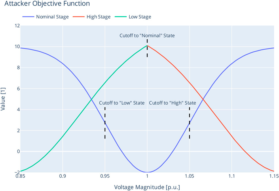
FIGURE 5. Attacker objective as a function of the voltage magnitude, with state transition boundaries.

7.2 Experiment setup

To validate the described method, an experimental setup was build. Therefore the needed information of the misuse cases described in chapter 7.1 were transferred to the misuse case template¹¹ described in Section 4. Afterwards this template (written in DOCX format) is exported to a XML-file. The next step is to then export the required information from this format and paste it into the YAML experiment description presented in chapter 5. The considered information in the experimental setup is the objective as well as the name of the agents. To achieve the correct syntax, the agents entered objectives are mapped to the syntax of the file in YAML format. In this experimental setup, the exact input is used. Therefore, a strict restriction is given.

For our experiment, we additionally employ the MIDAS¹² software suite that provides the simulation environment setup: It incorporates the PySimMods¹³ software package that contains numerous models for power grid units, such as batteries, Photovoltaic (PV) or Combined Heat and Power (CHP) power plants. The grid model is a CIGRÉ Medium Voltage (MV) grid model (Rudion et al., 2006).

Each node has a constant load of 342 + j320 kVA attached to; the loads are not subject to time series, but remain constant in all experiment scenarios. This constant load accounts for the real power feed-in that occurs naturally because of the inverter model. The goal is to maintain an average voltage magnitude close to 1.0 pu on every bus if no action is taken. This way, the reactive power controllers suffer no handicap in their ability to feed or consume reactive power when the attack starts. The power grid has 9 PV power plants attached at buses 3 to 9, 11, and 13. The PV plants’ output is dependent on the solar irridation, which is governed by a multi-year weather dataset from Bremen, Germany¹⁴. The PV installations vary between P_peak = 8.2 kW to 16.9 kW, with cos φ = 0.9. This represents smaller PV plants in rural areas as a realistic setup. The individual values in this range have been chosen so that the reactive power control scheme can maintain 1.0 pu on all relevant buses without using the full capability range of the inverters. We have deliberately chosen not to include any consumers governed by load profiles in order to make the effect of the controlled inverters visible in isolation; we rely on the aforementioned constant load to provide a balanced grid without tap changers or other measures.

The attacker controls the buses 3, 4, and 8, as depicted in Figure 6. Buses 5, 7, 9, and 11 are governed by the distributed voltage control scheme. To each attacker and defender bus, a PV plant is connected. The other buses are not governed by any controller. Each benign voltage controller applies the distributed control law (Zhu and Liu, 2016) as described in Eq. 1. We have chosen D = 10J for all experiments as this provides stable operation in all normal cases and allows the voltage controllers to converge at 1.0 pu quickly.

FIGURE 6

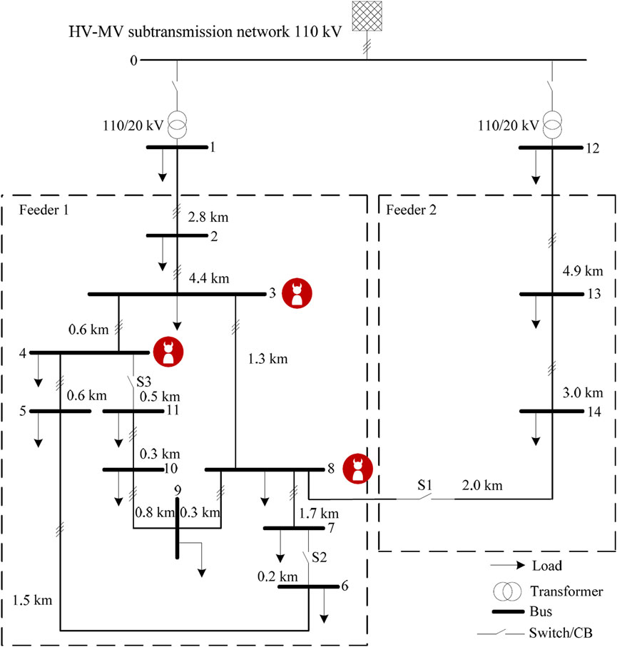
FIGURE 6. The CIGRÉ MV grid used for the simulation, with attacker nodes marked.

8 Initial results

After completing the MUC templates, a STIX 2.1 file was created for both scenarios. The STIX visualization for the local market MUC and the oscillating attack MUC is shown in Figures 7, 8, respectively.

FIGURE 7

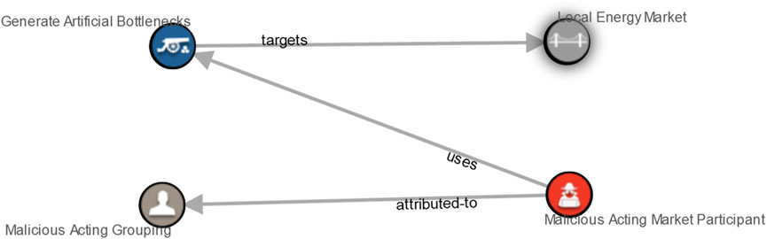
FIGURE 7. STIX visualization of the energy market exploitation through artificial congestion misuse case.

FIGURE 8

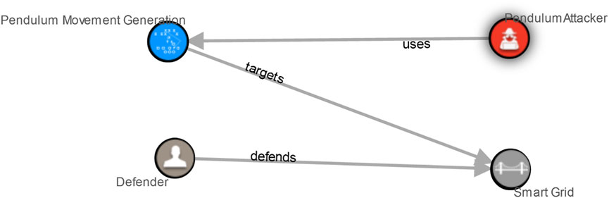
FIGURE 8. STIX visualization of the voltage band violation attack misuse case.

From the oscillation MUC, we have derived 10 distinct simulation phases: Two baseline phases, in which only the voltage controller acted (with and without time series). Then, two reproduction phases implementing the voltage controller and the “hard-coded” oscillating attacker. Three phases then pitched learning agents as attackers against the voltage controller without time series for solar irradiation (using DDPG, PPO, and TD3). Finally, three phases with learning agents against the voltage controller with time series for PV feed-in (again, using DDPG, PPO, and TD3). For a more concise naming, we attribute all phases without time series as “static” and those with time series data as “dynamic.”

Figure 9 shows a box plot of the voltage magnitudes at the victim buses for each phase. The boxplot is based on the raw data available in Table 1. Additionally, Table 2 counts the voltage band violations for each phase.

FIGURE 9

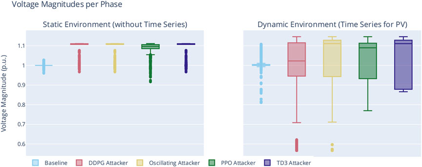
FIGURE 9. Voltage magnitudes for each experiment phase in the voltage band violation scenario.

TABLE 1

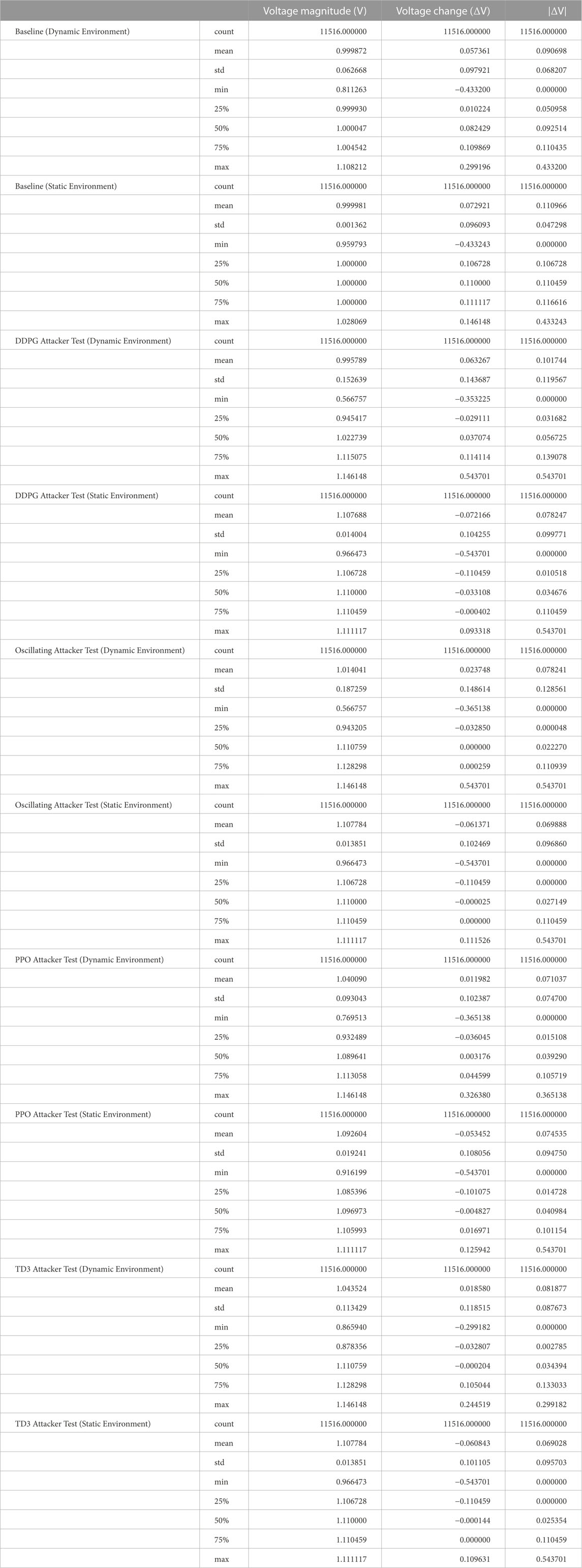
TABLE 1. Bus voltage statistics per phase.

TABLE 2

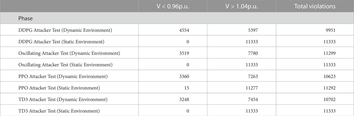
TABLE 2. Number of voltage band violations.

The baseline phases verify that the reactive power controller works, because apart from some outliers that are due to initial swing-in behavior of the controller (cf. also the baseline in Figure 10), voltage median is at 1.0 pu.

FIGURE 10

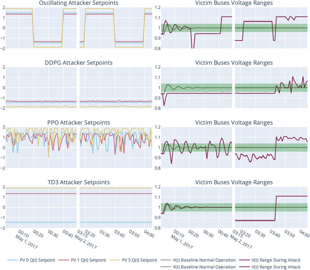
FIGURE 10. Setpoints of the attackers’ actuators as well as the obtained objective value. Note that the graphs contain an intentional time gap between 00:50 and 03:15.

All “attacker” boxes in Figure 9 show deviation from 1.0 pu. The hard-coded oscillating attacker sets the Voltage Magnitude (VM) median value to ≈1.1 pu in the “static” as well as in the “dynamic” environment phase. From this, we infer that the attack was indeed effective. The maximum VM in terms of voltage is 1.11 pu for the static, and 1.146 pu in the dynamic case. As the only difference between the two phases the introduction of time series, we believe that, in general, the hard-coded oscillating behavior amplifies the effect of change in solar irradiation over the day. However, due to the hard-coded nature of the simple attacker, finding the “right” moment to leverage, e. g, sunrise happens most probably by coincidence, since T_h is static.

The Oscillating Attacker phases in Figures 9, 10 serve as an additional baseline in order to reproduce and ascertain the attack documented by Ju and Lin (2018). As the effects of this kind of attack have already been published, these phases serve as a validation of our simulation set-up and baseline for comparison. Thus, we believe that the effectiveness of the original attack has been reproduced, and the relationship (Ju and Lin, 2018) holds:

$\underset{T_h\to \infty }{\lim }\left[{\mathit{V}}_b\left(T_h+1\right)\right]=-2\left[\mathit{X}\right]\bar{\mathit{q}},(15)$

where T_h is the hold-off time of the attacker (usually until the victim buses have reached equilibrium), X is the reactance of the subgrid with the attackers as root nodes, and $\bar{\mathit{q}}$ represents the extreme reactive power value of the attacker (either feed-in or consumption).

Through Figure 9, we can compare these baselines to the phases in which the learning agents are employed. All algorithms also obtain a maximum VM of 1.1 pu and 1.146 pu (static and dynamic environment, respectively), which seems to be the maximum attainable VM for our simulation setup. Considering the VM ranges obtained by the learning agents, the high medium VM, which are on par with the hard-coded oscillating attacker (with the exception of DDPG in the dynamic environment), the simulation results indicate that the learning agents have discovered an attack.

As scenario 2 enables time series for solar irradiation, we observe that good timing of the oscillation increases the deviating effect on the voltage band, most probably owing to the real-power feed-in happens in addition to the effect of the reactive power curve on voltage levels.

Scenarios 3 and 4 replace the simple oscillating attacker with an DRL-based agent. The phases are, in accordance, labeled from the algorithm that was employed: DDPG, PPO, or TD3. Again, Figure 9 establishes that each agent was able to generate an effect that can be seen as an attack to the power grid. Each produced the same maximum voltage level, with DDPG obtaining the exact same under-voltage level and in general similar values—albeit with a lower median, close to 1.0 pu—as the simple oscillating attacker. Notably, PPO- and TD3-based attackers did not produce any outliers while maintaining a high median in the dynamic environment. The box plot of the TD3-based attacker suggests that this is the deadliest attacker, obtaining a high voltage band deviation (median VM, no outliers) throughout the simulation runs.

In order to verify our imitation learning hypothesis, we must establish whether the agents have actually learned to attack. The most commonly used method to infer whether an agent has learned to reach a certain objective is to analyze its objective function, which is the agent-specific reward for a state transition, considering its goal. We have already described the employed attacker objective in Eq. 12. Figure 11 plots the objective function (raw objective as well as moving average) for all four attacker phases for the “dynamic” grid, i. e, with time series for solar irradiation.

FIGURE 11

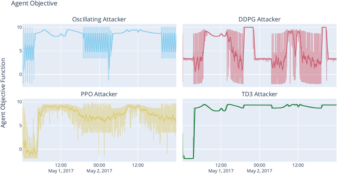
FIGURE 11. Attacker objective function, plotted over simulation time. Light colors depict absolute values, bold lines the moving avarage with a window of 100∼steps.

The objective plot of the simple oscillating attacker is straightforward, showing the oscillation clearly during the night, when the PV inverters’ capabilities directly influence the grid. During the day, the real power feed-in leads to over-voltage, no longer making the oscillating behavior effective or even visible.

DRL essentially solves the optimization problem, that each algorithm ultimately attempts to find an optimal policy π* by maximizing the agent’s objective function. We can therefore infer the attacker agents’ policy from the objective function plots.

Both the DDPG-based as well as the PPO-based agent have derived a policy that incorporates an oscillating behavior. Although the DDPG-based agent was not able to yield behavior that came close to the original attack, with only mediocre average objective values.

The PPO-trained agent, on the other hand, obtained higher average objective values while still showing the oscillating behavior of the original attack. It obtained reliable over- and undervoltages. From the shape of the objective function (cf. Figure 5), we know that residing in extreme values is discouraged by the objective (and values close to 1.0 pu are penalized). PPO takes advantage of daytime solar irradiation but maintains the oscillating behavior even during midday.

TD3 shows to be the most interesting of all attackers. The TD3-based attacker has learned no oscillating behavior at all. However, the policy obtained by training with TD3 manages to yield consistently high objective values. By simple deduction, we can therefore infer that the oscillating behavior of malicious inverters is not necessary to yield appropriate damage to victim buses.

Investigating actual agent behavior during two timeframes in Figure 10 in combination with data displayed in Figures 9, 11 gives rise to the hypothesis that (1) damaging the power grid does not need oscillating behavior, (2) can have an equally high impact, and (3) is potentially more dangerous as it does need several oscillating steps, thus making it more surprising for benign buses and the grid operator. None of the learning agents possessed any domain knowledge or had access to sensors apart from its own, node-local ones. While the TD3-based agent has simply learned a vector of setpoints that will eventually prove to be fatal, the DDPG-based attacker’s slight oscillations cause the benign reactive power controller to yield stark oscillating behavior, too.

9 Discussion

Our approach creates a bridge between informal modelling of domain expert knowledge in terms of scenarios to rigorous experimentation with learning agents. The second MUC—the one that shows the oscillation attack—is a simple, yet comprehensive scenario that allows to verify the general hypothesis, that MUCs can be part of a immediate pipeline allowing to train agents in an offline learning or autocurriculum.

Our initial approach outlined in this article uses an expert through the objective as a simple form of imitation learning, specifically, behavior cloning. The objective we presented in the experimental validation is a very focused one, based on the behavior we model in the MUC. It is based on an already known behavior, specifically created to teach the agent an exact strategy. However, the DRL agents have discovered another behavior that led to the same goal, but exhibited a different behavior, even though the objective was not changed between phases. While PPO immitated the original strategy quite well, did TD3 resort to fixed setpoints that maximized reward without oscillating. Considering a “following the goal by intention,” this makes the TD3-based agent the potentially most destructive one, as it avoids steep gradients, which would quickly alert the grid operator, because they violate grid codes. Therefore, we assume that using the agent’s objective as expert for behavior cloning is not only effective, but also does not hinder the agent in devision new attack vectors when it has the chance to interact with the environment.

Nevertheless, it is not known whether an agent would have learned a different strategy to achieve the goal without the specified behavior. Therefore, running additional experiments without predefined trajectories might be beneficial in cases where a general approach without specified behaviour is wanted. Regardless of this, the approach presented here can still be useful in such a situation because general concepts can be passed as trajectories that do not describe a direct, goal-directed action. An example is bidding on a local market, which does not yet describe misbehavior, but conveys the basic concepts for dealing with the market to the agent.

The most cumbersome part of our approach is the fact that the domain expert still needs a MUC modelling expert familiar with our approach to apply the correct stereotypes and to ensure that the correct XML/XMI file is created. Otherwise, depending on the severity of the syntax and semantic errors, our approach might lead to wrong learned behaviour or not executable experiments. Still, this technical breakthrough allows extension now that baseline scenarios have been established. For example, a direction of research could employ text recognition in the way ChatGPT was trained to arrive at properly formatted MUCs from non-precise wording.

10 Conclusion and future work

In this article, we have demonstrated a software framework that enables sound experimentation from MUC descriptions and embedded diagrams. Our approach enables domain experts to model scenarios, which are then analyzed by using learning agents. Moreover, our approach enables autocurricula and a limited form of offline learning by imitation learning with experts through the agents’ objectives. We have furthermore shown two MUCs, which have been converted into experiment definitions; one scenario has been extensively simulated and analyzed.

For future work, we will construct trajectories from sequence diagrams, extending the offline learning approach significantly. It might also be interesting to examine whether agents learn different strategies in the same environment when provided with knowledge through this approach, or whether, given sufficient training time, both procedures lead to the same behavior. As such, we plan to extend the MIDAS benchmark environment further, adding more domains, such as ICT. We will then build a repository of MUCs, and likewise, agents trained on there MUCs.

We expect to open the domain of online learning, or, more specifically, lifelong learning at this point. Agents can learn from multiple MUCs (not just one MUC per agent). However, this will surely lead the agents to encounter the plasticity-stability dilemma, where agents need to retrain learned behavior while learning new tasks. We will verify and analyze this, and propose a more complex agent that is able to incorporate knowledge from multiple MUCs.

Data availability statement

The datasets presented in this study can be found in online repositories. The names of the repository/repositories and accession number(s) can be found below: https://gitlab.com/arl-experiments.

Author contributions

EV contributed the introduction, sections on DRL, the descriptions of arsenAI and palaestrAI, as well as the execution and analysis of the oscillating voltage attack. AW contributed sections on the MUCs and the converter for MUC/XML to arsenAI experiment file. MU transferred the MUC methodology to power grid scenarios in general. He co-designed the MUCs for the scenarios described in this article.

Funding

This work has been funded by the German Federal Ministry for Education and Research (Bundesministerium für Bildung und Forschung, BMBF) under the project grant Adversarial Resilience Learning (01IS22071). The work on the Misuse Case Methodology has been funded by the German Federal Ministry for Economic Affairs and Climate Action (Bundesministerium für Wirtschaft und Klimaschutz, BMWK) under the project grant RESili8 (03EI4051A).

Conflict of interest

The authors declare that the research was conducted in the absence of any commercial or financial relationships that could be construed as a potential conflict of interest.

Publisher’s note

All claims expressed in this article are solely those of the authors and do not necessarily represent those of their affiliated organizations, or those of the publisher, the editors and the reviewers. Any product that may be evaluated in this article, or claim that may be made by its manufacturer, is not guaranteed or endorsed by the publisher.

Footnotes

¹This template is not the same as the template from the IEC 62559-2 standard.

²For a detailed view on the MUC template see: https://gitlab.com/arl2/muclearner.

³The tutorial by Levine et al. (2020) is available only as preprint. However, to our knowledge, it constitutes one of the best introductionary seminal works so far. Since it is a tutorial/survey, and not original research, we cite it despite its nature as a preprint and present it alongside the peer-reviewed publication by Prudencio et al. (2022), which cites the former, too.

⁴https://github.com/Farama-Foundation/Gymnasium, retrieved: 2022-01-03.

⁵The technical report for Horizon is available only as preprint. We treat it the same way as a website reference and provide the bibliography entry here for easier reference.

⁶At a later stage, we also plan to directly derive trajectories by parsing sequence diagrams, but this is currently future work.

⁷https://gitlab.com/arl2, retrieved: 2023-01-03.

⁸https://gitlab.com/arl2/palaestrai, retrieved: 2023-01-03.

⁹cf. Section 2.

¹⁰https://www.sqlalchemy.org/, retrieved: 2023-01-04.

¹¹These templates can be found here: https://gitlab.com/arl2/muclearner.

¹²https://gitlab.com/midas-mosaik/midas, retrieved: 2023-01-04.

¹³https://gitlab.com/midas-mosaik/pysimmods, retrieved: 2023-01-04.

¹⁴Publicly available from https://opendata.dwd.de/climate_environment/CDC/observations_germany/climate_urban/hourly/, last accessed on 2022-12-21.

References

Adawadkar, A. M. K., and Kulkarni, N. (2022). Cyber-security and reinforcement learning — a brief survey. Cyber-security Reinf. Learn. — a brief Surv. 114, 105116. doi:10.1016/j.engappai.2022.105116

CrossRef Full Text | Google Scholar

Apoorva, M., Eswarawaka, R., and Reddy, P. V. B. (2017). “A latest comprehensive study on structured threat information expression (STIX) and trusted automated exchange of indicator information (TAXII),” in Proceedings of the 5th International Conference on Frontiers in Intelligent Computing: Theory and Applications. Advances in intelligent systems and computing. Editors S. C. Satapathy, V. Bhateja, S. K. Udgata, and P. K. Pattnaik, 477–482. doi:10.1007/978-981-10-3156-4_49

CrossRef Full Text | Google Scholar

Baker, B., Kanitscheider, I., Markov, T., Wu, Y., Powell, G., McGrew, B., et al. (2020). “Emergent tool use from multi-agent autocurricula,” in International Conference on Learning Representations.

Google Scholar

Barnum, S. (2012). Standardizing cyber threat intelligence information with the structured threat information expression (STIX). Mitre Corp. 11, 1–22.

Google Scholar

Berghout, T., Benbouzid, M., and Muyeen, S. M. (2022). Machine learning for cybersecurity in smart grids: A comprehensive review-based study on methods, solutions, and prospects. prospects 38, 100547. doi:10.1016/j.ijcip.2022.100547

CrossRef Full Text | Google Scholar

Briliyant, O. C., Tirsa, N. P., and Hasditama, M. A. (2021). “Towards an automated dissemination process of cyber threat intelligence data using STIX,” in 2021 6th International Workshop on Big Data and Information Security (IWBIS), 109–114. doi:10.1109/IWBIS53353.2021.9631850

CrossRef Full Text | Google Scholar

Brockman, G., Cheung, V., Pettersson, L., Schneider, J., Schulman, J., Tang, J., et al. (2016). Openai gym.

Google Scholar

Bush, S. F. (2014). Smart grid: Communication-enabled intelligence for the electric power grid. IEEE. Chichester, UL: John Wiley & Sons.

Google Scholar

Castro, P. S., Moitra, S., Gelada, C., Kumar, S., and Bellemare, M. G. (2018). Dopamine: A research framework for deep reinforcement learning.

Google Scholar

Clausen, M., Apel, R., Dorchain, M., Postina, M., and Uslar, M. (2018). Use case methodology: A progress report. Energy Inf. 1, 19–283. doi:10.1186/s42162-018-0036-0

CrossRef Full Text | Google Scholar

Cockburn, A. (2001). Writing effective use cases. London, UK: Pearson Education).

Google Scholar

Connolly, J., Davidson, M., and Schmidt, C. (2014). The trusted automated exchange of indicator information (TAXII) (The MITRE Corporation), 1–20.

Fischer, L., Memmen, J. M., Veith, E. M., and Tröschel, M. (2019). “Adversarial resilience learning—Towards systemic vulnerability analysis for large and complex systems,” in ENERGY 2019, The Ninth International Conference on Smart Grids, Green Communications and IT Energy-aware Technologies (IARIA XPS Press), 24–32.

Google Scholar

Frost, E., Veith, E. M., and Fischer, L. (2020). “Robust and deterministic scheduling of power grid actors,” in 7th International Conference on Control, Decision and Information Technologies (CoDIT) (IEEE), 1–6.

CrossRef Full Text | Google Scholar

Fujimoto, S., Hoof, H., and Meger, D. (2018). “Addressing function approximation error in actor-critic methods,” in Proceedings of the 35th International Conference on Machine Learning (PMLR), 1587–1596 (Stockholm, Sweden: ISSN), 2640–3498.

Google Scholar

Gauci, J., Conti, E., Liang, Y., Virochsiri, K., Chen, Z., He, Y., et al. (2018). Horizon: Facebook’s open source applied reinforcement learning platform. arXiv preprint arXiv:1811.00260.

Google Scholar

Górski, T. (2022). Uml profile for messaging patterns in service-oriented architecture, microservices, and internet of things. Appl. Sci. 12, 12790. doi:10.3390/app122412790

CrossRef Full Text | Google Scholar

Gottschalk, M., Uslar, M., and Delfs, C. (2017). The use case and smart grid architecture model approach: The IEC 62559-2 use case template and the SGAM applied in various domains. Springer.

Google Scholar

Haarnoja, T., Zhou, A., Abbeel, P., and Levine, S. (2018). Soft actor-critic: Off-policy maximum entropy deep reinforcement learning with a stochastic actor.

Google Scholar

Hessel, M., Modayil, J., Van Hasselt, H., Schaul, T., Ostrovski, G., Dabney, W., et al. (2018). “Rainbow: Combining improvements in DQN,” in The Thirty-Second AAAI Conference on Artificial Intelligence (AAAI-18), 3215–3222.

Google Scholar

Hintjens, P. (2023). 0MQ — the guide, 4. Sebastopol, CA: O'Reilly.

Google Scholar

Holly, S., Nieße, A., Tröschel, M., Hammer, L., Franzius, C., Dmitriyev, V., et al. (2020). Flexibility management and provision of balancing services with battery-electric automated guided vehicles in the Hamburg container terminal Altenwerder (SpringerOpen). Energy Inf.

Google Scholar

Hong, J., Liu, C.-C., and Govindarasu, M. (2014). “Detection of cyber intrusions using network-based multicast messages for substation automation,” in Isgt 2014, 1–5. doi:10.1109/ISGT.2014.6816375

CrossRef Full Text | Google Scholar

Hu, L., Wang, Z., Han, Q.-L., and Liu, X. (2018). State estimation under false data injection attacks: Security analysis and system protection. Automatica 87, 176–183. doi:10.1016/j.automatica.2017.09.028

CrossRef Full Text | Google Scholar

Huang, B., Cardenas, A. A., and Baldick, R. (2019). “Not everything is dark and gloomy: Power grid protections against IoT demand attacks,” in Procedings of the 28th USENIX Security Symposium, Santa Clara, CA, USA (Berkeley, CA: Usenix Association).

Google Scholar

Icarte, R. T., Klassen, T., Valenzano, R., and McIlraith, S. (2018). “Using reward machines for high-level task specification and decomposition in reinforcement learning,” in Proceedings of the 35th International Conference on Machine Learning (Stockholm, Sweden: PMLR), 2107–2116.

Google Scholar

IEA (2019). Status of power system transformation 2019. Paris, France: resreport, IEA. CC-BY-SA 4.0.

Google Scholar

Inayat, U., Zia, M. F., Mahmood, S., Berghout, T., and Benbouzid, M. (2022). Cybersecurity enhancement of smart grid: Attacks, methods, and prospects. Attacks, methods, prospects 11, 3854. doi:10.3390/electronics11233854

CrossRef Full Text | Google Scholar

Ju, P., and Lin, X. (2018). “Adversarial attacks to distributed voltage control in power distribution networks with DERs,” in Proceedings of the Ninth International Conference on Future Energy Systems, 291–302. doi:10.1145/3208903.3208912

CrossRef Full Text | Google Scholar

Kuhnle, A., Schaarschmidt, M., and Fricke, K. (2017). Tensorforce: A tensorflow library for applied reinforcement learning.

Google Scholar

Levine, S., Kumar, A., Tucker, G., and Fu, J. (2020). Offline reinforcement learning: Tutorial, review, and perspectives on open problems. arXiv. doi:10.48550/arXiv.2005.01643

CrossRef Full Text | Google Scholar

Liang, E., Liaw, R., Nishihara, R., Moritz, P., Fox, R., Goldberg, K., et al. (2018). “RLlib: Abstractions for distributed reinforcement learning,” in International Conference on Machine Learning (ICML).

Google Scholar

Lillicrap, T. P., Hunt, J. J., Pritzel, A., Heess, N., Erez, T., Tassa, Y., et al. (2016). “Continuous control with deep reinforcement learning,” in 4th International Conference on Learning Representations, ICLR 2016 - Conference Track Proceedings.

Google Scholar

Liu, Y., Ning, P., and Reiter, M. K. (2011). False data injection attacks against state estimation in electric power grids. ACM Trans. Inf. Syst. Secur. (TISSEC) 14, 1–33. doi:10.1145/1952982.1952995

CrossRef Full Text | Google Scholar

Mahela, O. P., Khosravy, M., Gupta, N., Khan, B., Alhelou, H. H., Mahla, R., et al. (2022). Comprehensive overview of multi-agent systems for controlling smart grids. CSEE J. Power Energy Syst. 8, 115–131. doi:10.17775/CSEEJPES.2020.03390

CrossRef Full Text | Google Scholar

Mathas, C.-M., Vassilakis, C., Kolokotronis, N., Zarakovitis, C. C., and Kourtis, M.-A. (2021). On the design of IoT security: Analysis of software vulnerabilities for smart grids. MDPI Energies 14, 2818. doi:10.3390/en14102818

CrossRef Full Text | Google Scholar

Mnih, V., Kavukcuoglu, K., Silver, D., Graves, A., Antonoglou, I., Wierstra, D., et al. (2013). Playing atari with deep reinforcement learning. arXiv preprint arXiv:1312.5602.

Google Scholar

Nair, A. S., Hossen, T., Campion, M., Selvaraj, D. F., Goveas, N., Kaabouch, N., et al. (2018). Multi-agent systems for resource allocation and scheduling in a smart grid. Technol. Econ. Smart Grids Sustain. Energy 3, 15. doi:10.1007/s40866-018-0052-y

CrossRef Full Text | Google Scholar

Neureiter, C., Engel, D., Trefke, J., Santodomingo, R., Rohjans, S., and Uslar, M. (2014). “Towards consistent smart grid architecture tool support: From use cases to visualization,” in IEEE PES Innovative Smart Grid Technologies, Europe (IEEE), 1–6.

CrossRef Full Text | Google Scholar

OASIS Open Cyber Threat Intelligence Committee (2022). Introduction to STIX. Availableat: https://oasis-open.github.io/cti-documentation/stix/intro (Accessed 02 2023, 01).

Google Scholar

Ofenloch, A., Schwarz, J. S., Tolk, D., Brandt, T., Eilers, R., Ramirez, R., et al. (2022). “Mosaik 3.0: Combining time-stepped and discrete event simulation,” in 2022 Open Source Modelling and Simulation of Energy Systems (Piscataway, NJ: OSMSES), 1–5. doi:10.1109/OSMSES54027.2022.9769116

CrossRef Full Text | Google Scholar

OMG Group (2005). Xmi^TM: Xml metadata interchange. web page.

Google Scholar

Peng, X. B., Kumar, A., Zhang, G., and Levine, S. (2019). Advantage-weighted regression: Simple and scalable off-policy reinforcement learning. arXiv. doi:10.48550/arXiv.1910.00177

CrossRef Full Text | Google Scholar

Pronzato, L., and Walter, E. (1988). Robust experiment design via maximin optimization. Math. Biosci. 89, 161–176. doi:10.1016/0025-5564(88)90097-1

CrossRef Full Text | Google Scholar

Prudencio, R. F., Maximo, M. R. O. A., and Colombini, E. L. (2022). A survey on offline reinforcement learning: Taxonomy, review, and open problems. arXiv. doi:10.48550/arXiv.2203.01387

CrossRef Full Text | Google Scholar

Raffin, A., Hill, A., Gleave, A., Kanervisto, A., Ernestus, M., and Dormann, N. (2021). Stable-baselines3: Reliable reinforcement learning implementations. J. Mach. Learn. Res. 22, 1–8.

Google Scholar

Roberts, C., Ngo, S.-T., Milesi, A., Peisert, S., Arnold, D., Saha, S., et al. (2020). “Deep reinforcement learning for DER cyber-attack mitigation,” in 2020 IEEE International Conference on Communications, Control, and Computing Technologies for Smart Grids (Piscataway, NJ: SmartGridComm), 1–7. doi:10.1109/SmartGridComm47815.2020.9302997

CrossRef Full Text | Google Scholar

Roberts, C., Ngo, S.-T., Milesi, A., Scaglione, A., Peisert, S., and Arnold, D. (2021). “Deep reinforcement learning for mitigating cyber-physical der voltage unbalance attacks,” in 2021 American Control Conference (ACC), 2861–2867. doi:10.23919/ACC50511.2021.9482815

CrossRef Full Text | Google Scholar

Roche, R., Lauri, F., Blunier, B., Miraoui, A., and Koukam, A. (2013). Multi-agent technology for power system control. J. Abbr. Green Energy Technol. 59, 567–609. doi:10.1007/978-1-4471-5104-3_15

CrossRef Full Text | Google Scholar

Rudion, K., Orths, A., Styczynski, Z., and Strunz, K. (2006). “Design of benchmark of medium voltage distribution network for investigation of dg integration,” in 2006 IEEE Power Engineering Society General Meeting, 6–14. doi:10.1109/PES.2006.1709447

CrossRef Full Text | Google Scholar

Santodomingo, R., Uslar, M., Göring, A., Gottschalk, M., Nordström, L., Saleem, A., et al. (2014). “SGAM-based methodology to analyse smart grid solutions in discern European research project,” in 2014 IEEE International Energy Conference (ENERGYCON IEEE), 751–758.

CrossRef Full Text | Google Scholar

Schrittwieser, J., Antonoglou, I., Hubert, T., Simonyan, K., Sifre, L., Schmitt, S., et al. (2019). Mastering Atari, Go, chess and shogi by planning with a learned model. Nature 588, 604–609. doi:10.1038/s41586-020-03051-4

CrossRef Full Text | Google Scholar

Schulman, J., Wolski, F., Dhariwal, P., Radford, A., and Klimov, O. (2017). Proximal policy optimization algorithms. doi:10.48550/arXiv.1707.06347

CrossRef Full Text | Google Scholar

Schütz, J., Clausen, M., Uslar, M., and Gómez, J. M. (2021). “IEC 62559-2 use case template-based smart grid architecture analytics,” in CIRED 2021-The 26th International Conference and Exhibition on Electricity Distribution (IET), 2935–2939.

Google Scholar

Seno, T., and Imai, M. (2022). d3rlpy: An offline deep reinforcement learning library. J. Mach. Learn. Res. 23, 1–20.

Google Scholar

Silver, D., Huang, A., Maddison, C. J., Guez, A., Sifre, L., Van Den Driessche, G., et al. (2016a). Mastering the game of Go with deep neural networks and tree search. Nature 529, 484–489. doi:10.1038/nature16961

PubMed Abstract | CrossRef Full Text | Google Scholar

Silver, D., Hubert, T., Schrittwieser, J., Antonoglou, I., Lai, M., Guez, A., et al. (2017). A general reinforcement learning algorithm that masters chess, shogi, and Go through self-play. Science 362, 1140–1144. doi:10.1126/science.aar6404

CrossRef Full Text | Google Scholar

Silver, D., Schrittwieser, J., Simonyan, K., Nature, I. A., Huang, A., Guez, A., et al. (2016b). Mastering the game of Go without human knowledge. Nature 550, 354–359. doi:10.1038/nature24270

CrossRef Full Text | Google Scholar

Sindre, G., and Opdahl, A. L. (2005). Eliciting security requirements with misuse cases. Requir. Eng. 10, 34–44. doi:10.1007/s00766-004-0194-4

CrossRef Full Text | Google Scholar

Sindre, G., and Opdahl, A. L. (2001). “Templates for misuse case description,” in Proceedings of the 7th International Workshop on Requirements Engineering, Switzerland (Foundation for Software Quality (REFSQ’2001).

Google Scholar

Soltan, S., Mittal, P., and Poor, V. H. (2018). “BlackIoT: IoT botnet of high wattage devices can disrupt the power grid | USENIX,” in Proceedings of the 28th Usenix Security Symposium, Baltimore, MA, USA (Berkeley, CA: Usenix Association).

Google Scholar

Styczynski, J., and Beach-Westmoreland, N. (2016). When the lights went out: Ukraine cybersecurity threat briefing. Booz Allen Hamilt. 12, 20.

Google Scholar

Sun, C.-C., Hahn, A., and Liu, C.-C. (2018). Cyber security of a power grid: State-of-the-art. State-of-the-art 99, 45–56. doi:10.1016/j.ijepes.2017.12.020

CrossRef Full Text | Google Scholar

Sutton, R. S., and Barto, A. G. (2018). Reinforcement learning: An introduction. MIT press.

Google Scholar

The MITRE Corporation (2022). Mitre ATT&CK^®. Availableat: https://attack.mitre.org/ (Accessed 02 2023, 01).

Google Scholar

Tiemann, P. H., Nebel-Wenner, M., Holly, S., Frost, E., Jimenez Martinez, A., and Nieße, A. (2022). Operational flexibility for multi-purpose usage of pooled battery storage systems. Energy Inf. 5, 14. doi:10.1186/s42162-022-00209-4

CrossRef Full Text | Google Scholar

Trefke, J., Rohjans, S., Uslar, M., Lehnhoff, S., Nordström, L., and Saleem, A. (2013). “Smart grid architecture model use case management in a large European smart grid project,” in IEEE PES ISGT Europe 2013 (IEEE), 1–5.

CrossRef Full Text | Google Scholar

van Amelsvoort, M. A. (2016). SG-rating–putting values on smart grid architectures. it-Information Technol. 58, 29–36. doi:10.1515/itit-2015-0044

CrossRef Full Text | Google Scholar

van Amelsvoort, M., Delfs, C., and Uslar, M. (2015). “Application of the interoperability score in the smart grid domain,” in 2015 IEEE 13th International Conference on Industrial Informatics (INDIN) (IEEE), 442–447.

CrossRef Full Text | Google Scholar

Veith, E., Fischer, L., Tröschel, M., and Nieße, A. (2019). “Analyzing cyber-physical systems from the perspective of artificial intelligence,” in Proceedings of the 2019 International Conference on Artificial Intelligence, Robotics and Control (ACM).

CrossRef Full Text | Google Scholar

Veith, E. M., Balduin, S., Wenninghoff, N., Tröschel, M., Fischer, L., Nieße, A., et al. (2020). “Analyzing power grid, ICT, and market without domain knowledge using distributed artificial intelligence,” in CYBER 2020, The Fifth International Conference on Cyber-Technologies and Cyber-Systems (Red Hook, NY: IARIA XPS Press), 86–93.

Google Scholar

Veith, E. M. (2017). Universal smart grid agent for distributed power generation management. Berlin, Germany: Logos Verlag Berlin GmbH.

Google Scholar

Wan, Z., Li, H., Shuai, H., Sun, Y. L., and He, H. (2021). “Adversarial attack for deep reinforcement learning based demand response,” in 2021 IEEE Power & Energy Society General Meeting (PESGM), 1–5. doi:10.1109/PESGM46819

CrossRef Full Text | Google Scholar

Wang, Z., He, H., Wan, Z., and Sun, Y. (2021). “Coordinated topology attacks in smart grid using deep reinforcement learning,” in Conference Name: IEEE Transactions on Industrial Informatics, 1407–1415. doi:10.1109/TII.2020.2994977

CrossRef Full Text | Google Scholar

Wolgast, T., Veith, E. M., and Nieße, A. (2021). “Towards reinforcement learning for vulnerability analysis in power-economic systems,” in DACH+ Energy Informatics 2021: The 10th DACH+ Conference on Energy Informatics.

CrossRef Full Text | Google Scholar

Woltmann, S., and Kittel, J. (2022). Development and implementation of multi-agent systems for demand response aggregators in an industrial context. Appl. Energy 314, 118841. doi:10.1016/j.apenergy.2022.118841

CrossRef Full Text | Google Scholar

Zhu, H., and Liu, H. J. (2016). Fast local voltage control under limited reactive power: Optimality and stability analysis. IEEE Trans. Power Syst. 31, 3794–3803. doi:10.1109/TPWRS.2015.2504419

CrossRef Full Text | Google Scholar