An improved ELM-WOA–based fault diagnosis for electric power

Due to its fast learning speed, the extreme learning machine (ELM) plays a very important role in the real-time monitoring of electric power. However, the initial weights and thresholds of the ELM are randomly selected, therefore it is difficult to achieve an optimal network performance; in addition, there is a lack of distance selection when detecting faults using artificial intelligence algorithms. To solve the abovementioned problem, we present a fault diagnosis method for microgrids on the basis of the whale algorithm optimization–extreme learning machine (WOA-ELM). First, the wavelet packet decomposition is used to analyze the three-phase fault voltage, and the energy entropy of the wavelet packet is calculated to form the eigenvector as the data sample; then, we use the original ELM model coupled with the theory of distance selection to locate faults and compared it with the SVM method; finally, the whale algorithm is used to optimize the input weight and hidden layer neuron threshold of the ELM, i.e., the WOA-ELM model, which solves the problem of the random initialization of the input weight and hidden layer neuron threshold that easily affects the network performance, further improves the learning speed and generalization ability of the network, and is conducive to the overall optimization. The results show that 1) the accuracy of selecting the data according to the fault distance is twice that of not selecting data according to it; 2) compared with the BP neural network, RBF neural network, and ELM, the fault diagnosis model based on the WOA-ELM has a faster learning speed, stronger generalization ability, and higher recognition accuracy; and 3) after optimization of the WOA, the WOA-ELM can improve 22.5% accuracy in fault detection when compared to the traditional ELM method. Our results are of great significance in improving the security of smart grid.

1 Introduction

With the rapid development of modern economy, the consumption of energy is increasing high (Zhang et al., 2023). The direct consumption and waste of non-renewable energy are particularly serious. The direct consumption and waste of non-renewable energy are particularly serious. People’s demand for the energy, power quality, and power company services are growing (Chang et al., 2023). For the traditional power grid, with the continuous extension of transmission lines, the occurrence rate of faults is also constantly improving (Lei et al., 2022). There are many reasons for the large-scale blackout of the power grid due to fault in transmission, for example, extreme weather events and aggravating anthropogenic activities (Lei et al., 2022; Liu et al., 2022). However, faults cannot be completely avoided, as they are not only affected by human factors, but also by nature. Therefore, it is very meaningful to detect, classify, and locate faults in smart grid (Liu et al., 2022; Waldrigues et al., 2022).

Unified power fault detection methods bring huge costs (Chen et al., 2022a; Wang, 2022; Yan et al., 2022), so now, many works use artificial intelligence methods to detect, classify, and locate power faults (Hou et al., 2022; Li et al., 2022; Ma et al., 2022). For example, Yuvaraja et al. (2022) examined the effect of smart grid systems by implementing the artificial intelligence technique with application of renewable energy sources (Yuvaraja et al., 2022). Chen et al. (2022a) used the CNN-LSTM model to solve the problem of the slow transmission rate of high-frequency information in smart grid and improve the efficiency of information transmission (Xin, 2022). Because the distance of the transmission line is relatively long, the probability of failure of the transmission line is increased (Ayushi et al., 2022; Xin, 2022; Yuvaraja et al., 2022). Some scholars use neural networks to detect whether there is a current that is directly grounded (Xin, 2022). In their results, the decision tree and neural network have a good effect in the fault classification and location of electric wires (Ayushi et al., 2022). Moreover, some studies have used the neural network coupled with wavelet transforms to detect faults—specifically, some signals of the layer are extracted through wavelet transforms to judge whether there is a fault and then the neural network or regression decision tree is used to judge what the fault is (Ayushi et al., 2022; Singhal et al., 2022; Xin, 2022). Generally, the collected data are trained and located by simulating the fault type and fault location of the wire (Chen et al., 2022b; Singhal et al., 2022). Furthermore, a complex neural network is specially designed for the complex of power grid data.

The data used in fault detection are divided into two categories: one, the data that are collected at only one end and the other, the data that are collected at both ends (Chen et al., 2022b). If data from only one end is used, it will be easier to collect than when collecting data from both the ends at the same time. However, data from only one end usually show either poor accuracy or incomplete detection. Some researchers have suggested using the K-nearest neighbor (KNN) to solve the above problem (Fang et al., 2022). For KNN, Euclidean distance was calculated, and the smaller one as the similar standard. Also, the KNN when combined with the wavelet transform can classify and locate wire faults more efficiently, with the data at one end being used to calculate the wavelet transform before classification and location. In the past, some scholars have compared the data only used at one end with that from both ends (Shafiullah et al., 2022). In these two cases, the accuracy of fault location estimation is similar. However, since it is more difficult to collect data to measure the data at both ends, it has been recommended to use only the data at one end (Fang et al., 2022; Jia et al., 2022; Shafiullah et al., 2022). Data collection at both ends has certain requirements for data collection instruments. Because the data at both ends have to be synchronized, GPS satellites are now used for synchronization (Jia et al., 2022). However, there are also some researchers who have recommended using the data at both ends that can to some extent obtain good performance in fault detection (You et al., 2021; Dac and Trung, 2023; Ma et al., 2023).

The ELM is the new type of neural network proposed by Professor Huang Guangbin of Nanyang University of Technology in Singapore in 2004. It has been widely used in many fields in recent years. The limit learning machine randomly selects hidden node parameters (such as input weights and deviations) and analyzes and judges the output weights of the single hidden layer feedforward neural network (SLFN). In this way, when the minimum training error is reached, the training burden can be significantly reduced. It is a simple and effective SLFN learning algorithm. It not only has the characteristics of a simple mathematical model and fast learning speed but also a good generalization performance. At present, it is being successfully applied to handwritten font recognition, weather prediction, voice and image recognition, and other fields. However, since the initial weights and thresholds of the traditional ELM are randomly selected, the best network performance is difficult to achieve. Furthermore, the fault location would be affected by the compensation equipment, but due to the uncertainty of these models, there would be some deviation when estimating the error. These shortcomings have currently not been solved by researchers.

In this article, therefore, a method is proposed to roughly judge whether the fault may be in the first half or second half with regard to the data at both ends and then locate the fault with the data at the end close to the fault. We also use the learning method of artificial intelligence (the extreme learning machine, ELM) to locate the fault location. Then, a smart grid fault diagnosis method based on the whale optimization algorithm (WOA) and extreme learning machine (ELM) is proposed to improve the ELM method in fault detection. If the data at the far end is used, the artificial intelligence method cannot locate the fault location well. This is because the data collected at the detection data end must pass through more power components at the end farther from the fault location. These components have an impact on the transmission of electrical signals. In order to reduce the unnecessary effects, the data collected at the nearest end can be selected as the input feature of the classifier. The methodology in this article is to first use the data at both ends of the classifier to determine the end at which the fault is likely to occur and then select the data at the nearest end to locate fault. Furthermore, because the initial weights and thresholds of the ELM are randomly selected, it is difficult to reach the optimum network performance. In order to overcome the abovementioned shortcomings, a fault diagnosis model is established by using the whale algorithm optimized–extreme learning machine (WOA-ELM). The whale algorithm has the characteristics of a simple parameter setting, fast learning speed, high optimization accuracy, and strong global optimization ability. It can solve the problem of manually setting the initial weights and hidden layer thresholds of the limit learning machine and is conducive to further improve the recognition accuracy.

Therefore, we 1) first use the ELM to define the fault line and then analyze its results. At the same time, the support vector machine classifier and wavelet transforms are used to process the signal for location; 2) analyze the three-phase fault voltage by wavelet packet decomposition, and the energy entropy of wavelet packet is calculated to form the eigenvector as the data sample; 3) finally, use the whale algorithm to optimize the input weight and hidden neuron threshold of the ELM, which solves the problem of random initialization of the input weights and hidden neuron thresholds that easily affect network performance, which can further improve the learning speed and generalization ability of the network and is conducive to global optimization. Some data of these simulated wire faults are obtained as samples for experimental learning.

This study is organized as follows. We summarize the related works in Section 2; then, we introduce the ELM methodology, WOA approach, and data process in Section 3; in Section 4, a model of the high-voltage transmission system is established; and in the Results section, the ELM, WOA-ELM, and SVM are used to locate the fault line, and the results are analyzed.

2 Related works

Compared with the traditional fault diagnosis method, the fault diagnosis method based on AI technology has a higher diagnosis accuracy and faster diagnosis speed. Many experts and scholars have proposed a large number of fault diagnosis methods on the basis of the AI algorithm, such as the expert system method, method based on the optimization model, method based on the graph theory model (such as the Petri net, Bayesian network, spike neural network (SNP) system, and artificial neural network (ANN).

The method based on the expert system is the earliest AI method to be applied for power grid fault diagnosis. This method establishes an expert rule base by simulating the logical experience of experts when dealing with faults. During diagnosis, the current fault information is compared with the rules of the expert base, and the diagnosis results are obtained according to the matching situation. Due to its good reasoning ability and fault interpretation ability, this method has become the most widely adopted and applied method in the field of power grid fault diagnosis in the early stages. Fukui and Kawakami (1986) proposed for the first time applying the expert system to the field of power grid fault diagnosis, using concepts and simplified information to estimate fault components and realizing smart grid fault diagnosis. However, due to the simple rule base, it can deal only with simple fault situations. The essence of this method based on the analytical model is a mathematical model built according to the power grid protection configuration and the action rules of protection and circuit breaker in case of faults. This method represents the fault diagnosis problem as a 0-1 integer programming problem and then uses the intelligent optimization algorithm to find out the fault hypothesis that can best explain the fault information. Because the theoretical basis is rigorous and has a mathematical basis, and the diagnosis process has explanatory power and is concise and clear, a large number of optimization algorithms are applied for power grid fault diagnosis. Xiong et al. (2018) proposed a brainstorming algorithm for binary coding optimization, established a fast fault diagnosis for large power grids, and solved the 0-1 integer programming problem using binary vector coding instead of the algorithm, thus improving the efficiency of the diagnosis model. The power grid fault diagnosis method based on the graph theory has strong explanatory power. The general process of such algorithms is to first establish a causal model, directly representing the causal relationship between protection and the circuit breaker through a clear and intuitive graphical process and then use their respective reasoning methods to diagnose the fault components. The graphical process makes it unnecessary to extract the representative fault samples, while the “transparent” diagnosis process (the diagnosis process conforms to logical reasoning) enables dispatchers to understand the whole fault diagnosis process in a very short time, which is conducive to the subsequent power recovery. The method based on Petri net is the most widely studied graphical fault diagnosis model. This method uses the repository/transition of weighted directed network to clearly restore the knowledge logic in fault diagnosis. The reverse reasoning process is simple and clear and the speed is fast, but the ability to deal with complex problems is low. Since then, researches in terms of diagnosis detection are mainly concentrated in high level high-level Petri net (Lcfcbvre, 2014). The method is based on the Bayesian network and conditional probability reasoning to realize power grid fault diagnosis. The diagnosis model is intuitive and can diagnose effectively even when the alarm information is wrong, but it is difficult to obtain the prior probability of component fault in a complex power grid (Ji et al., 2022). The SNP system is essentially a directed graph composed of multiple neurons and synapses connecting the neurons, in which the neurons are the nodes and synapses are the directed arcs of the graph (Wang et al., 2011). In the SNP system, the transmission of data information is realized through the excitation of pulse potentials in the neurons. All pulses are represented by characters and considered undifferentiated. The data information in the SNP system can be transferred from the presynaptic neurons to postsynaptic neurons according to specific excitation rules. According to the excitation rules, new pulses are generated after the consumption of a part of the pulses. These new pulses are transmitted to all the neurons connected after the synapse. The fault diagnosis method based on the neural network has the characteristics of distributed storage, adaptive learning, high fault tolerance rate, and fast diagnosis speed and a certain development prospect in the field of power grid fault diagnosis (Luo et al., 2014). At present, there are three types of fault diagnosis methods based on the neural network: one is the centralized diagnosis method that takes the whole power grid as a whole and directly diagnoses; the second is the partition diagnosis method which divides the large-scale power grid into several regions for diagnosis; and the third is the component-oriented diagnosis method of establishing diagnosis network for faults of various power grid components (lines, buses, and transformers).

Chang et al. (2023) proposed a fault identification method on the basis of a unified inverse-time characteristic equation to aim at the problems of large setting workload and easy mis-operation of the inverse-time overcurrent relay after distributed generation access (Chang et al., 2023); Lei et al. (2022) proposed the multi-population particle swarm optimization algorithm and compared it with single-population particle swarm algorithm on the IEEE 69-node model, they proved that the new algorithm can find fault locations faster; meanwhile, they verified the effectiveness of the algorithm in a variety of distribution network fault location scenarios (Lei et al., 2022). Liu et al. (2022) considered the randomness and uncertainty of the output of the solar and wind power, as well as the bidirectional characteristic of current flow and because the faults in the microgrids being difficult to identify using the traditional fault detection methods, they proposed a machine learning–based fault identification method for microgrids. Waldrigues et al. (2022) proposed an improved method after Brazil (2020) to verify the feasibility of using time-series forecasting models for fault prediction; they also evaluated the long short-term memory (LSTM) model to obtain a forecast result that an electric power utility can use to organize maintenance teams. Wang (2022) presented a fault line selection approach on the basis of the modified artificial bee colony optimization–deep neural network (ACB-DNN) to address the difficulties in choosing a fault line in electric current grounding systems for small electric currents. Chen et al. (2022a) put forward a novel fault recovery method for Automatic driving network (ADN) on the basis of an improved binary particle swarm optimization (BPSO) algorithm, and the topology constraints were specially considered to accelerate the recovery operation.

The extreme learning machine (ELM) is a single implicit feedforward network learning method derived from the neural network (NN). Because the weight value between the input and hidden layer and the hidden layer threshold of the algorithm are randomly generated without adjustments and training and the output can be obtained only by setting the number of hidden layer neurons, the algorithm has a good learning efficiency and high generalization (Luo et al., 2017). However, the ELM has the following shortcomings: the ELM uses the least squares method to learn, only considers the empirical risk of the model, and is prone to over-fitting. Especially, when the training data cannot express the characteristics of the learning data set, the over-fitting phenomenon is particularly serious. The accuracy of the ELM is significantly affected by the number of neurons in the hidden layer. The calculation error of the ELM depends heavily on the large number of hidden layers and easily causes dimension disaster, seriously affecting the practical application of the ELM (Kasun et al., 2013).

In order to overcome the abovementioned shortcomings, a fault diagnosis model is established by using the whale algorithm optimized–extreme learning machine (WOA-ELM). The whale algorithm has the characteristics of simple parameter setting, fast learning speed, high optimization accuracy, and strong global optimization ability. It can solve the problem of manually setting the initial weight and hidden layer threshold of the limit learning machine and is conducive to further improve the recognition accuracy.

3 Methods and data

3.1 ELM and WOA-ELM

In the single hidden layer feedforward networks (SLFNs), many parameters have to be adjusted because the weights of the neurons in the different layers are interdependent. In the past few decades, the gradient-based learning algorithm has been generally used in feedforward neural networks. The method is slow and easy to fall into the local minimum. Different from the traditional feedforward neural network, the extreme learning machine (ELM) has to adjust all the parameters of the feedforward neural network (for the structure of the ELM, see Figure 1). This method randomly gives the input weight and threshold value of the neuron weight and then calculates the output weight by solving the generalized inverse (Dac and Trung, 2023). It has been proved that random selection of the node parameters of the feedforward neural network of a single hidden layer does not affect the convergence ability of the neural network, which makes the network training speed of the ELM thousands of times higher than that of the traditional network (Ma et al., 2023). Therefore, we first let SLFN have one hidden node. For the feedforward neural network with a single hidden layer, its standard model is

${\displaystyle \sum }_{i=1}^{\stackrel{\sim }{N}}g(w_i\bullet x_j+b_i){\beta }_i=o_j,j=\mathrm{1,2,3},\dots ,N,(1)$

where $w_i\bullet x_j$ is the inner product of vector $w_i\mathrm{a}\mathrm{n}\mathrm{d}{x}_j$, N is the training sample, $\stackrel{\sim }{N}$ is the number of hidden layer units, $o_j$ is the actual input value. $g\left(x\right)$ is the activation function. Using sigmoid function as the activation function, if let Eq. 2 is the infinite approximation at 0 with existing $W,\beta ,b$:

$\min {\displaystyle \sum }_{j=1}^N\parallel o_j-t_j\parallel ,(2)$

${\displaystyle \sum }_{i=1}^{\stackrel{\sim }{N}}g(w_i\bullet x_j+b_i){\beta }_i=t_j,j=\mathrm{1,2,3},\dots ,N.(3)$

Eq. 3 can be written compactly as

$H\beta =T,(4)$

where $T\in R^{N\times m}$ and $\beta \in R^{N\times m}$.

$H=\left(W,b\right)={\left(h_{ij}\right)}_{N\times \stackrel{\sim }{N}}(5)$

where $h_{ij}=g\left(w_i\bullet x_j+b_i\right)$, and H is the output matrix of the hidden layer of the neural network. When the number of hidden layer elements is the same as the total number of training samples, and the matrix is invertible, Eq. 4 has a unique solution. That is, Eq. 2 is satisfied. However, in many cases, when the number of hidden layer elements is far less than the total number of training samples, H is a rectangular matrix at this time and $W,\beta ,b$ does not necessarily exist and makes Eq. 2 hold, so it can be equivalent to finding the minimum value of Eq. 5 as the solution of Eq. 2.

$E={\displaystyle \sum }_{j=1}^N{\parallel {\displaystyle \sum }_{i=1}^{\stackrel{\sim }{N}}g\left(w_i\bullet x_j+b_i\right){\beta }_i-t_j\parallel }^2.(6)$

FIGURE 1

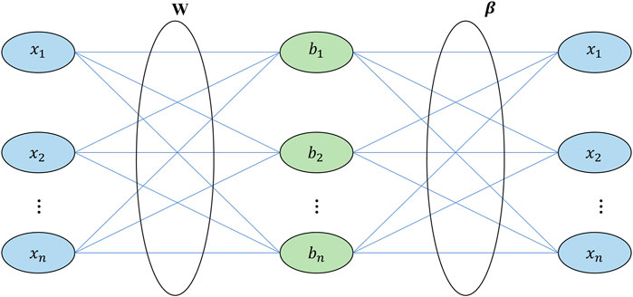
FIGURE 1. Structure of extreme learning machine. W is input weight, $\beta$ is output weight.

If Eq. 5 is solved by the gradient learning method, it can be used to represent all parameters, and the iteration can be written as given in Eq. 7.

${\theta }_k={\theta }_{k-1}-\eta \frac{\partial E\left(\theta \right)}{\partial \theta },(7)$

where $\eta$ is the learning efficiency. For feedforward neural networks, back-propagation neural networks are generally used. The neural network is a multilayer feedforward network trained according to error (You et al., 2021). The neural network includes input layer nodes, output layer nodes, and one or more hidden layer nodes. First, the input signal reaches the hidden layer node, where it passes through the excitation function and the output signal of the hidden layer node is then transmitted to the output node to finally get the output result. (Fukui and Kawakami, 1986). The learning process is that the neural network constantly changes the connection weight of its own network in the case of external input samples, so as to make the output result of the network closest to the expected output value (Xiong et al., 2018). If the output results differ greatly from the expected values, backpropagation can be carried out, and then the weights of each neuron can be modified again, and finally, a good classifier can be trained through continuous iteration. If the learning rate is too small, the learning speed is very slow. If the selection is too large, it is difficult to obtain network convergence. If Eq. 6 is a non-convex function, it is easy to fall into a local minimum by continuously iterating and adjusting parameters. Repeated iteration is not only time consuming but also easily falls into the situation of learning and fitting (Lcfcbvre, 2014).

In SLFNs, W and b are given at the beginning of the algorithm and can be arbitrarily specified. Then, H is calculated, while the value remains unchanged. In this way, only the parameter $\beta$ that can be changed is left, and this shows that the given W and b do not affect the results.

When W and b are fixed, Eq. 4 is solved by replacing it with Eq. 8:

$\parallel H\widehat{\beta }-T\parallel =\mathit{min}\parallel H\beta -T\parallel .(8)$

The least squares solution can be obtained by solving the Eq. 8.

In some large-scale projects, the learning process usually uses all the data and these learning times are very long. If new samples are added at this time, they have to learn together with the original data. In this way, it is a waste of time to relearn all the data. The online sequential learning neural network (OS-LNN) does not have to learn the previous data, but only has to add the new data to the learned network. However, the OS-LNN has to set network weights, and the training speed is also very slow. Although the training is completed, the online sequential learning–extreme learning machine (OS-ELM) can not only learn data one by one but also learn them batch by batch. The least squares solution of $H\beta -T$ is $\widehat{\beta }=H^{*}T$, and we considered that $Rank\left(H\right)=\stackrel{\sim }{N}$ is the number of hidden layer units, and $H^{*}$ is the left pseudo inverse of H, $H^{*}H=I_N$.

$H^{*}={\left.{\left(H\right.}^{T}H\right)}^{-1}H.(9)$

By substituting equation (9) into equation (8), we get

${\left.{\widehat{\beta }=(H}^{T}H\right)}^{-1}HT.(10)$

According to previous studies (Dac and Trung, 2023; Ma et al., 2023), the least square root is ${\beta }^{\left(0\right)}=K_0^{-1}{H}_{0}T$, where $K_0=H_0^T{H}_0$. When adding the new data (k + 1), $N_{k+1}={\left\{x_i,t_i\right\}}_{i=({\displaystyle \sum }_{j=0}^k{N}_j)+1}^{{\sum }_{j=0}^{k+1}{N}_j}$, $k\ge 0,N_{k+1}$ is (k+1)^th data, $K_{k+1}=K_k+H_{k+1}^T{H}_{k+1}$, and

${\beta }^{\left(k+1\right)}={\beta }^{\left(k\right)}+K_{k+1}^{-1}{H}_{k+1}^T\left(T_{k+1}-H_{k+1}{\beta }^{\left(k\right)}\right).(11)$

With the help of the Sherman-Morrison-Woodbury (SMW) equation, ${\beta }^{\left(k+1\right)}$ can be calculated by

${\beta }^{\left(k+1\right)}={\beta }^{\left(k\right)}+P_{k+1}{H}_{k+1}^T\left(T_{k+1}-H_{k+1}{\beta }^{\left(k\right)}\right).(12)$

where ${P_{k+1}=K}_{k+1}^{-1}=P_k-P_k{H}_{k+1}^T{\left(I+H_{k+1}{P}_k{H}_{k+1}^T\right)}^{-1}\times H_{k+1}{P}_k$.

When the OS-ELM faces the new data, it does not have to relearn the old data, which makes it faster than the other neural network methods. When selecting the network parameters, it becomes only necessary to determine the number of neural units in the hidden layer, which also reduces the dependence on the network layers.

The whale optimization algorithm is mainly divided into three steps: surround prey, spiral bubble net attack method, and randomly search for prey.

Surround prey: because the location of the target prey is unknown a priori, the WOA algorithm treats the location of the best candidate in the current whale group as the location of the target prey, and the other individuals in the whale group update the location according to the location of the best candidate:

$D=\left|C\bullet X^{*}\left(t\right)-X\left(t\right)\right|,(13)$

$X\left(t+1\right)=X^{*}\left(t\right)-A\bullet D,(14)$

$A=2ar-a,(15)$

$C=2r,(16)$

where X is the position vector of the current solution; t is the number of iterations; A and C are coefficient vectors; $X^{*}$ is the position vector of the optimal solution in the current whale population. a decreases linearly from 2 to 0 as the number of iterations increases; r is an arbitrary vector between 0 and 1.

Spiral bubble net attack method: the WOA algorithm first calculates the distance between the individual whale and the target prey, and then simulates the spiral movement of humpback whales for hunting behavior:

$D^{\prime }=\left|X^{*}\left(t\right)-X\left(t\right)\right|,(17)$

$X\left(t+1\right)=D^{\prime }{e}^{bl}\cos \left(2\pi l\right)+X^{*}\left(t\right),(18)$

where b is the constant coefficient defining the spiral shape, and l is a random number in the interval [−1, 1].

Randomly search for prey: in the process of predation, when A is greater than 1 or less than −1, the individuals in the whale group randomly select a prey with reference to each other’s position to improve the global search ability of the algorithm, namely,

$D=\left|C{X}_{rand}-X\right|,(19)$

$X\left(t+1\right)=X_{rand}-AD,(20)$

where $X_{rand}$ is a randomly selected position vector for the current whale group.

The steps for WOA to optimize the ELM are as follows:

(1) Parameter initialization. Set the WOA parameters, namely, the number of whales, maximum iterations, variable dimensions, and upper and lower limits of variables;

(2) Population initialization. Randomly initialize the position values of each dimension of all whale individuals, and the position values of each dimension of each whale individual representing the input weights or thresholds;

(3) Calculate the fitness value. Select the objective function to calculate the fitness value of each whale individual;

(4) Update the optimal solution. According to the fitness value of each whale individual, find the position of the optimal solution in all solutions and update the position of each whale individual according to the position of the optimal solution;

(5) The position of each individual whale is updated. When the probability p < 0.5 and | A |<1, the location is updated according to Equation 16. If | A | ≥ 1, a location vector X_rand is randomly selected and the location is updated according to Equation 19. when the probability p ≥ 0.5, the location is updated through Equation 20.

3.2 Wavelet packet energy entropy extraction

The structure of the wind solar storage microgrid system is shown in Figure 2.

FIGURE 2

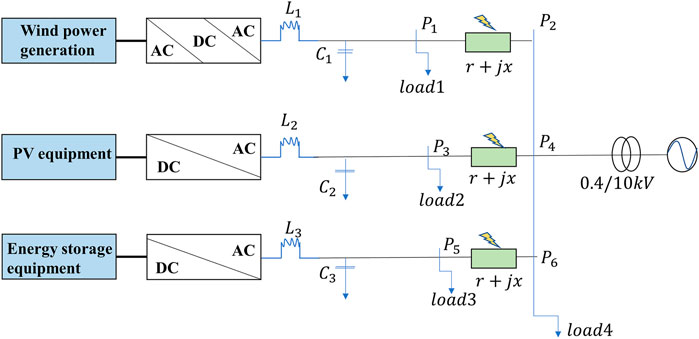
FIGURE 2. Structure of microgrid system. L₁, L₂, and L₃ are filter inductances; C₁, C₂, and C₃ are filter capacitors; Load1, Load2, Load3, and Load4 are electrical loads; r is line resistance; x is line reactance.

The internal line faults of the microgrid can be divided into single-phase ground short circuit (AG, BG, and CG), two-phase short circuit (AB, AC, and BC), two-phase ground short circuit (ABG, ACG, and BCG), three-phase short circuit (ABC), and three-phase ground short circuit (ABCG) faults.

When processing the signal, wavelet packet decomposition can decompose the low-frequency component and high-frequency component of the signal at the same time; higher the resolution, more detailed the decomposition and better the effect. The square-integrable function f(t) can be decomposed into a scaling function $\varphi \left(t\right)$ and wavelet function $\phi \left(t\right)$; $\varphi \left(t\right)$ is low frequency of f(t), $\phi \left(t\right)$ is high frequency of f(t), and their relationship includes

$\left\{\begin{array}{c}{\delta }_{2n}\left(t\right)=\sqrt{2}{\displaystyle \sum }_{k\in z}h\left(k\right){\delta }_n\left(2t-k\right)\\ {\delta }_{2n+1}\left(t\right)=\sqrt{2}{\displaystyle \sum }_{k\in z}g\left(k\right){\delta }_n\left(2t-k\right)\end{array}\right.,(21)$

where $h\left(k\right)$ is low pass filter coefficient, and $g\left(k\right)$ is high pass filter coefficient.

When $n=0,{\delta }_0\left(t\right)=\varphi \left(t\right),{\delta }_1\left(t\right)=\phi \left(t\right),$ the set of functions defined above {${\delta }_n\left(t\right)$} (n = 0,1,2,...) is determined by ${\delta }_0\left(t\right)=\varphi \left(t\right)$ determined wavelet packet. According to the fast algorithm of orthogonal wavelet transform, the recursive formula of wavelet packet coefficients can be obtained as follows:

$\left\{\begin{array}{c}{\lambda }_{i+1}^{2i}={\displaystyle \sum }_{k\in z}h\left(k-2t\right){\lambda }_i^j\left(k\right)\\ {\lambda }_{i+1}^{2i+1}={\displaystyle \sum }_{k\in z}g\left(k-2t\right){\lambda }_i^j\left(k\right)\end{array}\right.,(22)$

where ${\lambda }_i^j\left(k\right)$ is the kth coefficient corresponding to the jth node of layer i after wavelet packet decomposition.

Wavelet packet energy entropy is a description of signal uncertainty, which can reflect the degree of random change of signals. When a fault occurs in the internal lines of the microgrid, because the voltage signal contains non-stationary signal components, the wavelet packet voltage reconstruction signal waveform will immediately fluctuate at the time of the fault. The wavelet packet decomposition and reconstruction technology can make accurate and rapid localization analysis of the voltage signal, which is reflected in the wavelet packet energy entropy, so the wavelet packet energy entropy can well reflect the fault characteristics of the voltage signal. According to information entropy theory, wavelet packet energy entropy can be defined as

$WPEE=-{\sum }_{i=1}^{L}P\left(X_{i,j}\right){\mathit{log}}_{2}P\left(X_{i,j}\right),(23)$

where L is the original signal length; X_{i, j} is the jth decomposition signal of layer i; P (X_{i, j}) is the frequency band energy probability density, and the mathematical expression is

$P\left(X_{i,j}\right)=\frac{E_{i,j}}{{\sum }_{j=1}^{2^i}{E}_{i,j}},(24)$

where E_i,j is the energy of the jth decomposed signal of the ith layer, defined as

$E_{i,j}={\displaystyle \sum }_{k=1}^N{\left|{\lambda }_i^j\left(k\right)\right|}^2,(25)$

where N is the length of the jth frequency band.

3.3 Data

According to Figure 2, a microgrid model that includes wind turbine (10 kW), photovoltaic cell (10 kW), and battery (10 Ah) is built in the MATLAB simulink environment. The filter inductances L₁, L₂, and L₃ are 3.6e⁻³ H; the filter capacitors C₁, C₂, and C₃ are 200e⁻⁶ F; the electrical loads Load1, Load2, Load3, and Load4 are 10 kVA, 10 kVA, 5 kVA, and 15 kVA, respectively; the line resistance r is 0.175 Ω/km; and the line reactance x is 0.070 Ω/km. Simulate each type of line fault at 10%, 20%, 30%, 40%, 50%, 60%, 70%, 80%, and 90% of the lines between P₁ and P₂ on the microgrid side. The db6 wavelet is selected as the wavelet base, and the simulated A-phase fault voltage is analyzed by three-layer wavelet packets to obtain 2³ sub signals in different frequency bands, which are reordered from low frequency to high frequency. The wavelet packet signal reconstruction is carried out for each frequency band, and a total of eight wavelet packet reconstruction signals are obtained. The energy entropy of the reconstructed signal of each wavelet packet is calculated, and a set of eigenvectors are constructed from the energy entropy of eight wavelet packets. By the same processing of phase B and phase C voltage signals, a eigenvector containing 24 wavelet packet energy entropy can be obtained $X={\left[x_1,x_2,\dots ,x_{24}\right]}^T$. Taking $X={\left[x_1,x_2,\dots ,x_{24}\right]}^T$ as the input sample of the network, and the output sample of the network is $T={\left[t_1,t_2,\dots ,t_4\right]}^T$, t₁, t₂ and t₃, respectively, representing the line status of phase A, phase B, and phase C, and t₄ representing whether the fault phase is grounded when the line fails. When it is 0, it means there is no fault or the fault phase is not grounded at this time; when the output is 1, it means the fault phase is grounded.

The data samples at 10%, 20%, 40%, 60%, 80%, and 90% of the line positions are taken as training samples, and the data samples at 30%, 50%, and 70% are taken as test samples. The number of neurons in the input layer of ELM is 24, the number of neurons in the output layer is 4, the number of neurons in the hidden layer is determined to be 35 according to the trial and error method, the number of whales in WOA is 30, the maximum number of iterations is 200, and the variable dimension is 875.

4 Results and discussion

4.1 Fault detection based on original ELM coupled with distance selection

As shown in Table 1, the method proposed in this article is nearly twice (mean error is 0.47%) as good as the method using B2 data only (mean error is 1.48%). The performance based on B2 only is better than that based on B1 (4.58%), it should be noted that the performance using combined B1B2 data (4.0%) is the poorest among the all methods.

TABLE 1

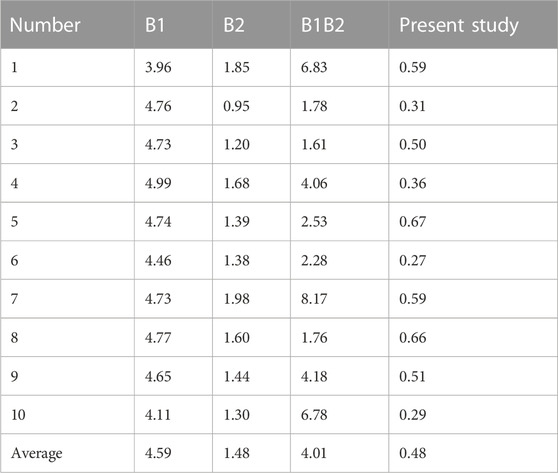
TABLE 1. Test error in the experiments (%).

We compared the results between actual and predictive in Figure 3, a total of samples of 209 are used for testing. Only 21 samples is not completely positioned accurately, that is, 10% samples have positioning errors, and the predicted values of the remaining test samples are identical to the actual values. The maximum error is that the actual value is 85% of the fault point that away from B1 and the predicted value is 92% of the fault point, with 7% error.

FIGURE 3

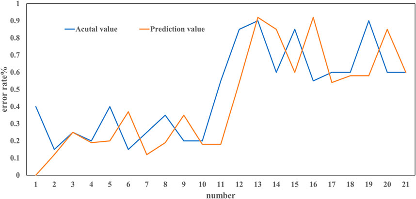
FIGURE 3. Comparison between actual values and predictive value.

We did a comparative experiment, and the results are presented in Figure 4, when the B1 fault occurs, the data of B1 and B2 are used to locate the fault location. Through comparison, it can be found that the data on the B1 side should be accurate to the data on the B2 side. Table 2 divides the fault distance into three sections: 0%–33%, 33%–66%, and 66%–100%, respectively. Then, only the data of B1 is used to locate the fault, and it is found that the farther away from B1, the greater the test error. We demonstrated that it is more effective to use data close to the fault point. From the experimental results, it is shown that using the data points at the near end has better results. The farther the signal is transmitted, the greater is the resistance affected by various electrical components.

FIGURE 4

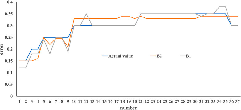
FIGURE 4. Comparison of experimental values with B1 and B2 data when fault is close to B1 end.

TABLE 2

TABLE 2. Distance interval testing error through B1 data.

The experiment in Table 3 uses the SVM classifier, random forest (RF), and recurrent neural network (RNN) to test the method proposed in this article. Moreover, we choose to use libsvm and genetic the algorithm to optimize C and gamma parameters. The range of C is 0–1,000, the range of gamma is 0–1,000, the maximum evolutionary algebra is 200, and the maximum data of the population is 20. We can see that, in our methods, the selection of data based on the fault distance coupled with SVM can improve the accuracy of detection of fault in smart grids, with an average error of 0.86%, followed by RF with a mean error of 0.91% and B1B2-SVM with a mean error of 0.98%. Keeping the results of Figure 4 in mind when coupling with the SVM algorithm, the B1B2 method can obtain substantial accuracy with an average error of 0.98%, B1+SVM has the poorest performance with a mean error of 3.87%, B2+SVM has a moderate performance with a mean error of 1.61% (ranking of performance in Figure 4 is B2 > B1B2 > B1), which means that the artificial intelligence algorithm (SVM here) can substantially improve the detection of fault in the smart grid. the SVM can improve accuracy of fault detection more robustly than RF and RNN, for example, B1+RF has an error of 4.3%, followed by B1+RNN with 3.8%, and 1.9% and 2.0% for B2+RF and B2+RNN, respectively; 1.4% and 1.1% for B1B2+RF and B1B2+RNN, respectively. Fault distance–based data selection can substantially improve accuracy of fault detection on the basis of not only SVM but also RF and RNN, for example, 0.8%, 0.9%, and 1.2% for SVM, RF, and RNN, respectively, which means the fault distance–based data selection is useful for fault diagnoses.

TABLE 3

TABLE 3. Experimental results of SVM (%).

After processing the data with Daubechies wavelet, the data output of the first layer is selected as the feature of the input classifier. The results obtained after positioning with ELM and with SVM, RF, and RNN are shown in Figures 5, 6, respectively. It can be seen that the method proposed in this article still has a good effect, with an average error of 0.66%. The method of B1+ELM after wavelet transform is the poorest with a mean error of 5.12%, followed by B1B2+ELM with of mean error of 4.93% and B2+ELM with a mean error of 3.72. Performance of the SVM, RF, and RNN methods after wavelet transform is better than that of the ELM method, and the SVM has the best performance. As we can see in Figure 6, B1+SVM, B2+SVM, or B1B2+SVM has smaller errors in fault detection, specifically, B1+SVM has the poorest performance with a mean error of 4.7%, followed by B2+SVM (1.98%), B1B2+SVM (1.14%), and our method, i.e., fault distance–based data selection + SVM (0.96%), which means that our fault distance–based method to detect faults is robust. The methods of both RF and RNN are poorer than SVM; B1+RF and B1+RNN are the poorest with a mean 5.04% and 3.9%, respectively. However, RF and RNN substantially improve the accuracy of fault detection, which is still poorer than SVM, for example, a mean error of 1.099% and 1.26% for the fault distance–based data selection + RNN and fault distance–based data selection + RF, respectively, while the mean error was 0.959% for our method, which means that improvement of SVM is robust.

FIGURE 5

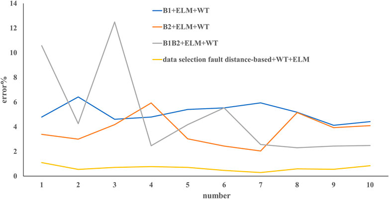
FIGURE 5. Data are located by ELM after wavelet transform.

FIGURE 6

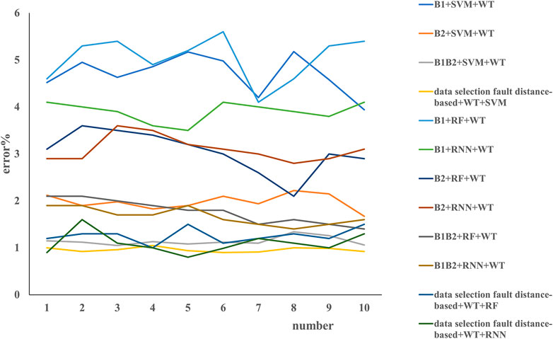
FIGURE 6. Data are located by SVM, RF, and RNN after wavelet transform.

4.2 Fault detection based on WOA-ELM method

In order to verify the superiority of the WOA-ELM diagnostic model and improve the recognition accuracy, the WOA-ELM diagnostic model is compared with the traditional ELM diagnostic model and optimized ELM by Quantum PSO, i.e., PSO-ELM. The results are shown in Figure 7. The error of WOA-ELM and WOA-ELM diagnostic faults are nearly 8.5% and 8.9%; separately, they are higher than the traditional ELM model with an error of 11%. We further compared the results of the three models using the mean square error (MSE), root mean square error (RMSE), and mean absolute error (MAE) (Table 4). The WOA-ELM model is largely better than the PSO-ELM and ELM models both in the training and testing data sets in fault detection. The WOA-ELM model uses WOA algorithm to optimize the input weight and hidden layer node threshold of the ELM, overcomes the shortcomings of random initialization of the input weight and hidden layer node threshold of the ELM, improves the global search ability of the network, and makes the network have better recognition accuracy.

FIGURE 7

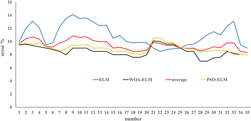
FIGURE 7. Comparative results of WOA-ELM, PSO-ELM, and traditional ELM models.

TABLE 4

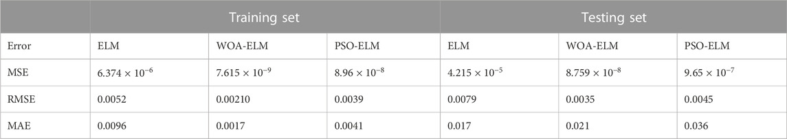
TABLE 4. Error between ELM and WOA-ELM methods in training and testing data sets.

Compared with the research results of others, the literature (Ji et al., 2022) proposes a basic network architecture design, using a simplified residual connection technology, using focal loss as the objective function for supervised training, adding a BatchNormalization layer to the network for optimization, reducing parameters based on ShuffleNet network, and improving accuracy on the basis of the attention mechanism, a process that can automatically determine the appropriate CNN architecture for fault diagnosis problems. Wang et al. (2011) proposed a new method for fault identification on the basis of parameter optimized variational mode decomposition (VMD) and convolutional neural network (CNN). Luo et al. (2014) proposed a real-time deep learning algorithm to classify and localize the faults that occurred in the system based on measured data. Luo et al. (2017) presented a method on the basis of gated graph neural network for automatic fault localization on distribution networks. The method aggregates problem data in a graph where the feeder topology is represented by the graph links and nodes attributes that can encapsulate any selected information such as operated devices, electrical characteristics, and measurements at the point. Kasun et al. (2013), Zhibin et al. (2019), and Xue and Dola (2022) proposed a multi-fault diagnosis model of distribution network on the basis of the fuzzy optimal convolutional neural network. In order to compare their results with ours, we used the RBF neural network and BP neural network to detect fault location in the smart grid and used indicators of MSE, RMSE, and MAE to evaluate accuracy; the results are provided in Table 5.

TABLE 5

TABLE 5. Error between BP and RBF methods in training and testing data sets.

The three training errors of the WOA-ELM model are about one order of magnitude smaller than those of the BP neural network model and ELM model, while the three training errors of the RBF neural network model are 6–13 orders of magnitude smaller than those of the WOA-ELM model. The training effect of RBF neural network is the best. However, it can be seen from Table 6 that the three test errors of the WOA-ELM model are significantly smaller than those of the RBF neural network model. It shows that the RBF neural network model has a phenomenon of over-fitting, and its generalization ability is weak and cannot accurately identify the untrained fault types.

TABLE 6

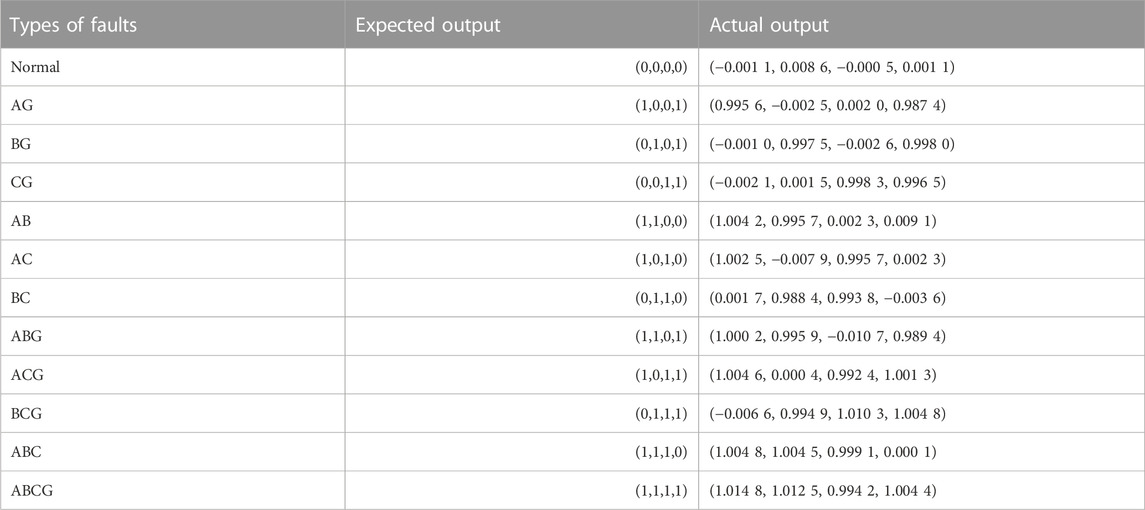
TABLE 6. Fault diagnosis results of test samples at 50% of line.

4.3 WOA-ELM performance in microgrid fault diagnoses

In substituting the data samples into the WOA-ELM fault diagnosis model for training and testing, the line fault diagnosis results of the test samples at 50% of the line position are shown in Table 6.

It can be seen from Table 6 that the absolute value of the error between the expected output and the actual output of the WOA-ELM fault diagnosis model does not exceed 0.015 at the most. The error is small, the accuracy is high, and the approximation ability is strong. It can accurately identify the fault types of microgrid lines.

In order to verify that WOA-ELM diagnostic model has better performance and higher recognition accuracy than the other models, the BP neural network, RBF neural network, and ELM were selected to establish the diagnostic models for comparative analysis. The expected output and actual output results of all training samples (72) are shown in Figure 8A. It can be seen from Figure 8A that the training error of the BP neural network model is large; the training results of the other three models can well approximate the expected output; the error between the actual value and expected value is small; and the training accuracy is high.

FIGURE 8

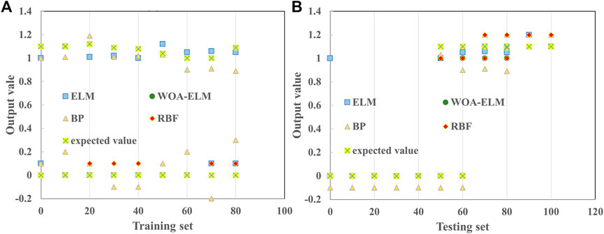
FIGURE 8. Desired output and actual output of 72 training samples (A) and testing samples (B).

The expected output and actual output results of all test samples (36) are shown in Figure 8B. It can be seen from Figure 8B that the test results of the BP neural network model, RBF neural network model, and the non-optimized ELM model have large errors, while the test accuracy of the WOA-ELM model is the highest.

5 Conclusion

In this article, a microgrid fault diagnosis method based on the whale algorithm optimization limit learning machine was proposed. The whale algorithm has the characteristics of fast convergence speed and strong global optimization ability. It optimizes the input weights and hidden layer neuron threshold of the ELM, effectively avoids the shortage of random initialization of network input weights and hidden layer threshold, enhances the approximation ability of the model, and significantly improves the recognition accuracy of the network. The results show that the selection of data based on the fault distance is twice as effective as the useless real data. The ELM method was proved to have a good location result by using the support vector machine classifier and wavelet transform to process the signal. After the ELM is improved by the WOA algorithm, the accuracy of fault detection is improved by nearly 22.5%. The simulation results show that the WOA-ELM model has a higher recognition accuracy than the BP neural network model, RBF neural network model, and ELM model and can more accurately identify the fault types of internal lines in the microgrid, which verifies the effectiveness and reliability of the WOA-ELM model.

The power system simulated in this article may be different from the complex power grid in reality. The actual power system wires are more complex, and the accuracy of the detection data may not be as high. Now, the method proposed in this article is to choose which end of the data to use on the basis of the distance. In fact, in the power system model, the information of the power components on both sides is not equal, which leads to a worse situation when using only the B1 end data than when using only the B2 end data. In this article, we use distance 1:1 to select data. Next, we can select data at B1 or B2 on the basis of a certain proportion, such that the effect of adding distance to power components is equivalent to 1:1. In fault location, many articles use wavelet transform to analyze because when a fault just occurs, the power system will produce transient signals, which is also one of the directions of future research. How to select data for fault location? Is it a half cycle or one cycle after fault? How long to choose is also something that can be further studied in the future.

Data availability statement

The original contributions presented in the study are included in the article/Supplementary Material; further inquiries can be directed to the corresponding author.

Author contributions

Conceptualization: FX and YL; methodology: YL; software: FX; validation: FX and YL; formal analysis: LW; investigation: LW; resources: FX; data curation: LW; writing—original draft preparation: FX; writing—review and editing: YL; visualization: FX; supervision: FX; project administration: YL; funding acquisition: YL; all authors have read and agreed to the published version of the manuscript.

Acknowledgments

The authors of the present study thank the reviewers for their contribution in improving the study.

Conflict of interest

Author FX was employed by State Grid Yantai Fushan Power Supply Company.

The remaining authors declare that the research was conducted in the absence of any commercial or financial relationships that could be construed as a potential conflict of interest.

Publisher’s note

All claims expressed in this article are solely those of the authors and do not necessarily represent those of their affiliated organizations, or those of the publisher, editors, and reviewers. Any product that may be evaluated in this article, or claim that may be made by its manufacturer, is not guaranteed or endorsed by the publisher.

References

Ayushi, C., Preeti, G., Singh, G. N., and Moy, C. J. (2022). Performance analysis of an optimized ANN model to predict the stability of smart grid. Complexity 2022, 1–13. doi:10.1155/2022/7319010

CrossRef Full Text | Google Scholar

Chang, N., Song, G., Hou, J., and Chang, Z. (2023). Fault identification method based on unified inverse-time characteristic equation for distribution network. Int. J. Electr. Power Energy Syst. 20, 213–223. doi:10.1016/J.IJEPES.2022.108734

CrossRef Full Text | Google Scholar

Chen, B., Yu, L., Luo, W., Wu, C., Li, M., Tan, H., et al. (2022). Hybrid tree model for root cause analysis of wireless network fault localization. Web Intell. 20 (3), 213–223. doi:10.3233/web-220016

CrossRef Full Text | Google Scholar

Chen, L., Jiang, Y., Deng, X., Chen, H., and Zheng, S. (2022). A novel fault recovery method of active distribution networks oriented to improving resilience. Energy Rep. 8 (S15), 456–466. doi:10.1016/j.egyr.2022.10.152

CrossRef Full Text | Google Scholar

Dac, Q. H., and Trung, H. H. (2023). Solving partial differential equation based on extreme learning machine. Math. Comput. Simul. 205, 697–708. doi:10.1016/j.matcom.2022.10.018

CrossRef Full Text | Google Scholar

Fang, J., Wang, H., Yang, F., Yin, K., Lin, X., and Zhang, M. (2022). A failure prediction method of power distribution network based on PSO and XGBoost. Aust. J. Electr. Electron. Eng. 19 (4), 371–378. doi:10.1080/1448837x.2022.2072447

CrossRef Full Text | Google Scholar

Fukui, C., and Kawakami, J. (1986). An expert system for fault section estimation using information from protective relays and circuit breakers information from protective relays and circuit breakers. IEEE Trans. Power Deliv. PER-6 (04), 83–90. doi:10.1109/tpwrd.1986.4308033

CrossRef Full Text | Google Scholar

Hou, S., Xu, Y., and Guo, W. (2022). Distribution network fault-line selection method based on MICEEMDAN–recurrence plot–yolov5. Processes 10 (10), 2127. doi:10.3390/pr10102127

CrossRef Full Text | Google Scholar

Ji, Q., Hu, Z., and Liu, X. (2022). Fault Diagnosis algorithms of distribution network based on convolutional neural network. J. Phys. Conf. Ser. 2301 (1), 012009. doi:10.1088/1742-6596/2301/1/012009

CrossRef Full Text | Google Scholar

Jia, Y., Liu, Y., Wang, B., Lu, D., and Lin, Y. (2022). Power network fault location with exact distributed parameter line model and sparse estimation. Electr. Power Syst. Res. 212, 108137. doi:10.1016/j.epsr.2022.108137

CrossRef Full Text | Google Scholar

Kasun, L. L. C., Zhou, H., Huang, G., and Vong, C.-M. (2013). Representational learning with extreme learning machine for big data. IEEE Intell. Syst. 28 (06), 31–34.

Google Scholar

Lcfcbvre, D. (2014). On-line Fault Diagnosis with partially observed Petri ncts. IEEE Transaction Automatic Control 59 (07), 1919–1924. doi:10.1504/IJISE.2018.10016217

CrossRef Full Text | Google Scholar

Lei, J., Guo, Y., Luo, D., Xu, Z., and Wang, R. (2022). Fault Location of distribution network based on multi-population particle swarm optimization algorithm. J. Phy. Conf. Ser. 2360 (1), 012024. doi:10.1088/1742-6596/2360/1/012024

CrossRef Full Text | Google Scholar

Li, Z., Qiao, J., Wang, Y., and Yin, X. (2022). A faulty section location method for distribution grid based on grounding fault transfer device. Energy Rep. 8 (S8), 81–89. doi:10.1016/j.egyr.2022.09.088

CrossRef Full Text | Google Scholar

Liu, Y., Zhang, S., Li, L., Wang, S., Lu, T., Yu, H., et al. (2022). A machine learning-based fault identification method for microgrids with distributed generations. J. Phy. Conf. Ser. 2360 (1), 012019. doi:10.1088/1742-6596/2360/1/012019

CrossRef Full Text | Google Scholar

Luo, J., Vong, C. M., and Wong, P. K. (2017). Sparse bayesian extreme learning machine for multiclassification. IEEE Trans. Neural Netw. Learn. Syst. 25 (04), 836–843. doi:10.1109/TNNLS.2013.2281839

CrossRef Full Text | Google Scholar

Luo, Y., Ling, S., and Cao, Y. (2014). Fault diagnosis of electric power grid based on improved RBF neural network. TELKOMNIKA Indonesian J. Electr. Eng. 12 (09), 4777–4784. doi:10.11591/telkomnika.v12i9.4642

CrossRef Full Text | Google Scholar

Ma, T., Hu, Z., Xu, Y., and Dong, H. (2022). fault location based on comprehensive grey correlation degree analysis for flexible DC distribution network. Energies 15 (20), 7820. doi:10.3390/en15207820

CrossRef Full Text | Google Scholar

Ma, Z., Wang, X., and Hao, Y. (2023). Development and application of a hybrid forecasting framework based on improved extreme learning machine for enterprise financing risk. Expert Syst. Appl. 215, 119373. doi:10.1016/j.eswa.2022.119373

CrossRef Full Text | Google Scholar

Shafiullah, M., AlShumayri Khalid, A., and Alam, M. S. (2022). Machine learning tools for active distribution grid fault diagnosis. Adv. Eng. Softw. 173, 2022. doi:10.1016/J.ADVENGSOFT.2022.103279

CrossRef Full Text | Google Scholar

Singhal, D., Ahuja, L., and Seth, A. (2022). An insight into combating security attacks for smart grid. Int. J. Perform. Eng. 18 (7), 512. doi:10.23940/ijpe.22.07.p6.512520

CrossRef Full Text | Google Scholar

Waldrigues, B. N., Matos, C. M. S., Frizzo, S. S., and Quietinho, L. V. R. (2022). Wavelet LSTM for fault forecasting in electrical power grids. Sensors 22 (21), 8323. doi:10.3390/s22218323

PubMed Abstract | CrossRef Full Text | Google Scholar

Wang, J., Zhou, L., Hong, H., and Zhang, G. X. (2011). An extended spiking neural P system for fuzzy knowledge representation. Int. J. Innovative Comput. Inf. Control 7 (7A), 3709–3724. doi:10.1049/iet-cta.2010.0325

CrossRef Full Text | Google Scholar

Wang, N. (2022). Fault line selection of power distribution system via improved bee colony algorithm based deep neural network. Energy Rep. 8 (S12), 43–53. doi:10.1016/j.egyr.2022.10.070

CrossRef Full Text | Google Scholar

Xin, C. (2022). Research on high-frequency information-transmission method of smart grid based on CNN-LSTM model. Information 13 (8), 375. doi:10.3390/info13080375

CrossRef Full Text | Google Scholar

Xiong, G., Shi, D., and Zhang, J. (2018). A binary coded brain storm optimization for fault section diagnosis of power systems for fault section diagnosis of power systems. Electr. Power Syst. Res. 163 (01), 441–451. doi:10.1016/j.epsr.2018.07.009

CrossRef Full Text | Google Scholar

Xue, W., and Dola, S. (2022). “KNEW: Key generation using NEural networks from wireless channels,” in Proceedings of the 2022 ACM Workshop on Wireless Security and Machine Learning (WiseML '22) (New York, NY, USA: Association for Computing Machinery), 45–50.

Google Scholar

Yan, X., Liu, R., Tu, N., and Xing, J. (2022). Research on fault location of distribution network with DG based on HHO. Sci. Discov. 10 (5). doi:10.11648/J.SD.20221005.19

CrossRef Full Text | Google Scholar

You, B., Qi, H., Ding, L., Li, S., Huang, L., Tian, L., et al. (2021). Fast neural network control of a pseudo-driven wheel on deformable terrain. Mech. Syst. Signal Process. 152, 107478. doi:10.1016/j.ymssp.2020.107478

PubMed Abstract | CrossRef Full Text | Google Scholar

Yuvaraja, T., Irina, K., Hariprasath, M., Ramya, K., Ravi, A., and Ramesh, T. A. (2022). Diminution of smart grid with renewable sources using support vector machines for identification of regression losses in large-scale systems. Wirel. Commun. Mob. Comput. 2022, 1–11. doi:10.1155/2022/6942029

CrossRef Full Text | Google Scholar

Zhang, X., Ding, R., Wang, Z., Guo, Z., Liu, B., and Wei, J. (2023). Power grid fault diagnosis model based on the time series density distribution of warning information. Int. J. Electr. Power Energy Syst., 146. doi:10.1016/J.IJEPES.2022.108774

CrossRef Full Text | Google Scholar

Zhibin, Z., Liping, S., and Xuan, C. (2019). Labeled box-particle CPHD filter for multiple extended targets tracking. J. Syst. Eng. Electron. 30 (1), 57–67. doi:10.21629/JSEE.2019.01.06

CrossRef Full Text | Google Scholar