Field studies of PERC and Al-BSF PV module performance loss using power and I-V timeseries

We have studied the degradation of both full-sized modules and minimodules with PERC and Al-BSF cell variations in fields while considering packaging strategies. We demonstrate the implementations of data-driven tools to analyze large numbers of modules and volumes of timeseries data to obtain the performance loss and degradation pathways. This data analysis pipeline enables quantitative comparison and ranking of module variations, as well as mapping and deeper understanding of degradation mechanisms. The best performing module is a half-cell PERC, which shows a performance loss rate (PLR) of −0.27 ± 0.12% per annum (%/a) after initial losses have stabilized. Minimodule studies showed inconsistent performance rankings due to significant power loss contributions via series resistance, however, recombination losses remained stable. Overall, PERC cell variations outperform or are not distinguishable from Al-BSF cell variations.

1 Introduction

Silicon solar cell technology has undergone a large scale transition in the past few years. Traditional aluminum back-surface field cells (Al-BSF) have been replaced by a more modern cell design: the passivated emitter and rear cell (PERC) (Trube, 2022). As silicon makes up nearly 95% (Philipps, 2023) of the total PV market share, this represents a significant transition in the industry as a whole.

Al-BSF cells, as the name suggests, feature a continuous layer of aluminum at the back of the cell in contact with crystalline silicon, which creates a “back-surface field” that hinders minority carriers from reaching the rear contact up to a certain degree.

The back-surface field increases the performance of the cell, but the aluminum silicon interface is still an area of high recombination. PERC cells normally have a passivated rear side with a grid of local aluminum contacts across the rear surface, as opposed to the continuous aluminum layer in Al-BSF. The limited aluminum-silicon contacts are still able to maintain the beneficial back-surface field while the passivated region significantly reduces the recombination at the rear of the cell. PERC cells offer a higher conversion efficiency than Al-BSF and better maintain performance with thinner wafers, allowing more cells to be produced from a given amount of raw material. The similar architecture between PERC and Al-BSF allows PERC to be integrated into industrial Al-BSF workflows without much disruption. Many efforts have been made to increase the cell efficiency of PERC (Kashyap et al., 2022a; Kashyap et al., 2022b; Kashyap et al., 2022c; Kashyap et al., 2022d; Kashyap et al., 2022e). Also, PERC cells are able to be made bifacial (Deline et al., 2019). This has led to new types of white rear side encapsulants designed to scatter light that passes between cells into the rear of the cell, increasing the energy yield (López-Escalante et al., 2018).

This rapid industry transition leads to a lack of long term data on PERC cells, especially in comparison with Al-BSF. Initial testing of PERC has shown that it does have unique degradation considerations. PERC cells are known to be more susceptible than Al-BSF to certain light based sources of degradation like light induced degradation (LID), including boron-oxygen related light induced degradation (BO-LID) (Jordan et al., 2022; Ino et al., 2023; Ding et al., 2022; Fokuhl et al., 2021; Lindroos and Savin, 2016) and light and elevated temperature induced degradation (LeTID) (Karas et al., 2023; Krauss et al., 2015; Kersten et al., 2015; Fokuhl et al., 2019; Fokuhl et al., 2021). Knowing this, studies of outdoor exposure of PERC modules in comparison with Al-BSF are important in understanding reliability concerns as the transition to PERC cells occurs.

Prior studies on comparing the degradation observed between PERC and Al-BSF cells have either solely examined full-sized modules that were exposed to outdoor conditions in the field (Theristis et al., 2023; Jordan et al., 2022), which were often commercially manufactured and lacked the capacity for tailoring cell packaging strategies, or solely conducted accelerated aging tests on minimodules indoors (Wang et al., 2019; Braid et al., 2018).

This study consists of outdoor exposure of full-sized modules of PERC and Al-BSF and minimodules of the same cell types with variants of packaging material and cell type. The (Current-Voltage) I-V data collected at standard test conditions (STC) or in field were analyzed using open-source data analysis tools. We demonstrate that the data analysis pipeline is not only flexible enough to capture nonlinear performance degradation (Hashemi et al., 2020; French et al., 2021; Hashemi et al., 2021; Theristis et al., 2021; Lindig et al., 2022; Livera et al., 2022a), but also capable of extracting performance loss and changes in electrical features from I-V curves at outdoor conditions (Li et al., 2023; Meena et al., 2022; Jain et al., 2020; Livera et al., 2019). Furthermore, our pipeline can construct data-driven network models of degradation pathways, allowing for the comparison of degradation mechanism among different variants (Nalin Venkat et al., 2023). We conducted a comparative analysis of the degradation of PERC versus Al-BSF, full-sized modules versus minimodules, and the impact of packaging variations in field.

2 Methods and data sources

2.1 Full-sized modules and standard-test-condition (STC) I-V

The field trial (FT) system used Canadian Solar Inc. Commercial PERC and Al-BSF full-sized modules in a string configuration during outdoor exposure in Suzhou, China, located in a Cfa Köppen-Geiger climate zone, as shown in Figure 1. The cells were boron-doped. Arrangements of 9–12 modules were operated in series with each other, with one of the modules shorted during each exposure step for around 6 months. Power, current, and voltage were measured from the string during operation and the modules were taken down for indoor I-V at standard test conditions (STC) and electroluminescent (EL) measurements approximately every 6 months. Four different trials were ongoing with each trial being dedicated to a certain variant or model of PV module. The FT included modules with half- and full-cells, Al-BSF and PERC cells, all summarized in Table 1.

FIGURE 1

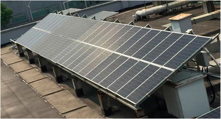
FIGURE 1. Field trial system using Canadian Solar Inc. Commercial full-sized modules during outdoor exposure in Shouzhu China.

TABLE 1

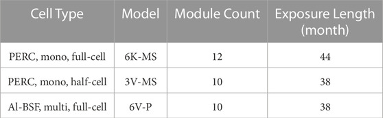
TABLE 1. Full-sized module variants in the field trial exposure.

2.2 Minimodules and field I-V

Sixteen 4-cell minimodules fabricated by Canadian Solar, Inc. were fielded at the SDLE SunFarm in Cleveland, OH. They were installed in July 2018 for continuous I-V and the maximum output power (P_MP) tracking. These 16 minimodules include boron-doped Al-BSF and PERC cells, and 4 different packaging strategies that include ethylene-vinyl acetate (EVA) and polyolefin (POE) encapsulants, and KPX and PPf backsheets from Cybrid Technologies. KPX is PVDF (polyvinylidene fluoride) based composite backsheet with outside layer K indicating Kynar^® PVDF, P standing for PET (Polyethylene terephthalate) core layer, and X meaning inner polymer layer with or without fluorine. PPf is PET-based composite backsheet with outside layer P meaning enhanced PET, core P standing for PET, and inner f representing fluorine polymer layer. KPX has a lower vapor transmission rate (VTR) as compared to PPf. The 4 variations of packaging were selected from the full set of minimodules (6 total packaging strategies) because they represent the extremes of the cell environment to be tested, while allowing for 2 modules of each type to be fielded for the remainder of the project. Minimodules were connected via 4-point electrical connection to Daystar Multi-Tracer Load Units for 10 min I-V curve tracing and 1 min P_MP data. This totals to a combined I-V sum of over 450,000 across all minimodules. Each minimodule also had continuous temperature data via a thermocouple located on the backsheet of each module. Two of the minimodules (the PERC cells with PPf backsheets) were taken down shortly after installation due to channel errors in the Daystar.

2.3 Data analysis tools

We propose a pipeline method that utilizes open-source data-driven R packages to not only analyze field Power and I-V outdoor data for performance loss degradation but also infer degradation pathways.

2.3.1 PVplr: performance loss rate analysis

The long term performance of PV systems in outdoor environments is usually quantified performance loss rate (PLR) (Jordan et al., 2016). The units of this metric are % per annum (%/a) or loss in power output per year of operation. The sign of this metric aligns with the direction of power change. A typical PLR calculation requires data filtering, model selection, outlier analysis, etc.

PVplr (Curran et al., 2020a; Curran et al., 2020b) is an R package (R Core Team, 2020) that allowed for the calculation of PLR with several different methods and parameters, as opposed to one universal method. This package makes it easy to test different filtering criteria and models to view the impact on a final PLR calculation. Comparisons between PLR methods showed that universal temperature corrections (the XbX + UTC model in PVplr) showed the most consistency and least uncertainty between results because it did not extrapolate temperature between seasonal periods, so this is the method that is used for all PLR calculations in this study.

Another benefit of the PVplr package is the unique ability to calculate non-linear PLR results using piecewise linear models. The piecewise linear model splits a model into linear components with different slopes which are bound by changepoints. While the number of changepoints must be supplied to the model, their values are determined automatically by the fitting algorithm and define where the slope changes occur within the model. This can be used to capture non-linear trends in PV data while still providing the interpretability of linear PLR results, which are the most common. Non-linear PLR is becoming more commonplace with the transition to PERC, given the greater susceptibility to LID and LeTID, which generally create a higher value of loss in a short period at the beginning of operation. Some module warranties have two rated PLR values; one for the first year and a different one for the following years.

2.3.2 ddiv: data-driven I-V feature extraction

The R package name ddiv (Huang et al., 2018a) stands for data driven I-V. The raw data of an I-V curve are the current and voltage values measured during the sweep. The number of measurements, or data points collected per I-V curve, depends on the device and setting used to take the curve, but higher resolution is generally better as it makes it easier to define the I-V trend. Typical numbers of data points include several hundreds to thousands, but can be as low as 40. The raw I-V curves themselves provide little quantitative information, but the parameters that can be extracted from them are desired for characterization. While some values, like the open-circuit voltage (V_OC), short-circuit current (I_SC), and maximum power can be pulled directly from the data given a high enough resolution, others require more complex analysis to extract. Series resistances (R_s) and shunt resistances (R_sh) require slope calculations at the start and end of the curves extrapolated down to, or near, the end points of the curve. Also, in cases with low resolution I-V curves, it becomes more likely that the actual maximum power will fall further between two measurements, leading to a lower than actual max power.

With indoor methods of I-V, tracing the machine software will typically provide feature results from measured curves, but this can be inconsistent between devices with different software. Additionally, outdoor I-V measurements are unlikely to have their features auto-reported at all. To account for problems like this, the ddiv package was developed to automatically extract I-V feature results from curves. The ddiv package uses spline fitting and moving regression to interpolate higher resolution curves and extract slopes from key points. It provides a consistent and automated way to extract results from curves from any source. It is particularly useful in outdoor I-V timeseries, having been demonstrated on datasets consisting of millions of I-V curves. The Suns-V_OC package uses this package as a dependency in its extraction of I-V features as well.

2.3.3 Suns-V_OC: reconstruct pseudo I-V curves for degradation and loss factors

The Suns-V_OC R package (Wang et al., 2020a) takes the concept of indoor Suns-V_OC measurements (Sinton and Cuevas, 2000) and applies it to outdoor I-V datastreams. Similar to power timeseries measurements, I-V timeseries collect I-V curves at set intervals, usually on the order of every 10 min, of modules under outdoor exposure. Being outdoors, there is much less control over the environment, with I-V curves being taken with significant variation in irradiance and temperature. Despite this variance in weather conditions, they can be corrected with enough data. I-V curves taken in a controlled indoor setting will typically have well controlled irradiance and temperature to ensure consistency between subsequent measurements, making comparisons easier and requiring less data overall.

V_OC measurements are taken with every I-V curve and can be corrected for temperature, leaving a series of V_OC measurements dependent on the outdoor irradiance when the curve was measured. The pseudo I-V curves can be built from these temperature corrected V_OC measurements taken over a range of outdoor irradiance. Once the ideal pseudo I-V curve has been built, the other I-V curves can be corrected to ideal conditions based on temperature and irradiance and compared to the ideal. The differences between the measured and ideal I-V curves provide information about mechanistic loss factors, just as with indoor Suns-V_OC characterization. By comparing the idealized and real curves, one can quantify specific loss parameters and directly observe the wattage lost for each one. The standard loss parameters quantified by this procedure are the uniform current, current mismatch, series resistance, and recombination losses. A visual of these loss parameters is given in Figure 2.

FIGURE 2

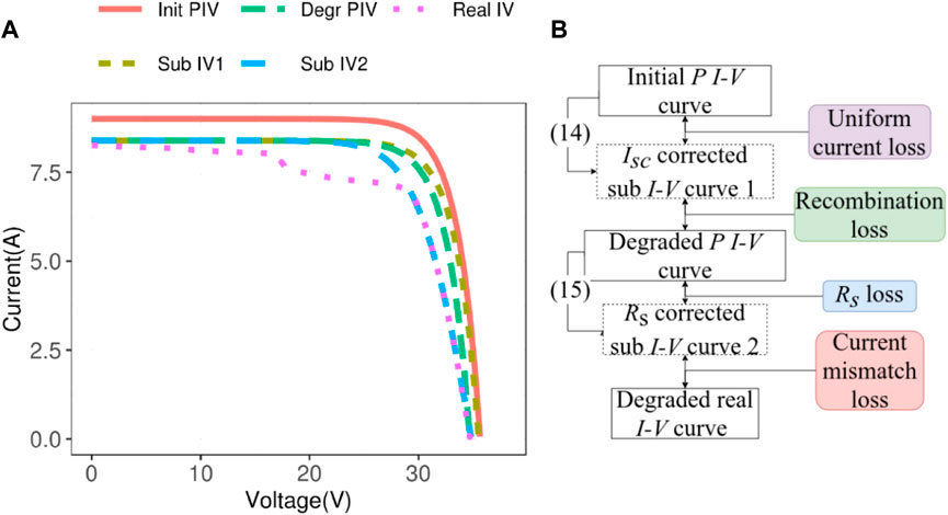
FIGURE 2. Visualization of the mechanisms extracted from the Suns-V_OC package by comparing the actual I-V curves to variations of ideal I-V curves extracted from V_OC and irradiance trends. (A) shows the overlay of the I-V curves and (B) shows the flowchart of result extraction. More detailed information can be found in Wang et al. (2020a, b). Figure is from Wang et al. (2020b).

The individual mechanisms are described as follows:

• Uniform current loss—power change due to the I_SC difference from the ideal curve

• Current mismatch—power change due to I-V curve steps created by I_SC differences between cells

• Series resistance—power change due to series resistance

• Recombination loss—power change due to a decrease in V_OC through carrier recombination

2.3.4 netSEM: network modeling of degradation pathways using Markvonian principle

The R package “netSEM v0.5.0” (Huang et al., 2018b) conducts a network statistical analysis (network structural equation modeling) on a dataframe of coincident observations of multiple continuous variables (Bruckman et al., 2013; French et al., 2015). This analysis uses Markvonian Principal and builds a pathway model by exploring a pool of domain knowledge guided by candidate statistical causal relationships between each of the variable pairs, and selecting the “best fit” on the basis of the goodness-of-fit statistic, such as the adjusted R-squared value, which measures how successful the fit is in explaining the variation of the data. The netSEM methodology is motivated by the analysis of systems that are experiencing degradation of some performance characteristic (or response) under exposure to particular stressors that are considered exogenous variables (or predictors). In addition to the direct relationship between the exogenous variables and the endogenous variable, netSEM investigates potential connections between them through other covariates. The resulting relationship diagram can be used to generate insight into the pathways of the system under observation. These pathways can be good candidates for improving the performance characteristics by identifying sequences of strong relationships that match prior domain knowledge well.

In this study, the endogenous variable is year dy, while the exogenous variables are uniform current loss uni_I, current mismatch loss I_mis, series resistance loss rs, recombination loss rec, and maximum power loss P_mp. Starting with the main endogenous variable to the last exogenous variable through the intermediate variables which are considered as exogenous variables, the nonrecursive relationships usually occur. The package outputs a flow chart style diagram, detailing the relevant characteristics of the uncovered relationships between variables. The pathway threshold cut-offs are defined by the Adj-R² values of 0.1, 0.4, and 0.7. Pathways with Adj-R² values below 0.1 are considered to have no correlation and are not connected by a line, while pathways with Adj-R² values above 0.7 are considered to have strong correlation and are connected by a thick line.

3 Results

3.1 Full-sized modules and STC I-V

3.1.1 PLR analysis

The variables used in the $<Stressor|Response>$$(<S|R>)$ are time and max power. For outdoor systems, this is best quantified as a performance loss rate (PLR), which gives the percent power loss per year of operation. It is analogous to degradation rates used to quantify PV performance, giving a directly comparable metric of performance between module types. PLR values are determined from the relationship between power and time of a system by using the PVplr R package. We are able to capture piecewise linear PLR values as well, making them an ideal use case for $<S|R>$ modeling. For clarity, PLR values that are referred to as “high” are further from zero than PLR values described as “low” in relation to the amount of power loss observed between them. For example, a PLR of −0.7%/a is referred to as higher than a PLR value of −0.3%/a, as the first value is indicative of higher power loss.

The linear and piecewise linear $<S|R>$ models are shown below in Figure 3 for each module type. The measurements have been normalized to their initial values to prevent bias from different power ratings. There is a clear changepoint trend in the Al-BSF and half-cell PERC modules, with a high initial loss followed by a more stable period. The full-cell PERC modules display a more linear trend, with the linear and piecewise linear models being more similar to each other. There are a number of highly influential outliers in some of the modules, however, which will bias the models and the location of the changepoint.

FIGURE 3

FIGURE 3. Linear and piecewise linear $<Stressor|Response>$$(<S|R>)$ of P_MP vs. time (annum) for the CSI outdoor MPPT full-sized modules. The full-sized modules were taken down for indoor I-V measurements at standard test conditions (STC) every 6 months and the data are corrected based on their initial performance. Full-szied modules of each type are grouped and modeled together.

One of the steps (step 4 for the half-cell PERC and Al-BSF modules, and step 5 for the full-cell PERC modules) showed abnormally low data. After consulting with the operators, it was found that the modules were not properly cleaned before these exposures, resulting in a large decrease in I_SC during measurement. As this change was not due to degradation within the modules and they recovered by the next step, these data were removed.

For both the half-cell PERC and Al-BSF modules, there is a sharp drop in power between the first and second measurements. This drop is captured by the piecewise linear models, which shows an initial loss of −1.70% for the Al-BSF modules and −3.45% for the half-cell PERC modules. After the initial loss period, the modules stabilize and power loss decreases.

It can be observed in Figure 3 that a number of outliers appear at a lower power than the others with the Al-BSF full-cell and particularly the full-cell PERC modules. At the final step, the PERC full-cell modules vary between 99% and 94% of initial power. Comparing the I-V curves of an example outlier (Figure 4) shows that the loss in power is primarily due to a decrease in the fill factor of the module, which suggests that this is a legitimate change in the performance of the module and not a measurement error. As the outliers appear to be legitimate losses, we do not want to remove them from analysis, and instead incorporate them into the uncertainty of our results.

FIGURE 4

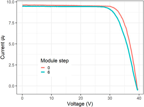
FIGURE 4. Comparison between I-V curves of a full-cell PERC full-sized module from its initial measurement (module step 0) and its final measurement (module step 6), with each step of around 6 months outdoor exposure. The final P_MP measurement of this module is an outlier compared to most of the other modules. Differences between the curves show that fill factor loss is the contributing mode of power loss.

This data trend can be directly used to evaluate the PLR for each of the module groups. For the first calculation, the data are grouped together for each module type and a single model is built for each group. These are the models shown in Figure 3. As some of the data show non-linear trends, non-linear PLR is evaluated using a single changepoint model through the PVplr package (Curran A. et al., 2020). PLR results for each segment are listed in Table 2, along with the Adj-R², changepoint, and confidence interval for each model.

TABLE 2

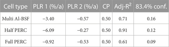
TABLE 2. Numeric PLR results of the piecewise linear models shown in Figure 3. PLR 1 indicates the first linear segment and PLR 2 refers to the second.

The Al-BSF modules showed a fitted PLR value of −3.40%/a for the first segment and −0.57%/a for the second, matching the result observed in the piecewise model fit with a trend of a high initial loss then followed by a stable period. The other module with a similar trend, PERC half-cell, showed a similar trend with higher initial PLR of −6.09%/a followed by −0.27%/a after the changepoint. The PERC full-cell modules did not show as strong a changepoint trend as the other modules, seen in both the lower adj-R² and the similar PLR values for each segment. The PLR values do follow a trend of the first being higher than the second, however, the confidence intervals overlap, so a statistically significant difference between the two PLR values is not established.

The models of the grouped modules are potentially biased by the outliers observed after 3 years of exposure. To address the outliers’ influence on the models, we fit our $<S|R>$ models again to the individual models and compared the results, instead of modeling them all together. Figure 5 shows the distribution of the piecewise linear PLR values for both the first and second segment. There are only two segments, as these are single changepoint models. The original calculations from modeling all the modules together are also shown by the diamonds to the right of each boxplot, with their 83.4% confidence intervals. Some of the confidence intervals could not be shown for the first segment, as there was only one data point available in that range if the changepoint occurs early on in the timeseries. It is observed that the values calculated by modeling the modules together trend very closely with the distributions of the individual module calculations. The half-cell PERC and Al-BSF modules show a much stronger changepoint trend given the clear difference between the first and second PLR values for each segment. Each of these modules shows a high initial loss followed by a longer period of stability. The full-cell PERC modules on the other hand show similar distributions for both segments, again due to the more linear trend. When modeling individually, the outliers are separate and more visible compared to the more regular modules.

FIGURE 5

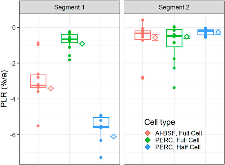
FIGURE 5. Performance loss rate (PLR) values (% per annum) for the first and second segments of the piecewise linear $<Stressor|Response>$$(<S|R>)$ for each individual full-sized module. The results of the models built from combining the modules are shown by the diamonds to the right of each boxplot.

Information about the fitting and changepoint magnitudes of the models are given in Figure 6. When modeling by individual module, the Pred-R² could not be calculated as there were only 5–6 data points, so the Adj-R² of each model is shown instead. Though there is a range of fitting by individual module, all modules show a median Adj-R² above 0.9. Again, it is made clear that the full-cell PERC modules show a very inconsistent piecewise linear trend. The changepoints are very consistently located for the Al-BSF and half-cell PERC modules, however, the full-cell PERC piecewise models fit changepoints across the time range of the system, indicating an inconsistent changepoint trend between modules.

FIGURE 6

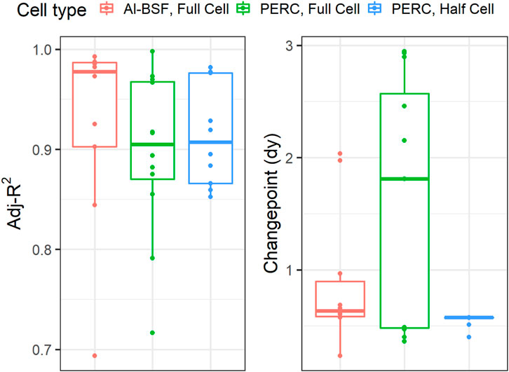
FIGURE 6. Adj-R² and changepoint magnitude for the individual $<Stressor|Response>$ ($<S|R>$) models. Pred-R² could not be calculated as there was not enough indoor I-V measurement data at standard test conditions (STC) for each field-exposed full-sized module.

3.1.2 I-V features

The Current-Voltage (I-V) features of these modules are shown below in Figure 7, colored by each of the module groups. Corresponding with an initial loss in max power, there is a drop between the first and second steps in I_SC for the half-cell PERC and Al-BSF modules, and a drop in V_OC as well for the half-cell PERC modules. The series resistance and fill factor are more stable for all module types. The changes in these features are most significant for the half-cell PERC modules, which also show the highest power drop. Given the stability of the measurements of the other modules, this is likely a feature of light induced degradation (LID) with a mixture of boron-oxygen related light induced degradation (BO-LID) and light and elevated temperature induced degradation (LeTID) occurring during the initial 6 months of exposure and saturating afterwards. The exact time frame of the LID cannot be assessed, as it occurred between the first two measurements.

FIGURE 7

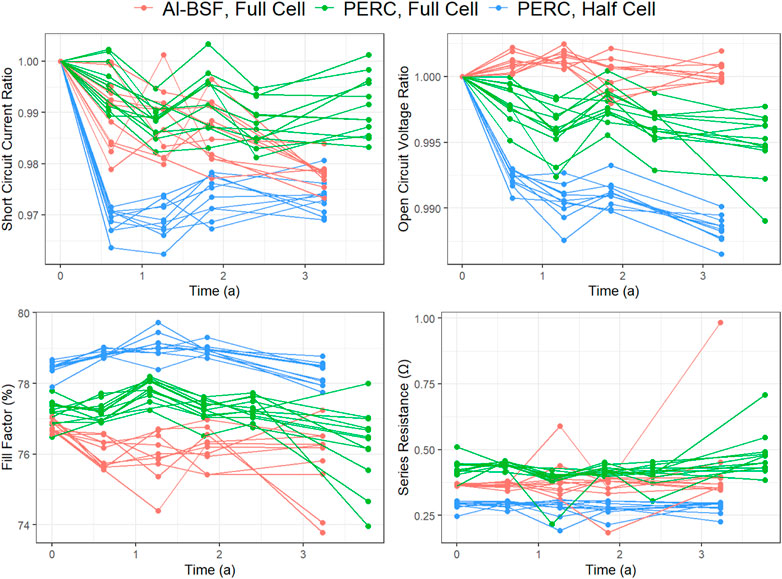
FIGURE 7. Additional I-V features changes over time (annum) of the full-sized modules colored by their cell types. Initial losses can be seen in I_SC and V_OC for the half-cell PERC modules, which correlates with an observed initial P_MP loss.

3.2 Minimodules and field I-V

3.2.1 PLR analysis

PLR values for the individual minimodules were calculated using the maximum output power (P_MP) tracking and the PVplr package. The first 30 weeks of data were excluded due to a breakdown of the load units capturing the measurements, and they had to be sent out for shipment. This led to sparse data in the beginning of the time series, which strongly influenced the modeling. As there was enough data to satisfy 2 years of exposure without this initial gap period, it was removed. Linear and piecewise linear $<S|R>$ models are represented by the linear and piecewise linear PLR values. Examples of two of the minimodules are given in Figures 8, 9 for the lowest and highest observed loss in the piecewise linear models, respectively. It is observed that in modules with high loss, such as in Figure 9, there is a strong segmented behavior with high initial losses followed by a period of stability.

FIGURE 8

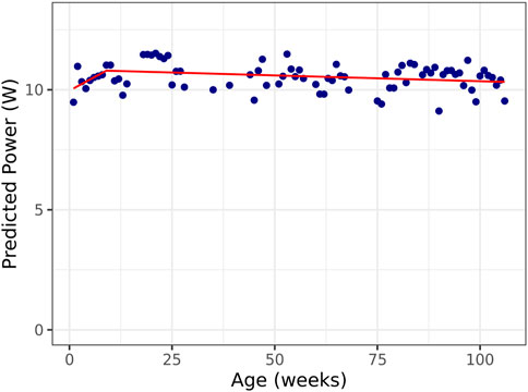
FIGURE 8. Piecewise linear performance loss rate (PLR) fit result from the field I-V data of the minimodule with the lowest loss. Minimodule variant is Al-BSF with POE/KPX encapsulant and backsheet.

FIGURE 9

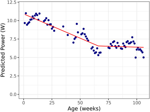
FIGURE 9. Piecewise linear performance loss rate (PLR) fit result from the field I-V data of the minimodule with the highest loss. Minimodule variant is PERC with EVA/KPX encapsulant and backsheet.

The disparities in piecewise calculated loss make more sense when we observe all of the PLR values together in Figure 10. Even among modules of the same type there can be large disparities. The PERC modules show some of the lowest values of PLR, however, this is inconsistent, with significantly different PLR being observed between modules with the same cell or packaging combinations. This would suggest that performance is highly susceptible to factors outside of packaging degradation. It is possible that soiling or differences in wiring are creating different performances between minimodules.

FIGURE 10

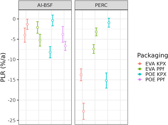
FIGURE 10. Linear performance loss rate (PLR % per annum) from the field I-V data of the outdoor CWRU minimodule. 83.4% confidence intervals are shown, indicating differences between samples to a p-value of 0.05.

3.2.2 Suns-V_OC power loss features

Suns-V_OC loss mechanisms are extracted from the I-V curve timeseries for each of the minimodules. Two examples of the resulting trend are given, from the same modules shown with the highest and lowest PLR results. Figure 11 shows the low PLR module and Figure 12 is the highest PLR module. In both cases, the recombination losses and current mismatch losses cluster strongly around zero, showing no observable trend over time. The other two mechanisms, uniform current and series resistance, show significant deviations from zero, with uniform current being positive and series resistance being negative. The series resistance loss refers to power losses due to the existence of any series resistance, so this should always be less than zero for any real module. Comparing the two modules, however, shows that the series resistance loss is much larger overall for the high PLR module (Figure 12), decreasing from near zero initially. This suggests that series resistance increases are the cause of the difference in PLR between the modules.

FIGURE 11

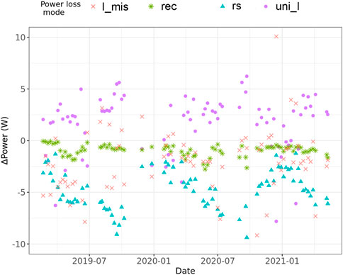
FIGURE 11. Weekly Suns-V_OC loss mechanism results for the outdoor minimodule with the lowest loss, including uniform current loss uni_I, current mismatch loss I_mis, series resistance loss rs, and recombination loss rec. Minimodule variant is Al-BSF with POE/KPX encapsulant and backsheet.

FIGURE 12

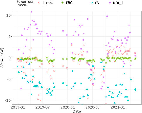
FIGURE 12. Weekly Suns-V_OC loss mechanism results for the outdoor minimodule with the highest loss, including uniform current loss uni_I, current mismatch loss I_mis, series resistance loss rs, and recombination loss rec. Minimodule variant is PERC with EVA/KPX encapsulant and backsheet.

The uniform current loss for the minimodules is unexpected, being positive. The uniform current relates to differences between the I_SC of the determined ideal curve and the actual curve, so a positive result indicates that the observed I_SC values of the I-V curves are higher than the curves at the start of the timeseries which are used to define the ‘ideal’ curve for the module. This is consistent across all of the minimodules. In outdoor timeseries the modules are assumed to be in their most ‘ideal’ operating conditions in the initial weeks of exposure, and will then go on to accumulate losses due to various degradation mechanisms over time. The initial month of data is what is used to calculate the ‘ideal’ module I_SC value that all future curves will be compared to. As such, I_SC losses in the initial operation of the modules will create an observed positive uniform current loss in the rest of the measured operation. In this specific instance, the modules needed to be re-wired with shorter and lower gauge wire shortly after installation due measurement problems caused by their lower V_OC values. This post-installation change increased the I_SC of the modules. While this is not an ideal test condition, results can still be evaluated for these modules. First, the uniform current loss is the only component that is influenced by the initial I_SC deviations; all other components are evaluated independently. Second, any I_SC trend in the performance of the modules would still be observable and quantifiable, as an initial I_SC deviation only creates a magnitude offset in the trend. This can be observed in Figures 11, 12 where sharp drops in uniform current loss can be attributed to shading instances on the minimodules.

3.2.3 netSEM modeling

netSEM modeling was applied next to build and identify the relationships between the P_MP and Suns-V_OC loss mechanisms. Again, examples are given for the two minimodules with high and low PLR values. For the models shown, the Adj-R² thresholds for the pathways were 0.1, 0.4, and 0.7. These levels control the thickness of the pathways between the variables with thicker lines indicating a better fit and no lines shown for any relationship below an Adj-R² of 0.1. The stressor and response variables are decimal years (dy) and predicted power (P_mp), respectively. The P_mp results are the same as those used in the PLR calculations, so the models show the relationships between the Suns-V_OC loss variables and the PLR of the modules.

The low PLR module (Figure 13) only shows a single pathway between measured power and time. None of the other pathways appear in the plot as they all have Adj-R² values less than 0.1. The interpretation of this is that there are no observed relationships between any of the Suns-V_OC loss mechanisms with each other, time, or power. The only trend that is observed is dy to P_mp, which is analogous to the PLR of the module. While unusual, this does match with the PLR result, which overlapped with zero. A module that is undergoing no observable degradation would not be likely to show trends between degradation features.

FIGURE 13

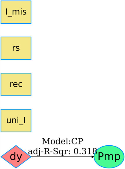
FIGURE 13. netSEM model for the low performance loss rate (PLR) minimodule. The endogenous variable is year dy, while the exogenous variables are uniform current loss uni_I, current mismatch loss I_mis, series resistance loss rs, recombination loss rec, and maximum power loss P_mp. Pathway thresholds are present at Adj-R² of 0.1, 0.4, and 0.7.

Unlike the low PLR module, the high PLR module netSEM model (Figure 14) shows much stronger paths between its variables. The strongest pathway by far is the dy to P_mp path (the PLR pathway), which shows a changepoint model with an Adj-R² of 0.921. The strong changepoint trend was also observed in the PLR analysis of the modules (Figure 9). The changepoint model is observed numerous times within the netSEM model, suggesting this trend is present in many of the mechanisms of the operation of this module. All of the other trends show fairly low Adj-R² values with the exception of a stronger trend observed between the series resistance and uniform current loss.

FIGURE 14

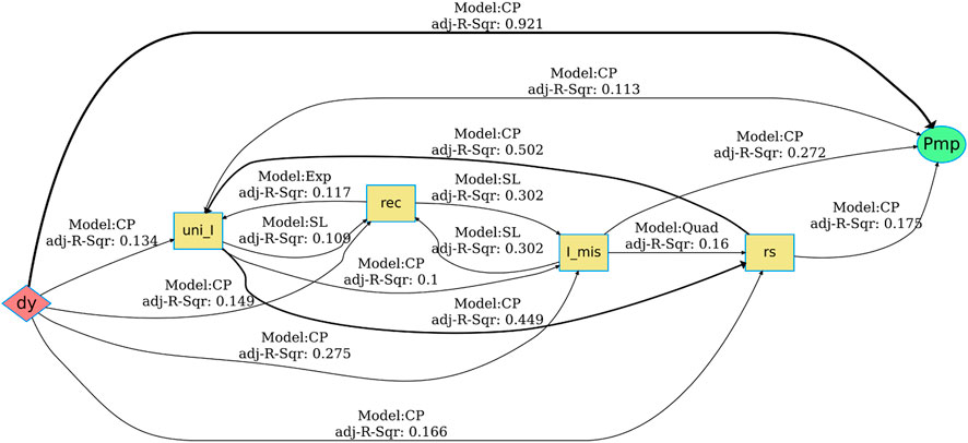
FIGURE 14. netSEM model for the high performance loss rate (PLR) minimodule. The endogenous variable is year dy, while the exogenous variables are uniform current loss uni_I, current mismatch loss I_mis, series resistance loss rs, recombination loss rec, and maximum power loss P_mp. Pathway thresholds are present at Adj-R² of 0.1, 0.4, and 0.7.

4 Discussion

4.1 Non-linear PLR: field I-V preferable to STC I-V

In this study, full-sized modules were periodically retrieved from the site every 6 months and subjected to I-V measurement in a laboratory under Standard Test Conditions (STC). Since the measurements were taken under the same conditions, the data processing is straightforward and the PLR results are presented in Figure 3.

On the other hand, minimodules were continuously monitored outdoors for field I-V measurements, which were affected by the changing irradiances and temperatures in the environment. The drawback of this technique is that it needs thousands of I-V curve measurements to build the necessary relationships between voltage and irradiance and to extract significant differences between the real and ideal curves. This is not a common way to measure modules, as it is prohibitive to power production, costs more to maintain, and generates large quantities of data that can be difficult to analyze without the proper infrastructure. Despite this, previous studies have found I-V timeseries datastreams to be tremendously important in the analysis of outdoor power performance and have had success studying them in the past Wang et al. (2020b, 2018); Liu et al. (2019) To obtain the minimodule degradation over time, we utilized the open-source data-driven tool ddiv package to correct the field I-V data to the reference condition, and the results are shown in Figures 8, 9. In some cases, particularly for minimodules with high degradation, such as in Figure 9, we observed a segmented behavior with high initial losses followed by a period of reduced loss, i.e., non-linear PLR (Lindig et al., 2022; Livera et al., 2022b; Curran A. J. et al., 2020).

Comparing the low temporal resolution STC I-V to the continuous high-resolution field I-V, it is more challenging to accurately identify the changepoint and the underlying degradation mechanism being studied for the STC I-V method. Hence, we believe that continuous field I-V measurements are preferable over STC I-V for PV PLR analysis.

4.2 Field PLR: full-sized module preferable to minimodule

Overall, we find PLR of full-sized modules lower and more consistant compared to minimodules. Minimodule studies showed inconsistent performance due to significant power loss contributions via series resistance, likely from the wiring between the load unit and the minimodules (Yu et al., 2023), contributing to high power loss.

4.2.1 Performance loss

The performance losses of full-sized modules were quite low and consistent, as shown in Figure 3. There were distributions of performance within each module group, however, the results from the combined models were similar to the mean and median of the individual modules. This shows that the observed trends in the modules, namely, the changepoint behavior in the half-cell PERC and Al-BSF, occurred consistently across all of the 10–12 modules in each group.

Unlike the exposure of full-sized modules, the minimodules showed both higher PLR values than expected for fielded modules and did not cluster by module type. There are only a few instances of modules with the same cell and packaging combinations showing overlapping PLR results. It is observed that PERC cells tended to have higher PLR values with the three highest results being PERC cells, however, the extreme nature of the results suggest influences beyond degradation. PLR values of −5%/a over 2 years would be nearly an order of magnitude greater than expected for commercial modules and it is unlikely that outdoor degradation alone would create such power loss results.

4.2.2 Degradation mechanism

For full-sized modules, there is a clear initial power loss for the half-cell PERC and Al-BSF modules, more significantly for the half-cell PERC module. This was observed both in the power (Figure 3) and in the I_SC (Figure 7) of the modules, with the half-cell PERC showing an additional loss in V_OC initially (Figure 7). This is typical behavior of boron-oxygen related light induced degradation (BO-LID), which is expected to be observed more in PERC modules. The BO-LID effects were not observed in the full-cell PERC modules, however, these full-sized modules were from a separate exposure and it is possible they were preconditioned or any BO-LID effects had already saturated by the time the first measurements were taken.

In comparison to full-sized modules, we observed significant variation in the degradation mechanism of minimodules, both between different cell/packaging variants and even within the same module variant. While the PLR results themselves are not very diagnostic, the Suns-V_OC results in Figures 11, 12, and similarly all the remaining results in the Supplementary Material, give additional insight into the performance of the minimodules. In all cases, the current mismatch and recombination values are stable at zero and show little to no relationship to time of power in the netSEM models. Recombination loss is evaluated from decreases in the open-circuit voltage and is certainly something that would appear under cases of LID, as was observed in the half-cell PERC full-sized modules. Comparing the extremes of the PLR results shows a significant difference in the amount of loss due to series resistance, which suggests that the modules experiencing high PLR have much higher series resistance than the lower PLR modules. While degradation mechanisms such as metallization corrosion (Iqbal et al., 2022) can induce series resistance increases, the high degree of power loss suggests that the problems are external of the modules. As minimodules have much lower voltage than full-sized modules, they are more susceptible to the PV connectors and wiring between them and the I-V tracer. It is possible that the observed losses in series resistance are due to changes in the resistance between the load unit and the modules, which would explain why there do not appear to be strong trends between the types of modules. Despite the potential influence from the connections, there are still conclusions that can be made from the modules. The Suns-V_OC results show clearly that the V_OC of the modules are highly stable, and it is unlikely that any recombination increase has occurred during the outdoor period.

The example netSEM models, such as Figures 13, 14, and similarly all the remaining results in the Supplementary Material, show a clear pattern of signal or lack of signal in the performance of the modules. Degradation or performance change can be thought of as a signal over time in the measurements of a module. In a perfect module, one would not expect any internal changes and as such there would be no available signal to model and quantify. Such is the case in the low PLR module. The PLR value for this module is less than zero, but its confidence interval overlaps with zero, so it cannot be stated that any loss at all has occurred in its power production. As such, the netSEM model between the power, time, and Suns-V_OC features shows little signal, with only the trend between time and power having an Adj-R² above the low threshold of 0.1. Conversely, the high PLR module shows much stronger pathways, particularly between power and time. That the improved pathway fits is an indication that there is observable degradation over time occurring within the high PLR module. There is a consistent trend in the netSEM models where the uniform current and the series resistance show strong paths with each other. The other Suns-V_OC loss mechanisms, recombination and current mismatch, show weaker trends between the other variables, which is expected because they are stable over time. This implies that there is a correlation between the series resistance and the offset between ideal and measured I_SC (Asadpour et al., 2019). Since we observed inconsistency between the modules and there is an extreme R_S loss in some module variants, we believe that the issue should mainly be related to the connectors and wiring between the load unit and minimodules.

4.3 Comparable reliability: PERC vs. Al-BSF

Due to the inconsistency performance among minimodules, we use only results of full-sized modules to compare the reliability of PERC and Al-BSF. Piecewise PLR was able to quantify the initial losses, −6.09%/a for half-cell PERC and −3.40%/a for Al-BSF, however, this trend occurred between low temporal resolution measurements. The LID losses occurred between the first and second I-V measurements, which were taken roughly 6 months apart. As only the start and end of this change was captured, it is unknown at what point in this 6-month period the drop and saturation occurred. From a PLR standpoint, the same loss in power over a shorter period of time would lead to a more negative PLR result. It is possible that the actual PLR quantification of the LID would be more negative than what was calculated, however, more measurements would have to have been taken at the start of the exposure to capture this.

As is expected, the LID effects quickly saturated and the modules resumed more stable trends. The PLR results after the LID saturation is a better indicator of long term performance, so these are used when discussing overall performance of the module. The half-cell PERC modules were the best performers, having a PLR value of −0.27% ± 0.12%/a, closest to zero.

The full-cell PERC and Al-BSF modules showed PLR values of −0.53% ± 0.09%/a and −0.57% ± 0.16%/a, respectively. Although the Al-BSF modules exhibited a lower PLR compared to the full-cell PERC modules, their confidence intervals overlapped, suggesting that no statistically significant difference in their performance was observed. Overall, the PLR values were quite low and well within the expected results for commercial modules and consistent with what has been reported (Theristis et al., 2023; Jordan et al., 2022).

5 Conclusion

A series of outdoor exposures were performed with the intent of observing the performance PERC and Al-BSF modules in a realistic operating environment. The study was split into two exposures. One with full-sized modules was exposed outdoors and taken down periodically for indoor I-V measurements. The other was an exposure of 4 cell minimodules with timeseries minute interval max power and 10-min interval I-V tracking. Results from the full-sized module study shows initial losses attributed to LID, most significantly in half-cell PERC modules, but not in full-cell PERC modules, which may have already saturated any LID effects. Performance loss rate calculation showed significant changepoint behavior due to LID effects in half-cell PERC and Al-BSF modules. Once LID had saturated, the half-cell PERC modules showed the best performance with a PLR value of −0.27% ± 0.12%/a. The full-cell PERC and Al-BSF modules showed PLR values of −0.53% ± 0.09%/a and −0.57% ± 0.16%/a, respectively, which have overlapping confidence intervals and are therefore not statistically significant.

The minimodule study showed highly variable PLR results, which did not group by module type. Suns-V_OC analysis showed a strong influence of series resistance, likely from the wiring between the load unit and the minimodules, contributing to high power loss. Despite this, it was observed that recombination loss did not occur within the modules, suggesting resistance to LID degradation. Network structural equation models show better correlation between mechanistic variables in modules with high PLR results, indicating mechanistic change.

Data availability statement

The raw data supporting the conclusion of this article will be made available by the authors, without undue reservation.

Author contributions

JB, LB, and RF oversaw and led the research. AC, LB, JB, and RF contributed to conception and design of the study. AC, JL, XY, and J-NJ collected the data and organized the database. AC and JL performed the statistical analysis and created fit models. BB and J-NJ provided materials and samples. AC, XY, JB, LB, and RF wrote sections of the manuscript. All authors contributed to the article and approved the submitted version.

Funding

This material is based upon work supported by the U.S. Department of Energy’s Office of Energy Efficiency and Renewable Energy (EERE) under Solar Energy Technologies Office (SETO) Agreement Number DE-EE-0008172.

Acknowledgments

This work made use of the High Performance Computing Resource in the Core Facility for Advanced Research Computing at Case Western Reserve University.

Conflict of interest

Author BB was employed by Cybrid Technologies Inc. Author J-NJ was employed by CSI Solar Co. Ltd.

The remaining authors declare that the research was conducted in the absence of any commercial or financial relationships that could be construed as a potential conflict of interest.

Publisher’s note

All claims expressed in this article are solely those of the authors and do not necessarily represent those of their affiliated organizations, or those of the publisher, the editors and the reviewers. Any product that may be evaluated in this article, or claim that may be made by its manufacturer, is not guaranteed or endorsed by the publisher.

Supplementary material

The Supplementary Material for this article can be found online at: https://www.frontiersin.org/articles/10.3389/fenrg.2023.1127775/full#supplementary-material

References

Asadpour, R., Sun, X., and Alam, M. A. (2019). Electrical signatures of corrosion and solder bond failure in c-Si solar cells and modules. IEEE J. Photovoltaics9, 759–767. doi:10.1109/JPHOTOV.2019.2896898

CrossRef Full Text | Google Scholar

Braid, J. L., Curran, A. J., Sun, J., Schneller, E. J., Fada, J. S., Liu, J., et al. (2018). “El and i-v correlation for degradation of perc vs. al-bsf commercial modules in accelerated exposures,” in 2017 IEEE 44th Photovoltaic Specialist Conference (PVSC), 1261–1266. doi:10.1109/PVSC.2018.8547420

CrossRef Full Text | Google Scholar

Bruckman, L. S., Wheeler, N. R., Ma, J., Wang, E., Wang, C. K., Chou, I., et al. (2013). Statistical and domain analytics applied to PV module lifetime and degradation science. IEEE Access1, 384–403. doi:10.1109/ACCESS.2013.2267611

CrossRef Full Text | Google Scholar

Curran, A., Burleyson, T., Lindig, S., Moser, D., and French, R. (2020a). PVplr: Performance loss rate analysis pipeline. R. package version

Curran, A. J., Burleyson, T. L., Rath, K., Xin, A. S., Lindig, S., Moser, D., et al. (2020b). “Pvplr: R package implementation of multiple filters and algorithms for time-series performance loss rate analysis,” in 2020 47th IEEE Photovoltaic Specialists Conference (PVSC) (IEEE), 2086–2090. doi:10.1109/PVSC45281.2020.9300807

CrossRef Full Text | Google Scholar

Deline, C. A., Ayala Pelaez, S., Marion, W. F., Sekulic, W. R., Woodhouse, M. A., and Stein, J. (2019). Bifacial PV system performance: Separating fact from fiction. In Tech. rep. Golden, CO (United States), Chicago IL: National Renewable Energy Lab NREL

Google Scholar

Ding, S., Yang, C., Qin, C., Ai, B., Sun, X., Yang, J., et al. (2022). Comparison of LID and electrical injection regeneration of PERC and Al-bsf solar cells from a cz-Si ingot. Energies15, 7764. doi:10.3390/en15207764

CrossRef Full Text | Google Scholar

Fokuhl, E., Naeem, T., Schmid, A., Gebhardt, P., Geipel, T., and Philipp, D. (2019). “Letid—A comparison of test methods on module level,” in 36th European PV Solar Energy Conference and Exhibition, 816–821.36

Google Scholar

Fokuhl, E., Philipp, D., Mülhöfer, G., and Gebhardt, P. (2021). LID and LETID evolution of PV modules during outdoor operation and indoor tests. EPJ Photovoltaics12, 9. doi:10.1051/epjpv/2021009

CrossRef Full Text | Google Scholar

French, R. H., Bruckman, L. S., Moser, D., Lindig, S., van Iseghem, M., Müller, B., et al. (2021). “Assessment of performance loss rate of PV power systems,” in Assessment of performance loss rate of PV power systems (Geneva, Switzerland: IEA-PVPS). T13-22:2021 in IEA-PVPS 78.

Google Scholar

French, R. H., Podgornik, R., Peshek, T. J., Bruckman, L. S., Xu, Y., Wheeler, N. R., et al. (2015). Degradation science: Mesoscopic evolution and temporal analytics of photovoltaic energy materials. Curr. Opin. Solid State Mater. Sci.19, 212–226. doi:10.1016/j.cossms.2014.12.008

CrossRef Full Text | Google Scholar

Hashemi, B., Cretu, A.-M., and Taheri, S. (2020). Snow loss prediction for photovoltaic farms using computational intelligence techniques. IEEE J. Photovoltaics10, 1044–1052. doi:10.1109/JPHOTOV.2020.2987158

CrossRef Full Text | Google Scholar

Hashemi, B., Taheri, S., Cretu, A.-M., and Pouresmaeil, E. (2021). Systematic photovoltaic system power losses calculation and modeling using computational intelligence techniques. Appl. Energy284, 116396. doi:10.1016/j.apenergy.2020.116396

CrossRef Full Text | Google Scholar

Huang, W.-H., Ma, X., and French, R. H. (2018a). ddiv: Data driven I-v feature extraction. R package version 0.1.0.

Google Scholar

Huang, W.-H., Wheeler, N., Klinke, A., Xu, Y., Du, W., Verma, A. K., et al. (2018b). netSEM: Network structural equation modeling. R package version 0.5.1.

Google Scholar

Ino, Y., Heito, S., Itou, N., Niira, K., Shirasawa, K., and Takato, H. (2023). Investigation of light-induced degradation in B-doped mono-like silicon PERC cells by a cycling test with light soaking and dark annealing. IEEE J. Photovoltaics13, 48–55. doi:10.1109/JPHOTOV.2022.3229484

CrossRef Full Text | Google Scholar

Iqbal, N., Colvin, D. J., Schneller, E. J., Sakthivel, T. S., Ristau, R., Huey, B. D., et al. (2022). Characterization of front contact degradation in monocrystalline and multicrystalline silicon photovoltaic modules following damp heat exposure. Sol. Energy Mater. Sol. Cells235, 111468. doi:10.1016/j.solmat.2021.111468

CrossRef Full Text | Google Scholar

Jain, P., Poon, J., Singh, J. P., Spanos, C., Sanders, S. R., and Panda, S. K. (2020). A digital twin approach for fault diagnosis in distributed photovoltaic systems. IEEE Trans. Power Electron.35, 940–956. doi:10.1109/TPEL.2019.2911594

CrossRef Full Text | Google Scholar

Jordan, D. C., Anderson, K., Perry, K., Muller, M., Deceglie, M., White, R., et al. (2022). Photovoltaic fleet degradation insights. Prog. Photovoltaics Res. Appl.30, 1166–1175. doi:10.1002/pip.3566

CrossRef Full Text | Google Scholar

Jordan, D. C., Kurtz, S. R., VanSant, K., and Newmiller, J. (2016). Compendium of photovoltaic degradation rates. Prog. Photovoltaics Res. Appl.24, 978–989. doi:10.1002/pip.2744

CrossRef Full Text | Google Scholar

Karas, J., Repins, I., Berger, K. A., Kubicek, B., Jiang, F., Zhang, D., et al. (2023). “Results from an international interlaboratory study on light- and elevated temperature-induced degradation (LETID) in solar modules,” in Tech. Rep. NREL/PR-5K00-82118 (Golden, CO (United States): National Renewable Energy Lab. NREL).

Google Scholar

Kashyap, S., Madan, J., and Pandey, R. (2022a). Design and parametric optimization of ion-implanted PERC solar cells to achieve 22.8% efficiency: A process and device simulation study. Sustain. Energy & Fuels6, 3249–3262. doi:10.1039/D2SE00434H

CrossRef Full Text | Google Scholar

Kashyap, S., Madan, J., Pandey, R., and Ramanujam, J. (2022b). 22.8% efficient ion implanted PERC solar cell with a roadmap to achieve 23.5% efficiency: A process and device simulation study. Opt. Mater.128, 112399. doi:10.1016/j.optmat.2022.112399

CrossRef Full Text | Google Scholar

Kashyap, S., Pandey, R., Madan, J., and Sharma, R. (2022c). Design and simulations of 24.7% efficient silicide on oxide-based electrostatically doped (SILO-ED) carrier selective contact PERC solar cell. Micro Nanostructures165, 207200. doi:10.1016/j.micrna.2022.207200

CrossRef Full Text | Google Scholar

Kashyap, S., Pandey, R., Madan, J., and Sharma, R. (2022d). “Silicide on oxide based carrier selective front contact for 24% efficient PERC solar cell,” in 2022 IEEE VLSI Device Circuit and System (VLSI DCS), 234–237. doi:10.1109/VLSIDCS53788.2022.9811447

CrossRef Full Text | Google Scholar

Kashyap, S., Shrivastav, N., Pandey, R., Madan, J., and Sharma, R. (2022e). Double polo carrier selective contact based PERC solar cell for 25.5% conversion efficiency: A simulation study. ECS Trans.107, 6365–6370. doi:10.1149/10701.6365ecst

CrossRef Full Text | Google Scholar

Kersten, F., Engelhart, P., Ploigt, H.-C., Stekolnikov, A., Lindner, T., Stenzel, F., et al. (2015). “A new mc-si degradation effect called letid,” in 2015 IEEE 42nd Photovoltaic Specialist Conference (PVSC) (IEEE), 1–5. doi:10.1109/PVSC.2015.7355684

CrossRef Full Text | Google Scholar

Krauss, K., Fertig, F., Menzel, D., and Rein, S. (2015). Light-induced degradation of silicon solar cells with aluminiumoxide passivated rear side. Energy Procedia77, 599–606. doi:10.1016/j.egypro.2015.07.086

CrossRef Full Text | Google Scholar

Li, B., Karin, T., Meyers, B. E., Chen, X., Jordan, D. C., Hansen, C. W., et al. (2023). Determining circuit model parameters from operation data for PV system degradation analysis: Pvpro. Sol. Energy254, 168–181. doi:10.1016/j.solener.2023.03.011

CrossRef Full Text | Google Scholar

Lindig, S., Theristis, M., and Moser, D. (2022). Best practices for photovoltaic performance loss rate calculations. Prog. Energy4, 022003. doi:10.1088/2516-1083/ac655f

CrossRef Full Text | Google Scholar

Lindroos, J., and Savin, H. (2016). Review of light-induced degradation in crystalline silicon solar cells. Sol. Energy Mater. Sol. Cells147, 115–126. doi:10.1016/j.solmat.2015.11.047

CrossRef Full Text | Google Scholar

Liu, J., Wang, M., Curran, A. J., Maroof Karimi, A., Huang, W.-h., Schnabel, E., et al. (2019). “Real-world PV module degradation across climate zones determined from suns-voc, loss factors and I-V steps analysis of eight years of I-V, Pmp time-series datastreams,” in 2019 IEEE 46th Photovoltaic Specialists Conference (PVSC), 0680–0686. doi:10.1109/PVSC40753.2019.8980541

CrossRef Full Text | Google Scholar

Livera, A., Theristis, M., Makrides, G., and Georghiou, G. E. (2019). Recent advances in failure diagnosis techniques based on performance data analysis for grid-connected photovoltaic systems. Renew. Energy133, 126–143. doi:10.1016/j.renene.2018.09.101

CrossRef Full Text | Google Scholar

Livera, A., Theristis, M., Micheli, L., Stein, J. S., and Georghiou, G. E. (2022a). Failure diagnosis and trend-based performance losses routines for the detection and classification of incidents in large-scale photovoltaic systems. Prog. Photovoltaics Res. Appl.30, 921–937. doi:10.1002/pip.3578

CrossRef Full Text | Google Scholar

Livera, A., Tziolis, G., Theristis, M., Stein, J. S., and Georghiou, G. E. (2022b). “Performance loss rate estimation of fielded photovoltaic systems based on statistical change-point techniques,” in 2022 2nd International Conference on Energy Transition in the Mediterranean Area (Thessaloniki, Greece: SyNERGY MED), 1–6. doi:10.1109/SyNERGYMED55767.2022.9941390

CrossRef Full Text | Google Scholar

López-Escalante, M., Fernández-Rodríguez, M., Caballero, L., Martín, F., Gabás, M., and Ramos-Barrado, J. (2018). Novel encapsulant architecture on the road to photovoltaic module power output increase. Appl. Energy228, 1901–1910. doi:10.1016/j.apenergy.2018.07.073

CrossRef Full Text | Google Scholar

Meena, R., Kumar, M., and Gupta, R. (2022). Investigation of dominant degradation mode in field-aged photovoltaic modules using novel differential current-voltage analysis approach. Prog. Photovoltaics Res. Appl.30, 1312–1324. doi:10.1002/pip.3580

CrossRef Full Text | Google Scholar

Nalin Venkat, S., Yu, X., Liu, J., Wegmueller, J., Jimenez, J. C., Barcelos, E. I., et al. (2023). Statistical analysis and degradation pathway modeling of photovoltaic minimodules with varied packaging strategies. Front. Energy Res.11. doi:10.3389/fenrg.2023.1127796

CrossRef Full Text | Google Scholar

Philipps, S. (2023). Photovoltaics report. Tech. Rep., fraunhofer institute for solar energy systems, ISE. Freiburg, German.

Google Scholar

R Core Team (2020). R: A language and environment for statistical computing. Vienna, Austria: R Foundation for Statistical Computing.

Google Scholar

Sinton, R. A., and Cuevas, A. (2000). “A quasi-steady-state open-circuit voltage method for solar cell characterization,” in 16th European Photovoltaic Solar Energy Conference, Glasgow, UK, 1–4.

Google Scholar

Theristis, M., Livera, A., Micheli, L., Ascencio-Vásquez, J., Makrides, G., Georghiou, G. E., et al. (2021). Comparative analysis of change-point techniques for nonlinear photovoltaic performance degradation rate estimations. IEEE J. Photovoltaics11, 1511–1518. doi:10.1109/JPHOTOV.2021.3112037

CrossRef Full Text | Google Scholar

Theristis, M., Stein, J. S., Deline, C., Jordan, D., Robinson, C., Sekulic, W., et al. (2023). Onymous early-life performance degradation analysis of recent photovoltaic module technologies. Prog. Photovoltaics Res. Appl.31, 149–160. doi:10.1002/pip.3615

CrossRef Full Text | Google Scholar

Trube, J. (2022). International technology roadmap for photovoltaic 2022. Tech. Rep. ITRPV-VDMA.

Google Scholar

Wang, M., Burleyson, T. J., Liu, J., Curran, A. J., Gok, A., Schneller, E. J., et al. (2020a). SunsVoc: Constructing suns-voc from outdoor time-series I-V curves. R package version 0.1.1.

Google Scholar

Wang, M., Curran, A. J., Schneller, E. J., Dai, J., Pradhan, A., Qin, S., et al. (2019). “Degradation of PERC and Al-bsf photovoltaic cells with differentiated mini-module packaging under damp heat exposure,” in 2019 IEEE 46th Photovoltaic Specialists Conference (PVSC), Chicago, IL, USA (IEEE), 1–7. doi:10.1109/PVSC40753.2019.9198980

CrossRef Full Text | Google Scholar

Wang, M., Liu, J., Burleyson, T. J., Schneller, E. J., Davis, K. O., French, R. H., et al. (2020b). Analytic Isc–Voc method and power loss modes from outdoor time-series I–V curves. IEEE J. Photovoltaics10, 1379–1388. doi:10.1109/JPHOTOV.2020.2993100

CrossRef Full Text | Google Scholar

Wang, M., Ma, X., Huang, W., Liu, J., Curran, A. J., Schnabel, E., et al. (2018). Evaluation of photovoltaic module performance using novel data-driven i-v feature extraction and suns-voc determined from outdoor time-series i-v curves. In 2018 IEEE 7th World Conference on Photovoltaic Energy Conversion (WCPEC) (A Joint Conference of 45th IEEE PVSC, 28th PVSEC 34th EU PVSEC). 0778–0783. doi:10.1109/PVSC.2018.8547772

CrossRef Full Text | Google Scholar

Yu, X., Huang, B., Lv, R., Jaubert, J.-N., Xu, T., and Zhang, G. (2023). “Pv connectors, bottleneck of 40 years lifetime modules?,” in PV reliability workshop (Lakewood, Colorado, 1–5.

Google Scholar