 Zhijian Guo
 Jian Yu
95% of researchers rate our articles as excellent or good
Learn more about the work of our research integrity team to safeguard the quality of each article we publish.
Find out more
ORIGINAL RESEARCH article
Front. Energy Res. , 22 March 2023
Sec. Process and Energy Systems Engineering
Volume 11 - 2023 | https://doi.org/10.3389/fenrg.2023.1123548
This article is part of the Research Topic Advanced Technologies of Integrated Energy System for Carbon Neutrality View all 7 articles
Recently, in order to reduce carbon emissions and meet climate change targets set by governments worldwide, which has led to the growth of renewable energy sources, such as wind, solar and hydropower energy, more and more ± 800 kV power lines have been built for more than 1500 km long-distance transmission, and the total and ionized field under it serve as important assessment indicators of an electromagnetic field. To calculate the total electric field and ionized field under UHVDC power lines, based on the upwind difference idea proposed by Takuma, the boundary condition and initial value selection are improved with the Kaptzov hypothesis as the boundary condition, and the difference between the surface field strength on the wire and the critical coronal voltage is used as the benchmark to estimate the initial value of charge density. By adopting the improved method, the calculation results of the total electric field and ionized field under the ± 800 kV power lines in typical high altitude regions suggest that the total electric field on the ground increases with the decrease in the wire’s height above ground, while the ion current density goes up with the reduction in the roughness coefficient of the wire; when the ± 800 kV power lines stipulated by national standards go through the residential areas, and the wire’s minimum height above ground is 21 m, total electric field and ionized field under the power lines are less than the limits set by national standards. Also, the calculation method proposed in this paper is suitable for the calculation of ground total electric field for future ± 1,200 kV power lines, which can provide reference for UHVDC power line designing and carbon emission target realization.
Ultra-high-voltage power lines play a significant role in transmitting long-distance and large-capacity electrical energy, as well as one of the major methods to solve the imbalanced distribution between energy sources and energy consumption sites (Liu, 2009a; Liu, 2009b). On this basis, multiple ± 800 kV power lines have been successively built in China in recent years. However, along with the increase of the voltage level, the electric field on the surface of these lines also enhances constantly, easily leading to corona discharge and generating corresponding space charge. The total electric field is a product of the electric field generated by space charge and the standard electric field from wire pressurization (Zhao, 2004). In UHVDC transmission projects, the total electric field occupies a key role in the electromagnetic environment of UHVDC transmission projects, as well as in the circuit design.
To analyze electromagnetic environment issues of UHVDC lines, scholars in China and other countries have conducted lots of experimental studies (HIRSCH and SCHAFER, 1969; MARUVADA et al., 1981a; MARUVADA et al., 1981b; FU, 1993; Min et al., 2011). However, as these experiments only focused on experimental lines with typical parameters and voltage levels in a specific environment, their application scope is subject to limitations. As a result, certain simulation methods must be adopted for predicting and calculating the total and ionized field of UHVDC lines. The calculation methods for UHVDC ion current are generally classified into two categories: the Deutsch hypothesis-based flux-tracing method, and the meshing-based numerical method.
In 1969, Maruvada and Janischewskyj (SARMA and JANISCHEWSKYJ, 1969a; SARMA and JANISCHEWSKYJ, 1969b) introduced the Deutsch hypothesis to accelerate the speed of solving equations. They believed that since the space charge does not change the direction of electric field lines, a nominal field could be calculated first, and then iterations are made on the nominal electric field to solve electric potential and charge density, further simplifying the question into a one-dimensional one. Later, Sunaga (SUNAGA and SAWADA, 1980) et al. made some improvements to the boundary condition of the flux line method for analyzing the influence of space charge on radio interference. Yet, total electric field lines may severely deviate from nominal electric field lines because the introduction of the Deutsch hypothesis will lead to great error and the impact of wind velocity cannot be neglected. Moreover, the calculation accuracy may decrease in the case of a complex line structure. Therefore, along with the increased computer capacity, more researchers began to abandon the Deutsch hypothesis but resorted to two-dimensional models for solving the direct-current ionized field.
The Canadian scholar Janischewckj (JANISCHEWSKYJ and CELA, 1979) innovatively adopted the FEM for calculating direct-current ionized field: the charge density in the space is predetermined as the initial value, and then differential equations are adopted for calculations; if the calculated results deviate from the initial value, the original initial value will be modified for repeated calculations and iterations until they become consistent. Nevertheless, as the charge density equations belong to strong convection equations, and iterative solving will easily bring about numerical oscillation, the Japanese scholar Takuma and Wang (TAKUMA et al., 1982; WANG et al., 2018; WANG et al., 2019) introduced the upwind difference to the solving process for improvement. Still, the upwind finite element method relies on experimental measurements when selecting boundary conditions of ion transport equations, so the application scope of this method is restricted.
Based on the above analyses, the method of computed the total electric field and ionized field on the ground proposed here is built upon Takuma’s upwind difference method but with improved boundary conditions and initial values. After that, the proposed calculation method is employed for exploring the distribution rules of total electric field and ionized field on the ground under different cross arm height of typical ±800 kV power lines in the high-altitude regions, thus verifying whether the total electric field and ionized field on the ground meet the limits set by national standards by using the current wire models of typical ± 800 kV power lines.
When the surface field strength of DC power lines is greater than the starting corona strength, the air around the surface of the lines will ionize, and space charges generated by ionization will move along the direction of the lines. With the bipolar direct-current lines as an example, the entire space can be roughly divided into three regions as indicated in Figure 1, where the area from positive wires to the Earth is filled with kations, while area from negative wires to the Earth is full of anions, with positive and negative ions coexisting wthin the space of two wires. These space charges will cause a unique effect on the direct-current transmission lines. Space charges themselves will generate an electric field, which greatly enhances the electric field produced by wire charges; meanwhile, space charges will move under the electric field action and form an ion current. Ion current is determined by the voltage and the field generated by ions, but the relationship is non-linear.
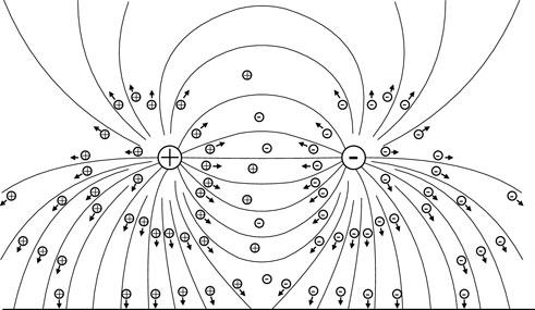
FIGURE 1. Schematic diagram of the ionized field of bipolar direct-current transmission lines.
The following premises are adopted for simplicity.
A) All parameters are time-invariant 2-D (only have tow components on the cross-sections of the lines); only uniform corona discharge is considered mainly because real transmission lines are arranged in parallel. Thus, it is assumed that a two-dimensional problem of the corona field is solved on the premise of neglecting poles and towers, conductor sag, and wire end effect.
B) Compared with the drift, the ion diffusion effect is very small and can be neglected; due to low ion concentration (generally nC/m3), the diffusion effect caused by concentration difference is quite small, so only the drift is considered.
C) Mobility of kations and anions is a constant irrelevant to the field strength, and ion mobility only depends on the charge-mass ratio, which is an inherent attribute of ions but irrelevant to the field strength; if the simplified ion mobility is adopted, it is correlated with the field strength.
D) The thickness of the ionic layer can be neglected; the ionized layer generally has a thickness of about mm-grade, which can be neglected compared to the wire height above ground of a few dozen meters.
For the bipolar direct-current ionized field, the equations to be solved include:
Poisson Equation:
Ion Current Equation:
Current Continuity Equation:
Calculation processes are shown in Figure 2. First, assumming the charge density on boundary points is constant; then, the electric field and density of space charge are iteratively solved until the steady-state solution under the boundary condition of this charge density is obtained; finally, based on Kaptzov hypothesis, the assumed boundary condition of the surface charge density on the wire are modified, and the space charge density spreading is calculated repeatedly until Kaptzov hypothesis is met.
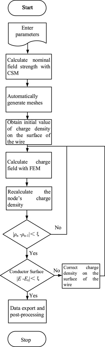
FIGURE 2. Flow chart for the calculation of DC corona field on power lines.
The electric potential’s boundary condition is expressed as follows.
On the ground and on the Earth wire:
On the transmission lines:
To determine the ionized field, the boundary condition of the electric field or electric charge shall also be in place. According to Takuma, supposing that the constant surface charge density on the wire is used as the boundary conditions of the charge, then we get the following equations.
Near the positive wire:
Near the negative wire:
In this way, electric charges on the surface of the wire shall be deduced through experiments or empirical formulas before calculations are made, thus reducing the accessibility or reliability of the calculations.
In this study, the field strength remains unchanged at the corona field strength on the surface of the wire.
Near the positive wire:
Near the negative wire:
where
The initial corona field strength of AC lines is calculated by Peek via a great number of experiments. If it is believed that corona onset field of both DC and AC power lines have the same peaks, so Peek’s formula can be transformed into the following DC form.
where
Eq. 12 presents the results under standard atmospheric pressure. In the case of high-altitude areas with lower atmospheric pressure, the correction coefficient of the atmosphere shall be considered, namely,
There are three independent unknown variables in the bipolar direct-current ionized field. Here,
To calculate the ionized field, by adopting the boundary condition, Poisson Equation and the above two equations are adopted for computing the unknown variables, namely, potential, and space charge density. Iterative solving can be used for the calculation. First, the charge density distribution is fixed, a space-based electric field under certain charge density distribution is obtained and the charge density is calculated. This process is repeated until the field and charge density distribution reach a stable state, as shown in Figure 3.
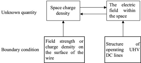
FIGURE 3. Iterative solving process of DC ionized field.
When solving the electric potential
where
In terms of nominal field, multiple images or charge simulation methods are generally adopted for rapidly and accurately solving Poisson Equation. In this study, finite element meshes are divided into triangles, and the same unit partition is also applied to the subsequent charge solving process.
To solve the electric charge, the gradient of node potential shall be obtained, namely
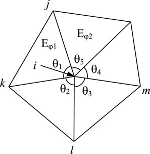
FIGURE 4. Schematic diagram of electric field interpolation distributed based on angles.
To avoid numerical oscillation, upwind discrete equations are adopted while differentially solving the charge density equations. Physically, it can be considered that charge density flows under the electric field effect, and the value at a certain point
Taking Figure 5 as an example,
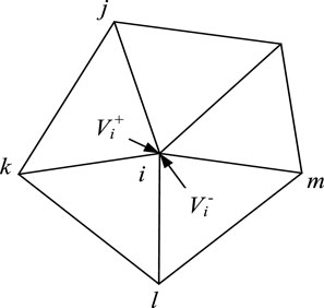
FIGURE 5. Schematic diagram of upwind difference.
The coordinates and potentials of the three points are written into:
The difference shape function within the unit can be expressed as:
Thus, the potential gradient is obtained:
Supposing that
The calculation equation of positive charges within the unit
Finally, the discretized positive charge calculation formula is obtained:
Likewise, the following expression can be deduced for positive charge density:
According to the node information within the unit
A) If
B) If
From the physical perspective, it can be explained that the charge density within a space should not be greater than that on the boundary of the wire. However, direct solving of equations heavily depends on the selection of the initial value of space charge, whose convergence cannot be guaranteed. In this study, the equations are differentiated into the first-order form, and the following equations are iteratively solved:
Estimation of Initial Value of Charge Density on the Boundary of the Wire.
In this study, the Kaptzov hypothesis is adopted as the boundary condition. Before the calculation is made, assuming that there are some charges distributed, and the electric field within the space is calculated. Then, the surface charge density distribution on the wire is updated based on the difference between the field strength and corona onset field.
The initial value of surface charge density on the wire is assumed as follows; the expression can be obtained near the positive wire:
where
It is the same with the expression near the negative wire.
Takuma takes the initial value of charge density of each mesh on the surface of the wire as
First, the maximum nominal surface field strength
For positive wire:
For negative wire:
For charge correction on the wire surface, the difference between surface field and onset field of the wire is adopted, which resembles the secant method, as described below:
where
The initial value of space charge density except for those on the boundary is set as 0.
Taking the ± 800 kV Hami-Zhengzhou power line at the high altitude (with an altitude of 2,000 m) as an example, the wires are horizontally arranged in a bipolar way, and insulator strings adopt a V-shaped layout; the straight-line tower has a model of Z27102A1, and 6*JL/G3A-1000/45 steel-cored aluminum strand is used as the wire; JLHA1/LB1-180/30 aluminum alloy conductor aluminum steel reinforced strand is adopted as the ground wire.
Major parameters of wire and ground wire are shown in Tables 1, 2.
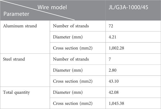
TABLE 1. Wire parameters.
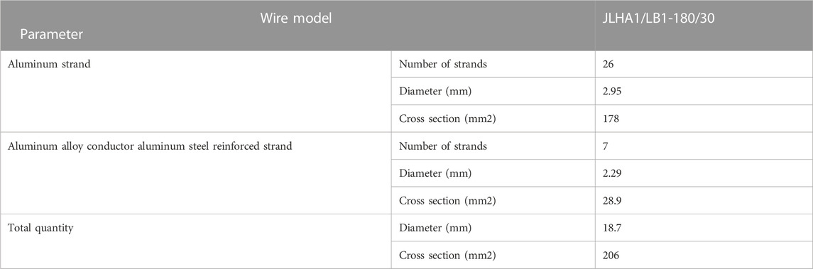
TABLE 2. Earth wire parameters.
Other parameter settings for the program are shown in Table 3.

TABLE 3. Parameter settings.
When typical ± 800 kV power lines in the high-altitude region have different heights above ground, the ground field distribution are shown in Figures 6, 7.
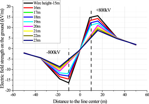
FIGURE 6. Distribution rules of ground field under ± 800 kV power lines with different heights above ground.
According to relevant national standards, for ± 800 kV UHVDC overhead transmission lines, in case of maximum sag, the minimum distance between the wire and the ground is 21 m when the lines go through the residential areas, and non-distorted total electric field on the ground shall not exceed 15 kV/m. It can be seen from Figure 7 that the total electric field on the ground increases with the wire’s decreasing height above ground. 6*JL/G3A-1000/45 steel-cored aluminum strand is adopted; when the wire height reaches 21 m, the electric field on the ground is 10.2 kV/m, which is much lower than the limit set in the national standards.
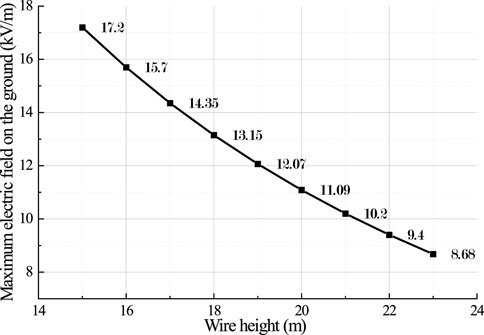
FIGURE 7. Changes in the maximum electric field on the ground under ± 800 kV power lines with different heights above ground.
The control of the ion current density on the ground under the UHVDC transmission lines relates to the personal safety of residents nearby, so it is necessary to study the ion current density features on the ground under the transmission lines.
When the distance of ± 800 kV power lines above ground is set as 21 m, changes in the ion current density on the ground with the wire’s roughness coefficient are shown in Figures 8, 9.
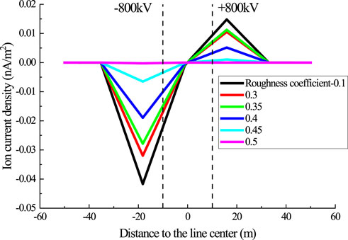
FIGURE 8. Ion current density distribution on the ground under ± 800 kV power lines with different roughness coefficients.
It can be seen from Figure 9 that the ion current density on the ground decreases with the increase in the wire’s roughness coefficient. According to the national standards, ion current density in the residential areas shall be restricted to 80 nA/m2 on sunny days. 6*JL/G3A-1000/45 steel-cored aluminum strand is adopted; when the roughness coefficient is 0.1, the maximum ion current density on the ground is
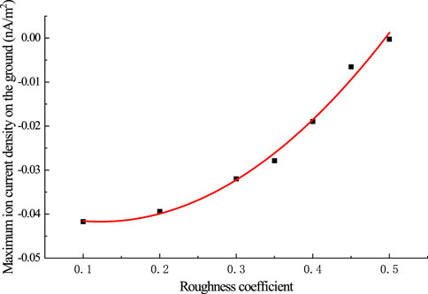
FIGURE 9. Changes in the maximum ion current density on the ground under ± 800 kV power lines with different roughness coefficients.
According to the above analyses, 6*JL/G3A-1000/45 steel-cored aluminum strand adopted for typical ± 800 kV power lines in the high-altitude region does not have serious corona, which fully meets the requirements for electric field and ion current density limits on the ground.
1) Based on the upwind difference idea proposed by Takuma, the boundary condition and initial value selection are improved with the Kaptzov hypothesis as the boundary condition, and the difference between the electric field strength on the surface of the wire and the critical coronal voltage is used as the benchmark to estimate the initial value of charge density. Thus, the calculation model of the electric field on the ground under the UHVDC lines is established, and the accuracy of the proposed model is verified;
2) By adopting the improved method, the calculation results of the total electric field and ionized field under the ± 800 kV power lines in the typical high-altitude region suggest that the total electric field on the ground decreases with the wire’s increasing height above ground and that the ion current density on the ground also decreases with the wire’s roughness coefficient;
3) When the wire height reaches 21 m, the electric field on the ground is 10.2 kV/m, which is much lower than the limit set in the national standards 15 kV/m. The 6*JL/G3A-1000/45 steel-cored aluminum strand adopted for typical ±800 kV power lines in the high-altitude region does not have serious corona, which fully meets the requirements for electric field and ion current density limits on the ground.
The original contributions presented in the study are included in the article/Supplementary Material, further inquiries can be directed to the corresponding author.
ZG: Conceptualization, methodology, investigation, software, formal analysis, writing—original draft, data curation, project administration, funding acquisition; JY: validation, methodology, writing—review and editing, data curation, investigation, software; XW: formal analysis, investigation, resources, visualization, supervision. YZ: investigation, writing—review and editing, data curation.
This work was supported by Fundamental Research Program of Shanxi Province (Grant No. 20210302123388) and Scientific research project of Shanxi Institute of Technology (Grant No. 2022010).
The authors declare that the research was conducted in the absence of any commercial or financial relationships that could be construed as a potential conflict of interest.
All claims expressed in this article are solely those of the authors and do not necessarily represent those of their affiliated organizations, or those of the publisher, the editors and the reviewers. Any product that may be evaluated in this article, or claim that may be made by its manufacturer, is not guaranteed or endorsed by the publisher.
Fu, Binlan (1993). Monopolar corona loss of Gezhouba-Nanqiao HVDC transmission line[J]. Power Syst. Technol. 17 (3), 16–21.
Hirsch, F. W., and Schafer, E. (1969). Progress Report on the HVDC test line of the 400 kV-forschungsgemeinschaft: Corona losses and radio interference. IEEE Trans. Power Apparatus Syst. 88 (7), 1061–1069. PAS-. doi:10.1109/tpas.1969.292506
Janischewskyj, W., and Cela, G. (1979). Finite element solution for electric fields of coronating DC transmission lines. IEEE Trans. Power Apparatus Syst. 98 (3), 1000–1012. PAS-. doi:10.1109/tpas.1979.319258
Liu, Zhenya (2009). Electromagnetic environment of UHVDC transmission projects [M]. Beijing, China: China Electric Power Press.
Maruvada, P. S., Dallaire, R. D., Heroux, P., and Rivest, N. (1981). Corona studies for biploar HVDC transmission at voltages between ±600 kV and ±1200 kV part 2: Special biploar line, bipolar cage and bus studies. IEEE Trans. Power Apparatus Syst. 100 (3), 1462–1471. PAS-. doi:10.1109/tpas.1981.316621
Maruvada, P. S., Trinh, N. G., Dallaire, R. D., and Rivest, N. (1981). Corona studies for biploar HVDC transmission at voltages between ±600 kV and ±1200 kV Part 1: Long-term bipolar line studies. IEEE Trans. Power Apparatus Syst. 100 (3), 1453–1461. PAS-. doi:10.1109/tpas.1981.316620
Min, L. I., Ruihai, L. I., Lei, L., Huaying, Z., Guoli, W., Xiaolin, L., et al. (2011). Electromagnetic environment measurement of ±800 kV DC transmission lines at high altitude[J]. South. Power Syst. Technol. 5 (1), 42–45.
Sarma, M. P., and Janischewskyj, W. (1969). Analysis of corona losses on DC transmission lines Part II - bipolar lines. IEEE Trans. Power Apparatus Syst. (10), 1476–1491. doi:10.1109/tpas.1969.292276
Sarma, M. P., and Janischewskyj, W. (1969). Analysis of corona losses on DC transmission lines: I - unipolar lines. IEEE Trans. Power Apparatus Syst. (5), 718–731. doi:10.1109/tpas.1969.292362
Sunaga, Y., and Sawada, Y. (1980). Method of calculating ionized field of HVDC transmission lines and analysis of space charge effects on RI. IEEE Trans. Power Apparatus Syst. 99 (2), 605–615. AS-. doi:10.1109/tpas.1980.319707
Takuma, T., Ikeda, T., and Kawamoto, T. (1982). Calculation of ion flow fields of HVDC transmission lines by the finite element method[J]. IEEE Trans. Power Apparatus Syst. 100 (12), 4802–4810. PAS-.
Wang, Donglai, Lu, Tiebing, Chen, Bo, Li, X., Xie, L., Zhao, L., et al. (2019). Ion flow field distribution near the crossing of two circuit UHVDC transmission lines. Int. J. Appl. Electromagn. Mech. 59 (2), 407–415. doi:10.3233/jae-171145
Wang, Donglai, Lu, Tiebing, Wang, Yuan, Chen, B., and Li, X. (2018). Measurement of surface charges on the dielectric film based on field mills under the HVDC corona wire. Plasma Sci. Technol. 20 (5), 054008. doi:10.1088/2058-6272/aaac26
Keywords: high altitude, UHVDC transmission line, total electric field, ionized field, minimum height above ground
Citation: Guo Z, Yu J, Wang X and Zhang Y (2023) Research on minimum height above ground considering total and ionized field when ± 800 kV power lines at the high altitude cross the residential areas. Front. Energy Res. 11:1123548. doi: 10.3389/fenrg.2023.1123548
Received: 14 December 2022; Accepted: 10 March 2023;
Published: 22 March 2023.
Edited by:
IMR Fattah, University of Technology Sydney, AustraliaReviewed by:
Mario J. Pinheiro, University of Lisbon, PortugalCopyright © 2023 Guo, Yu, Wang and Zhang. This is an open-access article distributed under the terms of the Creative Commons Attribution License (CC BY). The use, distribution or reproduction in other forums is permitted, provided the original author(s) and the copyright owner(s) are credited and that the original publication in this journal is cited, in accordance with accepted academic practice. No use, distribution or reproduction is permitted which does not comply with these terms.
*Correspondence: Zhijian Guo, d3NzbDEwMzA1MEAxNjMuY29t
Disclaimer: All claims expressed in this article are solely those of the authors and do not necessarily represent those of their affiliated organizations, or those of the publisher, the editors and the reviewers. Any product that may be evaluated in this article or claim that may be made by its manufacturer is not guaranteed or endorsed by the publisher.
Research integrity at Frontiers
Learn more about the work of our research integrity team to safeguard the quality of each article we publish.