Evaluation of the impact of inertia on system operation cost

The inertia of the power system currently lies in a relatively narrow range. However, the increasing penetration of distributed energy resources (DERs) will significantly reduce the inertia level, meanwhile increasing its volatility. This will affect the system’s ability to contain the maximum frequency excursion and recover from large frequency disturbances. In order to maintain system frequency security and stability, a common practice is to incorporate frequency security constraints into the unit commitment (UC) model, so a concern is how the volume and volatility of system inertia impact system operation costs and energy clearing prices. Furthermore, inertia forecasting is often required when performing day-ahead UC with frequency security constraints. Therefore, this paper aims to evaluate the impact of system inertia on system operation costs and energy clearing prices. The experiment is designed under scenarios with different inertia volume, inertia volatility, and inertia forecasting errors. The results show that: 1) Increasing the system inertia volume can effectively reduce the system operation costs and energy clearing prices. 2) Increasing the inertia volatility will lead to an increase in system operation costs and energy clearing prices. 3) The increment of system operation cost caused by positive or negative errors of inertia forecasting is asymmetric.

1 Introduction

Inertia is an inherent property of an object, expressed as the degree of resistance to a change in state of motion. Power system inertia is the resistance to frequency changes caused by external disturbances, which is an important guarantee for system frequency stability (Ekanayake and Jenkins, 2004). As the penetration of distributed energy resources (DERs) represented by wind power and photovoltaic power continues to increase, the system inertia level will be significantly reduced while increasing its volatility (Tielens and Van Hertem, 2016). The system inertia level will directly affect the day-ahead and real-time scheduling decisions and further affect the system operation costs. Therefore, it is necessary to evaluate the impact of system inertia on system operation costs in various scenarios.

At present, the research works related to power system inertia can be divided into four categories. The first category is equivalent inertia online evaluation. This category of work is based on the system time-domain response data measured by the phasor measurement unit (PMU) after the disturbance, combined with the system equivalent aggregation model, and uses parameter identification technology to realize the online evaluation of the system equivalent inertia. According to the type of disturbance, the existing inertia evaluation methods can be divided into three categories: evaluation methods based on frequency events (Inoue et al., 1997), evaluation methods based on small disturbance events (Wall and Terzija, 2014) and evaluation methods based on the quasi-steady-state operation (Tuttelberg et al., 2018). The second category is the system minimum inertia requirement calculation. At present, the system minimum inertia requirement is usually calculated using the rate of change of frequency (RoCoF) in the inertia response stage and the frequency nadir in the primary frequency regulation stage as key indicators to avoid triggering the frequency protection device action during the frequency response. In the literature study by (Tielens, 2017), the European power system is taken as the research object, and the system minimum inertia requirement is calculated when the RoCoF threshold is 1 Hz/s under different disturbance power conditions. In the literature study by (Golpîra et al., 2016), the RoCoF and the frequency nadir constraints are considered to calculate the system minimum inertia requirement. The third category focuses on improving the inertia support capability of the power system. In the literature study by (Chen et al., 2016), the compressed air energy storage and pumped-hydro storage are used to provide inertia support. In addition, as a synchronous grid-connected device, the synchronous condenser (SC) also stores rotational kinetic energy during rated operation. The SC has the same voltage source characteristics as synchronous generators, which can release rotational kinetic energy to provide inertia support (Yan et al., 2015). The virtual inertia control technology based on the rotor motion equation of the synchronous generator, making the grid-connected devices can simulate the electromechanical swing process of the synchronous generator to provide inertia support (Rezkalla et al., 2018). The fourth category is the optimal operation of power system based on inertia. In order to coordinate the contradiction between power system frequency security and economic benefits, the existing works regard the economic benefits of power system operation as the optimization objective, and use the frequency security constraints as boundary conditions to construct the unit commitment (UC) model. In the literature study by (Ahmadi and Ghasemi, 2014), the frequency nadir constraint is converted to an inertia constraint and incorporated into the UC model. In the literature study by (Fang et al., 2019), the system frequency response model, which can accurately reflect the relationship between inertia and frequency response, is incorporated into the UC model.

However, few studies have focused on the impact of system inertia on system operation cost and energy clearing price. For example, how the volume of system inertia and its volatility impacts the system operation costs and energy clearing prices. Furthermore, when performing day-ahead UC with frequency security constraints, the forecasting of future inertia levels is required, whereas inaccurate inertia forecasts will lead to extra or improper scheduling and increase system operation costs. Inertia forecasting errors will result in increased costs, but the increased costs caused by positive or negative errors may be asymmetric. That is, higher inertia forecasting errors do not necessarily lead to higher system operation costs. Therefore, this paper will analyze the impact of system inertia on system operation costs from three aspects: 1) The impact of the system inertia volume on system operation costs and energy clearing prices. 2) The impact of the volatility of the system inertia on system operation costs and energy clearing prices. 3) The impact of system inertia forecasting errors on system operation costs.

The rest of the paper is organized as follows: Section 2 describes the definition of system inertia and its role in the frequency response process. Section 3 describes the UC model with frequency security constraints. Section 4 analyzes the impact of system inertia on system operation cost and energy clearing price, and Section 5 makes the conclusions of the work.

2 The role of power system inertia in frequency response processes

After a disturbance occurs in the power system, the typical frequency response time axis is shown in Figure 1. The dynamic process of frequency response is mainly divided into two stages: inertia response and frequency regulations (Dreidy et al., 2017).

FIGURE 1

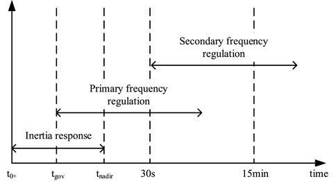
FIGURE 1. Typical timing diagram of frequency response.

2.1 Definition of system inertia

System inertia is used to describe all forms of inertia in a power system. For synchronous generators, the inertia can be described by the moment of inertia, and the inertia is reflected in the degree of resistance to changes in rotational speed, which is expressed as:

$J=\int r^{2}dm(1)$

where r is the radius of rotation. m is the mass of the rigid body. For a generator i, its moment of inertia is constant, and the kinetic energy stored in its rotor rotation is:

$E_i=\frac{1}{2}{J}_i{{\omega }_i}^2(2)$

where ω_i is the mechanical angular velocity of a single machine i. The generator kinetic energy E_i depends on the moment of inertia and the rotational speed, and is not related to the actual output power. For a generator operating at rated power, the kinetic energy depends only on its moment of inertia. The total generator inertia H_g can also be expressed as follow:

$H_g=\frac{\sum E_i}{f_0}=\frac{\sum H_i{S}_i{I}_i}{f_0}(3)$

where S_i is the rated capacity of a single machine i. H_i is the inertia constant of a single machine (seconds) with base of machine’s rated capacity. I_i is the operation status of generator i with 0/1 indicating generator being offline/online. For power electronic interface sources, its inertia forms are various and its inertia characteristics are no longer limited to the moment of inertia, but depend on the control mode of the converter and its operating state. The inertia provided by the power electronics interface sources is called virtual inertia.

In this paper, we define the system inertia as the sum of the inertia of the synchronous generators and the virtual inertia of the power electronics interface sources. The system inertia is defined as follows:

$H_{sys}=H_g+H_e(4)$

where H_e is the virtual inertia provided by power electronics interface sources.

2.2 System inertia response

When an active imbalance disturbance occurs in the system, each synchronous generator instantaneously shares the disturbance power according to its synchronous power coefficient. After that, the electromagnetic power of the i-th generator changes suddenly, while the mechanical power remains unchanged. The rotor motion state will change according to the rotor motion equation under the action of unbalanced torque:

$2H_i\frac{d∆f_i\left(0^{+}\right)}{dt}=-∆P_i^L\left(0^{+}\right)(5)$

where H_i represents the inertia of generator i. $∆f_i\left(0^{+}\right)$ represents the frequency deviation of generator i at time 0⁺. t represents time. $∆P_i^L\left(0^{+}\right)$ represents the power change of generator i at time 0⁺. The difference among the inertia of the generators leads to different rotor speeds of the generators, but the effect of the synchronous torque will make the rotor speeds tend to be consistent. Therefore, each generator will re-share the disturbance power according to the generator inertia:

$∆P_i^L\left(t\right)=∆P_L\cdot \frac{H_i}{{\sum }_{i=1}^N{H}_i}(6)$

where N represents the number of generators. $∆P_L$ represents the disturbance power. The inertia response begins when the electromagnetic power changes suddenly due to the disturbance power $∆P_L$, and ends when the frequency nadir, i.e., the balance between the electromagnetic power and the mechanical power, is reached. As shown in Figure 1, the overall process can be divided into two stages:

(1) t₀₊ ∼ t_gov: The moment of distribution of the disturbance power to the moment when the governor starts to act. The inertia of synchronous generators responds to support system power balance.

(2) t_gov ∼ t_nadir: The moment when the governor starts to act to the moment when the frequency nadir is reached. The inertia response and the primary frequency regulation jointly support the system power balance.

Note that this paper only describes synchronous generator inertia supporting power balance, but virtual inertia can also play a similar role. The virtual inertia can be divided into current-sourced virtual inertia and voltage-sourced virtual inertia. The current-sourced virtual inertia controls the active power by measuring the system frequency and feeding it back to the converter. The voltage-sourced virtual inertia mainly refers to virtual synchronous generator technology (VSG). The VSG, also known as the synchronous converter, refers to the introduction of synchronous generator rotor motion and electromagnetic transient equations in the control link of the converter so that it can simulate the voltage-sourced characteristics of the synchronous generator.

3 Unit commitment model with frequency security constraints

3.1 Frequency security constraints

The frequency response of the power system in the actual operation process actually reflects the physical process of the frequency transition from the initial steady state to the new frequency steady state after the system active power balance equation is not satisfied. The role of the frequency security constraints is to guarantee the security, and stability of the system frequency during the above process (Muzhikyan et al., 2018).

As shown in Figure 2, the inertia response occurs first to ensure the balance of electromagnetic power and mechanical power. Then, the primary frequency regulation starts to restore the frequency from the frequency nadir to the quasi-steady state. In the process of frequency response, three key metrics are used to evaluate the stability of system frequency, i.e., the rate of change of frequency (RoCoF), the frequency nadir (f_nadir), and the steady-state frequency deviation (f_ss). These three key metrics need to meet the frequency limits set by the National Grid.

(1) Rate of change of frequency (Chu et al., 2020): ROCOF indicates the slope (Hz/s) of frequency drop, and its value is related to the system inertia and power deficit. The mathematical formulation can be expressed as follow:

$RoCoF=-\frac{∆P_L}{2H_{sys}}(7)$

(2) Frequency nadir (Badesa et al., 2019): f_nadir indicates the lowest point of the frequency before the system frequency recovers. The mathematical formulation can be expressed as follow:

$f_{nadir}=\frac{∆P_L^2{T}_d}{4H_{sys}R}(8)$

where T_d is the fully delivered time of primary frequency response. R is the frequency regulating reserve.

(3) Steady-state frequency deviation (Teng et al., 2016): f_ss indicates the deviation between the frequency value after frequency recovery and the rated frequency value, which is used to reflect the primary frequency regulation effect. The mathematical formulation can be expressed as follow:

$f_{ss}=\frac{∆P_L-R}{D{P}_D}(9)$

where D is the load-dependent damping in the system. P_D is the active power demand.

FIGURE 2

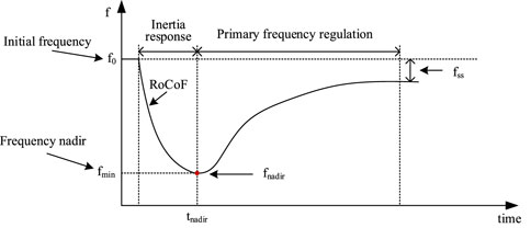
FIGURE 2. Frequency response process after power shortage.

3.2 Unit commitment model

The UC model combined with frequency security constraints is as follows:

$\underset{P_i^t,I_i^t}{\min }{\displaystyle \sum }_{t=1}^T{\displaystyle \sum }_{i=1}^N\left[C_i{P}_i^t{I}_i^t+S{U}_i{I}_i^t\left(1-I_i^{t-1}\right)\right](10)$

subject to

${\sum }_{i=1}^N{I}_i^t{P}_i^t=D^t(11)$

${\sum }_{i=1}^N{I}_i^t{P}_{i,\max }^t-D^t\ge R^t(12)$

$P_{i,\min }^t{I}_i^t\le P_i^t\le P_{i,\max }^t{I}_i^t(13)$

$\left(X_{i,on}^{t-1}-T_{i,on}\right)\cdot \left(I_i^{t-1}-I_i^t\right)\ge 0(14)$

$\left(X_{i,off}^{t-1}-T_{i,off}\right)\cdot \left(I_i^t-I_i^{t-1}\right)\ge 0(15)$

$0\le P_i^t-P_i^{t-1}\le U{R}_i(16)$

$0\le P_i^{t-1}-P_i^t\le D{R}_i(17)$

$-\frac{∆P_L}{2H_{sys}}\le ∆{\dot{f}}_{\lim }(18)$

$\frac{∆P_L^2{T}_d}{4H_{sys}R}\le ∆f_{\lim }(19)$

$\frac{∆P_L-R}{D{P}_D}\le ∆f_{\lim }^{ss}(20)$

where C_i is the marginal cost of generator i. $P_i^t$ and $I_i^t$ are the output power and on-off state of generator i at time t, respectively. SU_i is the startup cost of generator i. D^t and R^t are load demand and reserve demand at time t, respectively. $P_{i,\min }^t$ and $P_{i,\max }^t$ are the minimum and maximum active output of generator i at time t, respectively. UR_i and DR_i are the ramping-up rate and ramping-down rate of generator i, respectively. $T_{i,on}$ and $T_{i,off}$ are the minimum on and off requirements of generator i, respectively. $X_{i,on}^{t-1}$ and $X_{i,off}^{t-1}$ are the continuous running time and downtime of the generator i, respectively. $∆{\dot{f}}_{\lim }$, $∆f_{\lim }$ and $∆f_{\lim }^{ss}$ are the maximum permissible RoCoF, maximum permissible frequency deviation and maximum permissible steady-state frequency deviation, respectively.

The objective (10) is to minimize the total operation cost including startup and generation costs. Constraint (11) ensures active power balance. Constraint (12) ensures sufficient reserve capacity. The generator constraints include generation limits (13), minimum on and off requirements (14)-(15), and ramping limits (16)-(17). Constraint (18) ensures that the RoCoF is within the allowed deviation range. Constraint (19) ensures that the frequency deviation is within the allowed deviation range. Constraint (21) ensures that the steady-state frequency deviation is within the allowed deviation range.

3.3 Calculation of energy clearing price and system operation cost

In this paper, we defined the dual multipliers of constraint (11) as the energy clearing price, which can be obtained by solving the dual problem of the above model.

The system operation cost is obtained by solving day-ahead UC and real-time economic dispatch (ED). Specifically, since H_e remains unknown in the day-ahead stage, UC is first conducted to clear the day-ahead market, providing the actual UC cost, i.e., start-up cost. After H_e is realized in the real-time stage, ED is executed to clear the real-time market, providing the actual ED cost, i.e., generation cost for all units. Therefore, the system operation cost is equal to the sum of the actual UC cost and the actual ED cost. The simplified ED model is as follows:

$\underset{P_i^t}{\min }{\displaystyle \sum }_{t=1}^T{\displaystyle \sum }_{i=1}^N\left[C_i{P}_i^t{I}_i^{t\ast }\right](21)$

subject to

${\sum }_{i=1}^N{I}_i^{t\ast }{P}_i^t=D^t(22)$

${\sum }_{i=1}^N{I}_i^{t\ast }{P}_{i,\max }^t-D^t\ge R^t(23)$

$P_{i,\min }^t{I}_i^{t\ast }\le P_i^t\le P_{i,\max }^t{I}_i^{t\ast }(24)$

$\mathrm{c}\mathrm{o}\mathrm{n}\mathrm{s}\mathrm{t}\mathrm{r}\mathrm{a}\mathrm{i}\mathrm{n}\mathrm{s}\left(16\right)-\left(20\right)(25)$

where $I_i^{t*}$ is the solution of the UC model. Therefore, the system operation cost can be calculated as follows:

$\mathrm{c}\mathrm{o}\mathrm{s}\mathrm{t}={\displaystyle \sum }_{t=1}^T{\displaystyle \sum }_{i=1}^N\left[C_i{P}_i^{t*}{I}_i^{t\ast }+S{U}_i{I}_i^{t\ast }\left(1-I_i^{t-1}\right)\right](26)$

where $P_i^{t*}$ is the solution of the real time ED model.

4 Analysis of the impact of system inertia on system operation costs and energy prices

In this section, we will analyse the impact of system inertia on system operation costs and energy clearing prices. Mainly include: 1) The impact of the system inertia volume on system operation costs and energy clearing prices. 2) The impact of the volatility of the system inertia on system operation costs and energy clearing prices. 3) The impact of system inertia forecasting errors on system operation costs. Note that since the inertia of the synchronous generator is determined by the on-off state of the generator, what we call changing the system inertia refers to changing the virtual inertia.

4.1 Experimental setting

Several case studies of the modified GB 2030 power system are carried out to analyze the impact of system inertia on system operation costs (Teng et al., 2016). The characteristics of generation plants are included in Table 1. The system includes nuclear power generators, open-cycle gas turbines (OCGTs), and combined-cycle gas turbines (CCGTs). OCGTs can be regarded as slow synchronous generators with low marginal cost and CCGTs can be regarded as faster synchronous generators with higher marginal cost. The system parameters are set as follows: load demand P_D∈ [20, 60] × 10³ MW, damping D = 0.5% P_D/1 Hz, frequency response delivery time T_d = 10 s and maximum power loss ΔP_L = 2100 MW. The frequency limits set by National Grid are: $\Delta f_{\lim }$ = 0.8 Hz, $\Delta f_{\lim }^{ss}$ = 0.5 Hz, and $\Delta {\dot{f}}_{\lim }$ = 0.5 Hz/s. The simulation adopts day-ahead scheduling, with a total duration of 24 h and a time interval of 1 h.

TABLE 1

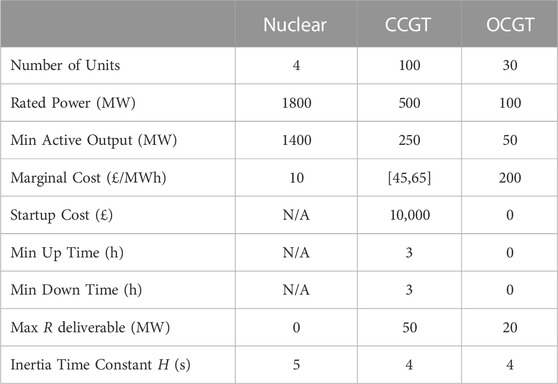
TABLE 1. Characteristics of thermal plants in GB’s 2030 system.

4.2 The impact of the system inertia volume on system operation costs and energy clearing prices

We first set the system inertia at each moment to be the same, and then gradually increase the system inertia to observe the change in system operation cost. As shown in Figure 3, with the gradual increase of inertia, the overall system operation cost presents a downward trend. This is because the frequency security constraints will be easily satisfied when the system inertia is sufficient, resulting in fewer CCGTs being turned on in the day-ahead decisions to provide inertia and frequency regulating reserve. It is also worth noting that there is not a linear relationship between system inertia and system operation costs. It can be seen from Figure 4 that with the increase of the system inertia volume, the energy clearing price decreases, and the decrease is particularly obvious in the shaded area. This is because without additional inertia support, satisfying the system frequency security constraints would require OCGTs with higher marginal costs to be online to provide inertia and frequency regulating reserves support. And when the system inertia volume increases, OCGTs do not need to be scheduled.

FIGURE 3

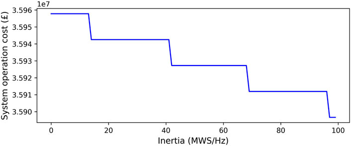
FIGURE 3. Impact of inertia volume on system operation costs.

FIGURE 4

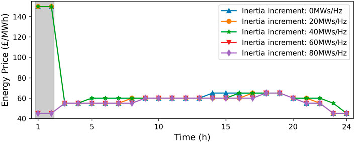
FIGURE 4. Impact of inertia increment on energy prices.

4.3 The impact of the volatility of the system inertia on system operation costs and energy clearing prices

We first set the system inertia at each moment to be a normal distribution with a mean of 50 (MWs/Hz), and then gradually increase the standard deviation of the system inertia to observe the change of system operation costs. As shown in Figure 5, as the volatility of inertia gradually increases, the system operation cost shows an upward trend. This is because the greater the volatility of the system inertia, the more CCGTs are required to be online for day-ahead scheduling decisions, thus resulting in expensive start-up costs. It can be seen from Figure 6 that the energy clearing price increases in some time periods as the standard deviation of inertia increases. This is because due to the constraints of ramping and minimum on and off requirements, the units cannot instantly provide inertia support when the system inertia volume is insufficient, and therefore more units are required online to cope with the volatility of the system inertia, resulting in increased energy clearing prices.

FIGURE 5

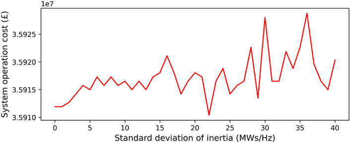
FIGURE 5. Impact of the standard deviation of inertia on system operation costs.

FIGURE 6

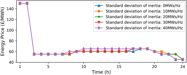
FIGURE 6. Impact of the standard deviation of inertia on energy prices.

4.4 The impact of system inertia forecasting errors on system operation costs

When making day-ahead decision-making, the virtual inertia in the system inertia needs to be forecasted. This is because virtual inertia depends on multiple factors, such as weather-dependent non-synchronous sources, load, market forces, etc. The system operation cost caused by the inertia forecasting error may be asymmetric, so it is necessary to analyze the impact of the inertia forecasting errors on the system operation costs.

We set the true value of the system inertia to 250 (MWs/Hz), and the system operation cost caused by the forecasted error is shown in Figure 7. Figure 7A shows the impact of system inertia forecasting errors on system operation costs for the high average load scenario. The under-forecasting of inertia in this scenario does not result in an increase in system operation costs, as the units being dispatched satisfy the power demand while also satisfying the day-head and real time frequency security constraints. However, over-forecasting the inertia will lead to higher system operation costs, because the real-time frequency security constraints may not be satisfied, so high-cost OCGTs with fast responding capability have to be dispatched online for inertia provision, resulting in a significant increase in system operation costs. Figure 7B shows the impact of system inertia forecasting errors on system operation costs for the low average load scenario, the under-forecasting of inertia results in more CCGTs being prepared during day-ahead scheduling, leading to less efficient part-loading operation. Figures 7C, D show the impact of the system inertia forecasting errors on the system operation costs when the marginal cost of OCGT is 75£/MWh and 300£/MWh, respectively. It can be seen that an increase in the marginal price of OCGT causes an increase in the cost of ED, thereby further increasing the system operation costs.

FIGURE 7

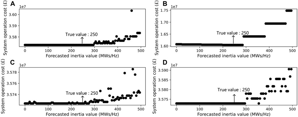
FIGURE 7. Impact of inertia forecasting errors on system operation costs.

5 Conclusion

This paper evaluates the impact of system inertia on system operation costs and energy clearing prices, and draws the following conclusion:

1) Increasing the system inertia volume can effectively reduce the system operation cost, while decreasing the energy clearing prices. The relationship between system inertia volume and system operation cost is not linear.

2) Increasing the volatility of system inertia will lead to an increase in system operation cost and energy clearing price. Because more CCGTs need to be prepared in the day-ahead scheduling stage for the volatility of inertia.

3) The system operation cost caused by forecasting error is asymmetric, and the system operation cost caused by over-forecasting is much higher than that caused by under-forecasting. Because over-forecasting will lead to insufficient real-time inertia, the high-cost OCGTs with fast response capability need to be dispatched online for inertia provision, resulting in a significant increase in system operation costs.

Data availability statement

The original contributions presented in the study are included in the article/supplementary material, further inquiries can be directed to the corresponding author.

Author contributions

The author’s personal contributions are as follows: manuscript writing and data collection: LZ, HW, and YW; content and format correction: HZ, WL, and RL all authors have read and agreed to the published version of the manuscript.

Funding

This paper is funded by project JY02202269 which is provided from Zhejiang Electric Power Company Economic and Technological Academe.

Conflict of interest

Authors LZ, HW, and YW were employed by State Grid Zhejiang Electric Power Co., Ltd.

The remaining authors declare that the research was conducted in the absence of any commercial or financial relationships that could be construed as a potential conflict of interest.

The authors declare that this study received funding from Zhejiang Electric Power Company. The funder had the following involvement in the study: they collaboratively conceived the study and collected the experimental data. LZ advised on the analysis and reviewed the manuscript.

Publisher’s note

All claims expressed in this article are solely those of the authors and do not necessarily represent those of their affiliated organizations, or those of the publisher, the editors and the reviewers. Any product that may be evaluated in this article, or claim that may be made by its manufacturer, is not guaranteed or endorsed by the publisher.

References

Ahmadi, H., and Ghasemi, H. (2014). Security-constrained unit commitment with linearized system frequency limit constraints. IEEE Trans. Power Syst. 29 (4), 1536–1545. doi:10.1109/tpwrs.2014.2297997

CrossRef Full Text | Google Scholar

Badesa, L., Teng, F., and Strbac, G. (2019). Simultaneous scheduling of multiple frequency services in stochastic unit commitment. IEEE Trans. Power Syst. 34 (5), 3858–3868. doi:10.1109/tpwrs.2019.2905037

CrossRef Full Text | Google Scholar

Chen, L., Zheng, T., Mei, S., Xue, X., Liu, B., and Qiang, L. (2016). Review and prospect of compressed air energy storage system. J. Mod. Power Syst. Clean Energy 4 (4), 529–541. doi:10.1007/s40565-016-0240-5

CrossRef Full Text | Google Scholar

Chu, Z., Markovic, U., Hug, G., and Teng, F. (2020). Towards optimal system scheduling with synthetic inertia provision from wind turbines. IEEE Trans. Power Syst. 35 (5), 4056–4066. doi:10.1109/tpwrs.2020.2985843

CrossRef Full Text | Google Scholar

Dreidy, M., Mokhlis, H., and Mekhilef, S. (2017). Inertia response and frequency control techniques for renewable energy sources: A review. Renew. Sustain. Energy Rev. 69, 144–155. doi:10.1016/j.rser.2016.11.170

CrossRef Full Text | Google Scholar

Ekanayake, J., and Jenkins, N. (2004). Comparison of the response of doubly fed and fixed-speed induction generator wind turbines to changes in network frequency. IEEE Trans. Energy Convers. 19 (4), 800–802. doi:10.1109/tec.2004.827712

CrossRef Full Text | Google Scholar

Fang, J., Zhang, R., Li, H., and Tang, Y. (2019). Frequency derivative-based inertia enhancement by grid-connected power converters with a frequency-locked-loop. IEEE Trans. Smart Grid 10 (5), 4918–4927. doi:10.1109/tsg.2018.2871085

CrossRef Full Text | Google Scholar

Golpîra, H., Seifi, H., Messina, A. R., and Haghifam, M. (2016). Maximum penetration level of micro-grids in large-scale power systems: Frequency stability viewpoint. IEEE Trans. Power Syst. 31 (6), 5163–5171. doi:10.1109/tpwrs.2016.2538083

CrossRef Full Text | Google Scholar

Inoue, T., Taniguchi, H., Ikeguchi, Y., and Yoshida, K. (1997). Estimation of power system inertia constant and capacity of spinning-reserve support generators using measured frequency transients. IEEE Trans. Power Syst. 12 (1), 136–143. doi:10.1109/59.574933

CrossRef Full Text | Google Scholar

Muzhikyan, A., Mezher, T., and Farid, A. M. (2018). Power system enterprise control with inertial response procurement. IEEE Trans. Power Syst. 33 (4), 3735–3744. doi:10.1109/tpwrs.2017.2782085

CrossRef Full Text | Google Scholar

Rezkalla, M., Pertl, M., and Marinelli, M. (2018). Electric power system inertia: Requirements, challenges and solutions. Electr. Eng. 100 (4), 2677–2693. doi:10.1007/s00202-018-0739-z

CrossRef Full Text | Google Scholar

Teng, F., Trovato, V., and Strbac, G. (2016). Stochastic scheduling with inertia dependent fast frequency response requirements. IEEE Trans. Power Syst. 31 (2), 1557–1566. doi:10.1109/tpwrs.2015.2434837

CrossRef Full Text | Google Scholar

Tielens, P. (2017). Operation and control of power systems with low synchronous inertia. Leuven: University of Leuven.

Google Scholar

Tielens, P., and Van Hertem, D. (2016). The relevance of inertia in power systems. Renew. Sustain. Energy Rev. 55, 999–1009. doi:10.1016/j.rser.2015.11.016

CrossRef Full Text | Google Scholar

Tuttelberg, K., Kilter, J., Wilson, D., and Uhlen, K. (2018). Estimation of power system inertia from ambient wide area measurements. IEEE Trans. Power Syst. 33 (6), 7249–7257. doi:10.1109/tpwrs.2018.2843381

CrossRef Full Text | Google Scholar

Wall, P., and Terzija, V. (2014). Simultaneous estimation of the time of disturbance and inertia in power systems. IEEE Trans. Power Deliv. 29 (4), 2018–2031. doi:10.1109/tpwrd.2014.2306062

CrossRef Full Text | Google Scholar

Yan, R., Saha, T. K., and Modi, N. (2015). “Frequency response and its enhancement using synchronous condensers in presence of high wind penetration,” in Proceeding of the 2015 IEEE Power & Energy Society General Meeting, Denver, CO, USA, July 2015 (IEEE), 1–5.

Google Scholar