 Hongtao Tan
 Hui Li*
 Zhiting Zhou
- State Key Laboratory of Power Transmission Equipment and System Security and New Technology, Chongqing University, Chongqing, China
Voltage stability region assessment is the key to ensuring the reliable operation of offshore wind farms However, the traditional analysis method, which treats the WFs as a PQ node and directly connected to the infinite power grid, fails to take the cable capacitance and the dynamics of the converter into account, resulting an inaccurate evaluation of voltage stability. The contribution of this paper is to propose a more accurate method for assessing the voltage stability of OWFs. Firstly, based on the equivalent circuit method, the point of common coupling (PCC) and internal voltage characterization models of OWF considering the cable capacitance parameters are derived. Then, the coupling interface between the dynamic of the converter and the voltage characteristics of the system is designed, and the transfer function of the power injection from the DC side of the converter to the voltage of the collector system is established, which fully reflects the OWF Pin→Udc→Id→Upcc→Pout transitive relationship. Finally, a voltage stability criterion based on dPw, out/dId&dUdc/dt direction discrimination is proposed, and the influence of cable parameters, output power, and grid impedance on the voltage stability margin is analyzed. The accuracy of the proposed method is verified based on the RT-LAB platform.
1 Introduction
As an important renewable energy, offshore wind power has the characteristics of high available hours and no land occupation. According to the data of GWEC, the newly installed capacity of global offshore wind power reached 21.1 GW in 2021, double the year-on-year growth, and the newly installed capacity of global offshore wind power will reach 33.95 GW in 2027 (Musial et al., 2022), which shows that the development prospect of offshore wind farms is very broad.
OWFs are generally developed in a centralized manner and collected to offshore booster stations, and then connected to onshore power grids through submarine cables. For OWFs (within 50 km offshore), AC submarine cable transmission and grid connection is currently the most economical transmission method (Hu et al., 2013; Elliott et al., 2016). For conventional onshore WFs, since the inductance of the onshore transmission line is much larger than the resistance parameter, the parameters of the onshore transmission cable are generally directly reduced to the grid impedance (Zhu et al., 2020; Guan et al., 2021). Therefore, the voltage stability problems of onshore WFs are mostly caused by the weak grid formed by long-distance overhead line transmission. However, unlike onshore WFs, offshore wind farms are close to the load center, but the capacitance parameter of submarine AC cable is more than 20 times that of onshore transmission lines, which makes the voltage problem also prominent (Gustavsen and Mo, 2017; Wang et al., 2019). For example, in 2019, several power frequency overvoltages occurred in Shantou OWF in Guangdong Province, which caused the OWF to be disconnected from the grid and shut down. In addition, due to the typical radial structure of OWFs and the reverse power flow of the system, the reverse voltage drop increases the risk of over-voltage in the collector system inside the WF (Zhao et al., 2016; Guo et al., 2018), so the visible voltage stability has become a key factor to restrict the safe and stable operation of OWF. Therefore, analyzing the voltage distribution characteristics and obtaining the voltage stability region is of great significance for the stable operation of OWFs and the formulation of reactive power-voltage control strategies.
PV curves (Qi et al., 2019; Chen and Han, 2020; Xu et al., 2020), critical short-circuit ratios (Xin et al., 2016; Wu et al., 2018), and bifurcation theory (Du et al., 2015) are the most common ways to evaluate the voltage stability of WFs. For example, in Xu et al. (2020), Qi et al. (2019), the PV curve of the WF grid-connected system is obtained by setting the node load to increase in the specified direction using the continuous power flow method. Chen and Han (2020) equivalent the WF as a PQ node, and the PV curve of the system is obtained based on the equivalent circuit method, and points out that as the output power increases, the system voltage gradually tends to be unstable until the voltage collapses. Similarly, the wind farm is equivalent to a PQ node, Wu et al. (2018), Xin et al. (2016) deduce the node voltage equation based on the equivalent circuit method, and propose a calculation method for the critical short-circuit ratio of the grid-connected system of the WF to evaluate the voltage support strength. Du et al. (2015) use bifurcation theory and eigenstructure method to establish a static voltage stability evaluation model for large-scale renewable energy stations, and it is pointed out that the output and cable impedance are closely related to the static voltage stability margin of the system. However, in the above studies, the wind farm nodes are equivalent to PQ nodes from the outside, and the power characteristics of the converters are not considered. The converter is the port of power injection, therefore, the power characteristics of WF converters are necessary to consider when analyzing the voltage stability.
Li et al. (2018), Kang et al. (2021), Huang and Wang (2018) take the control of the converter into account and analyze the power transmission characteristics of the converter grid-connected system. Li et al. (2018), Kang et al. (2021) take the WT converter connected to the infinite power grid system as the object, and point out that when the power grid strength is lower than a certain index, the output d-axis current (Id) and output power (Pwout) of the converter are no longer monotonically increasing, and there is a static power limit. Huang and Wang (2018) pays attention to the influence of the interaction between the control parameters of the converter and the impedance of the power grid on the transmission power characteristics, but is essentially small-signal stability, which differs greatly from the voltage stability concerned, and does not take the power dynamics on the DC-AC side of the converter into account. In addition, the above studies simplify the parameters of transmission cables as inductances and directly overlap with the inductance of an infinite power grid, while the capacitance parameter of the submarine cable is obvious and cannot be ignored. Therefore, the voltage modeling method in the above research cannot be directly applied to the analysis of the voltage characteristics of the OWF.
For the traditional static stability assessment method of wind farms, cable capacitance parameters and converter dynamics are ignored, resulting an inaccurate evaluation of voltage stability. The highlight of this paper is to propose a more accurate method for assessing the voltage stability of OWFs. The main contributions are as follows.
1) The PCC and the internal voltage model of the OWF considering the parameters of the submarine cable are established, and the influence trend of the cable parameters on the system voltage characteristics is obtained.
2) The coupling interface between the voltage of the collector system and the dynamics of the converter is designed, and the power-voltage transfer characteristics of the WT are comprehensively revealed.
3) A voltage stability criterion based on dPw, out/dId & dUdc/dt direction discrimination is proposed, and the quantitative evaluation of stability margin is realized.
The following part of this paper is organized as follows. In Section 2, the model and output characteristics for WT are introduced. The OWF Voltage model considering submarine cable parameters is introduced in Section 3. Section 4 introduces the voltage stability criterion and power limit calculation of OWF. RT-LAB experimental verification is introduced in Section 5. Section 6 concludes this paper.
2 Modeling of output characteristics of WT converter
Taking the H3 OWF (5 MW*80 units) put into operation by CSSC as the analysis object, the OWF adopts a typical radial structure, and the topology is shown in Figure A1 in Appendix A. The WT is connected to the offshore booster station by a 35 kV cable, and is boosted to 220 kV by the main transformer of the OWF and then transmitted to the onshore switch station through a 220 kV submarine cable.
The wind farm uses a 5 MW permanent magnet generator, which is connected to the grid through a full-power converter. Due to the decoupling effect of the DC link, the WT can be simplified to a structure in which the current source is connected to the grid through the grid-side converter. The grid side converter adopts a typical phase-locked follow grid control structure based on dq rotation coordinates. The control block diagram is shown in Figure 1. In the grid-side converter control, the dq rotating coordinate system is oriented by tracking the voltage vector of the PCC through the phase-locked loop. Dq component represents the active and reactive components injected into the AC power grid by the grid side converter, that is, the grid connected converter can be equivalent to the current source structure with output Id + jIq (Cespedes and Sun, 2014; Hou et al., 2019).
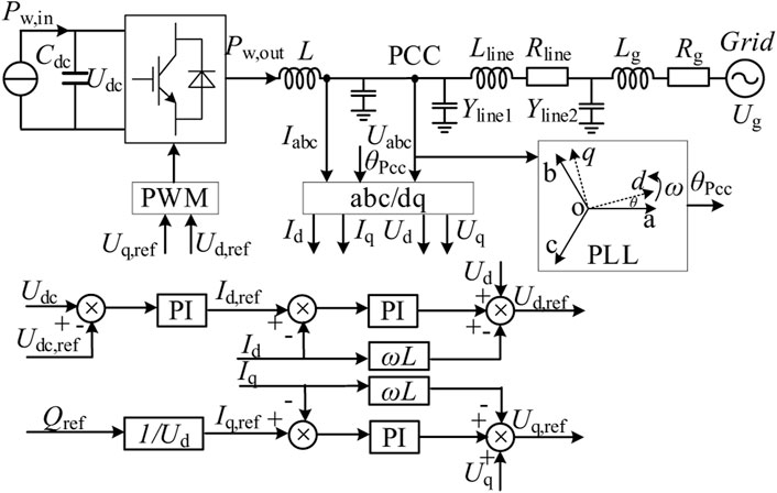
FIGURE 1. Control block diagram of WT grid-side converter.
The abbreviations of parameters in Figure 1 are explained in Table 1. In the steady-state, when the wind speed changes, the injected power (Pw, in) at the DC side of the converter changes (Kang et al., 2020). At this time, there is unbalanced power (Pw, in-Pw, out) in the DC link of the converter, and the unbalanced power will change the DC bus voltage (Udc), the change rule (ignoring the converter loss) is shown in (1):
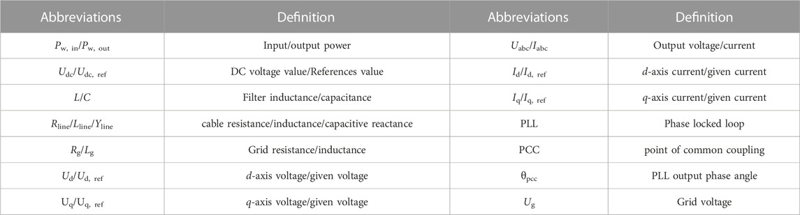
TABLE 1. Definition of parameters abbreviations.
Under steady-state operating conditions, assuming that the current loop can ideally follow its reference value, that is, Id = Id, ref, Iq = Iq, ref, the output current of the converter is:
where kp and ki are the PI parameters of the DC voltage control loop.
The output power of the converter is expressed as:
To sum up, the power input and output characteristics of the WT converter are composed of Eqs. 1—3.
3 OWF voltage modeling considering submarine cable parameters
3.1 PCC voltage modeling for OWFs
The external characteristics of the WT can be simplified as an equivalent current source with an output of Id + jIq. Figure 1 can be converted into the grid-connected equivalent circuit diagram of the WT shown in Figure 2. Among them, the OWF is equivalent to the current source with the output current is IPCC and the terminal voltage is UPCC, and then connected to the power grid with impedance is Zg and voltage is Ug through the submarine cable.
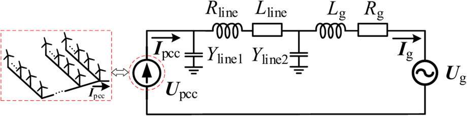
FIGURE 2. Equivalent current of AC side of OWF.
According to Figure 2, using the two-port network voltage and current coupling model, the wind farm PCC voltage relationship can be expressed as:
In (4), IPCC and Ug are known quantities and UPCC is an unknown quantity. The expression of U UPCC can be obtained by converting (4).
Where, the matrix elements A, B, C, and D are obtained from the calculation of cable parameters:
In (5), the preceding coefficients of Ug and IPCC on the right side of the equation can be obtained by calculating cable parameters and grid impedance parameters. Let a, b, c, and d be the real and imaginary parts of the preceding coefficients of Ug and IPCC respectively, that is:
Combined with (7) and the mathematical model of the converter under the dq-PLL coordinate system, the (5) can be further rewritten as:
During steady-state operation,
Expand (9) to:
According to the equality of the real and imaginary parts on both sides of (10) (see Appendix A for the specific derivation process), we get:
Combining (10) and (11) can obtain the voltage model of the PCC:
According to (12), it can directly reflect the influence of multiple parameters of grid impedance, cable parameters, and injected dq-axis current (i.e. active and reactive power) on the PCC voltage of the OWF. The relationship curve of Id-UPCC of the OWF is drawn as shown in Figure 3.
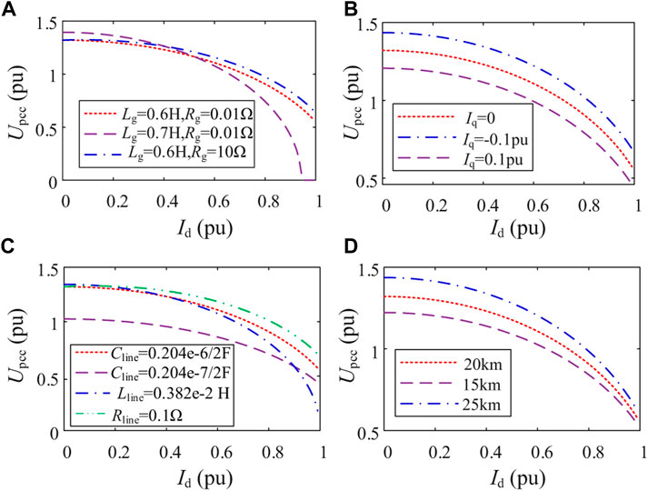
FIGURE 3. Id-UPCC curve under different parameters. (A) Grid impedance, (B) reactive current, (C) submarine cable parameters, (D) cable length.
In Figure 3, if there is no marked parameter value, use the value given in Table 2 (to more clearly describe the change relationship between PCC voltage and parameters, the value of grid impedance is 0.6H, which may not represent a real situation.). As shown in Figure 3, UPCC shows a downward trend with the increase of Id. Under different parameter settings, the amplitude and downward trend of UPCC are different. The change trend statistics are shown in Table 3. It is worth noting that the submarine cable capacitor will increase the amplitude of UPCC and slow down the falling speed of UPCC, which may cause UPCC to exceed the upper limit at low wind speeds, but increases the voltage stability of high wind speeds.
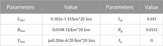
TABLE 2. Id-UPCC curve calculation parameters settings in Figure 3.

TABLE 3. Variation trend of parameters and UPCC.
3.2 Modeling of voltage distribution characteristics in OWF
The distribution of WTs and line connections in OWFs are mostly radial. Therefore, the following takes the voltage distribution of WTs on a feeder as an example to analyze the internal voltage distribution characteristics of OWFs. Figure 4 shows the equivalent circuit of a feeder in the OWF, where point O is the PCC of OWF, nodes one to five are the WT power injection nodes, and the injection current of the i-th node is the sum of the output current of the i-th WT (Iwt, i) and the injection current of the upstream node (Ii-1).
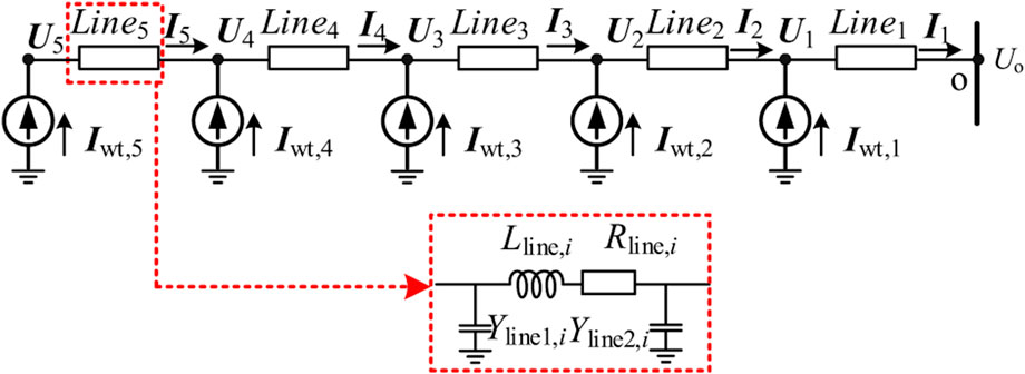
FIGURE 4. Equivalent circuit of a feeder in the OWF.
According to Figure 4, the voltage Ui of the i-th WT is.
Where the calculation of matrix elements is the same as (4). From (13), it can be known that the voltage distribution at the terminal of the WT first depends on the voltage UO at the PCC of the OWF, and is also related to the active and reactive power output of the WT and the parameters of the collector network. The influence trend of the parameters of the cable on the internal voltage distribution is consistent with (12). Therefore, the voltage distribution of the WT gradually increases from the PCC to the end of the collector feeder, that is, PCC is the voltage weakness of the OWF.
4 Voltage stability criterion and power limit calculation of OWF
4.1 Voltage stability criterion
Combining (3) and (12), the output power characteristics of the OWF can be obtained, as shown in (14):
From this, the Power-Voltage characteristic transfer function block diagram of the OWF grid-connected system is obtained, as shown in Figure 5. Where x is the input of submarine cable parameters and grid impedance parameters in (12). It can be seen that the Power-Voltage characteristics of the OWF are composed of the DC dynamic characteristics of the converter Eqs. 1-3 and the voltage characteristics of the collector system (Eq.12). The DC dynamic characteristics reflect the DC bus voltage dynamics caused by the imbalance of the input and output power of the converter, and the system voltage characteristics reflect the voltage change dynamics caused by power injection, and they are coupled with each other, that is, the increase of active power will lead to the decrease of PCC voltage, and the decrease of PCC voltage will affect the active power transmission capability of wind power converter.
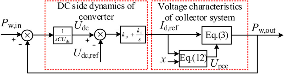
FIGURE 5. Power-Voltage characteristic transfer function block diagram of OWF.
From the functional relationship of (14), the change curve of Pw, out-Id of the wind farm can be drawn, as shown in Figure 6. It can be seen from Figure 6 that the changing trend of the Pw, out-Id curve is divided into two regions.
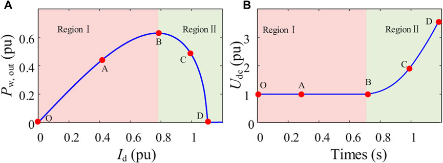
FIGURE 6. Power characteristic curve of OWF, (A) Pw, out-Id characteristic curve, (B) Udc-t characteristic curve.
In region I, Pw, out increases with the increase of Id, that is, when the DC side injection power Pw, in increases, the inner loop current Id increases under the control of DC voltage link. Although the increase of Id will lead to the decrease of terminal voltage, the output power still increases at this time, and the change trend is positive (dPw, out/dId>0). The input and output power of the DC link of the converter is balanced (Pw, in = Pw, out), and the OWF can operate stably in this area (O-A-B).
In region II, Pw, out decreases with the increase of Id, that is, when the DC side injection power Pw, in increases, the inner loop current Id increases, but at this time the output power Pw, out decreases, that is, the change trend is negative (dPw, out/dId<0), there is unbalanced power in the DC link (Pw,in > Pw, out), which will cause the DC capacitor of the converter to continuously charge and the Udc continuously increase (dUdc/dt>0). There is no stable equilibrium point for the OWF in this area, i.e. is unstable (B-C-D).
Therefore, it is possible to determine whether the voltage of the OWF is stable by obtaining the directions of dPw, out/dId and dUdc/dt.
1) dPw, out/dId>0&dUdc/dt = 0, Voltage stability (region I).
2) dPw, out/dId<0&dUdc/dt>0, Voltage instability (region II).
3) dPw, out/dId = 0, critically stable (point B).
In this paper, the distance from dPw, out/dId to 0 is defined as the quantitative characterization of voltage stability margin (VSM). It should be noted here that when dPw,out/dId <0, directly set VSM = −0.1. To sum up, the voltage stability transmission process, stability criteria, and stability margin of offshore wind farms are summarized in Table 4.
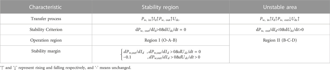
TABLE 4. Voltage stability characteristics of OWF.
4.2 Critical power calculation model
The extreme point of Pw, out-Id curve is the critical power injected at the DC side of the converter. The critical power can be obtained by dPw, out/dId = 0, as shown in (15):
The critical power under different cable parameters and reactive current can be drawn by (15), as shown in Figure 7.
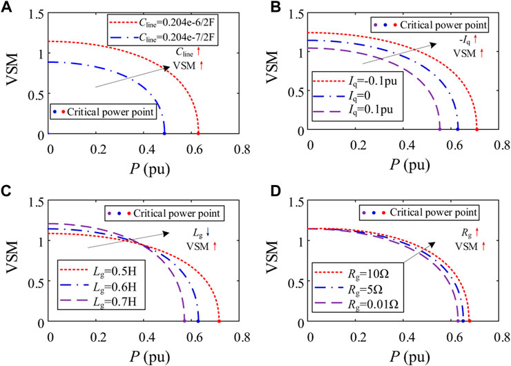
FIGURE 7. VSM curve under different parameters, (A) Cable capacitance parameters (Cline), (B) Output reactive current (Iq). (C) Grid inductance (Lg), (D) Grid resistance (Rg).
It can be seen from Figure 7 that as the output power increases, the VSM of the OWF decreases. When the VSM decreases to 0, the critical power under this state is reached. The influence of parameters on critical power is consistent with the results in Table 4. Compared with onshore WFs, the cable capacitance parameters of OWFs are larger, which increases the voltage stability margin of OWFs to a certain extent, but at the same time increases the risk of voltage exceeding the upper limit at low wind speeds. Therefore, reactive power compensation is required at low and high wind speeds, and the compensation direction (inductive or capacitive reactive power) is related to output power and grid impedance.
5 Experimental verification
5.1 Experimental platform
To verify the effectiveness of the proposed voltage characteristic modeling and criterion method of OWF, a simulation model of OWF is established based on the hardware in the loop platform composed of RT-LAB and digital signal processor (DSP), as shown in Figure 8. The topology and parameters of the OWF are shown in Figure A1 and Table 3. Among them, the circuit model of OWF is compiled in RT-LAB, and the voltage, current, power, and other signals of OWF are fed back to DSP through the I/O port. The control model of OWF is realized in DSP, which generates the driving signal of the OWF controller according to the RT-LAB feedback signal, thus forming the wind farm closed-loop control system.
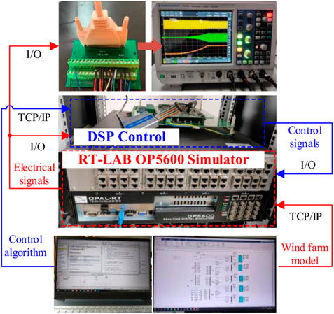
FIGURE 8. RT-LAB hardware in the loop experimental platform of OWF.
5.2 Analysis of experimental results
5.2.1 Voltage modeling and stability evaluation verification
To verify the accuracy of the OWF voltage modeling method and voltage stability evaluation model proposed in this paper, the following methods are used for comparison:
Method A: The voltage modeling method proposed in this paper considers submarine cable parameters and converter dynamics (shown in 12 and 15).
Method B: The traditional WF voltage modeling and evaluation methods are proposed in Kang et al. (2021), Huang and Wang (2018).
Method C: RT-LAB experimental results.
The grid impedance is set to 0.2H, the wind speed is increased from 3 m/s to 10.5 m/s at a rate of 2 m/s, and the rest of the parameters are the same as in Table 2. It can be seen that due to the reactive power consumption of grid impedance and submarine cable, the voltage at the PCC point continues to decrease as the output power increases.
Figure 9 shows the results of PCC voltage calculated by different methods. It can be seen that traditional methods (Method B) ignore cable parameters, resulting in a large deviation between calculation and experimental results (Method C), with the maximum deviation approaching 0.1 pu. The proposed method (Method A) is basically consistent with RT-LAB experimental results, which verifies the effectiveness of the proposed method.
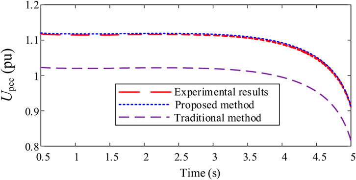
FIGURE 9. Comparison of different voltage models with experimental results.
Figure 10 shows the assessment results of voltage stability margin under different methods. As the capacitance parameters of submarine cables have a lifting effect on PCC voltage, and ignoring the cable capacitance parameters will lead to low assessment results. As shown in Figure 10, the limit power of Method B evaluation is 0.71 pu, with a deviation of 0.18pu compared with the experimental results. The method proposed in this paper is 0.897 pu, which is close to the experimental results, verifying the effectiveness of the proposed method.
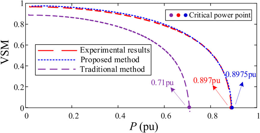
FIGURE 10. Comparison between different stability margin evaluation models and experimental results.
The internal voltage distribution of the OWF is shown in Figure 11. The grid impedance is set to 0.11H, and when the WT is half-loaded, Li-j represents the j-th WT on the i-th feeder. As the above theoretical analysis results are consistent, as the length of the feeder increases (the distance of the feeder is shown in Figure A1), the voltage amplitude increases continuously, and on the same feeder, the voltage of the WTs in the rear row is higher than that in the front row due to the effect of cable parameters. It can be seen that the PCC is the node with the lowest voltage in the entire wind farm, so the PCC is the weak point of the voltage of the OWF.
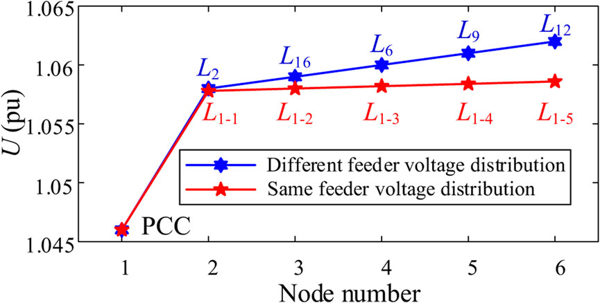
FIGURE 11. Comparison between different stability margin evaluation models and experimental results.
5.2.2 Verification of the influence of parameters on voltage stability
Case A. Different grid impedance.
The cable parameter settings are shown in Table 2. The Iq = 0 is set, the initial wind speed is 3 m/s, starting from 1.5s and rising to 10.5 m/s at the rate of 2 m/s. Figure 12A shows the experimental results when setting Lg = 0.11H, Rg = 0.01Ω (grid impedance). With the increase of output power, the voltage amplitude of PCC decreases from 1.065pu to 0.898pu. During the rise of output power, dPw,out/dId>0&dUdc/dt = 0, VSM decreases from 0.915 to 0.6687, but it always operates in the static voltage stability region of system (O-A-B region shown in Figure 6), and voltage instability does not occur.
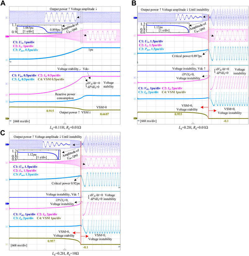
FIGURE 12. Comparison of VSM under different grid impedances, (A) Lg = 0.11H, Rg = 0.01Ω, (B) Lg = 0.2H, Rg = 0.01Ω, (C) Lg = 0.2H, Rg = 10Ω.
Figure 12B shows the experimental results when the grid impedance is set to Lg = 0.2H, Rg = 0.01Ω. As the output power increases, the voltage amplitude decreases continuously from the initial 1.12pu, and the system gradually moves along the O-A-B trajectory. When it reaches point B (dPw, out/dId = 0), reaches the critical power (0.897pu). When the injection power continues to increase, it is transferred to RegionII. At this time, dPw,out/dId<0&dUdc/dt>0, the voltage is unstable, VSM = −0.1, and the unbalanced power on the DC side tends to increase the DC voltage after the instability.
Figure 12C shows the experimental results when the grid impedance is set to Lg = 0.11H, Rg = 10Ω. As the output power increases, the system voltage instability occurs, and the critical power is 0.92pu, indicating that the grid resistance will increase the VSM.
Case B. Different submarine cable parameters.
The grid impedance setting is the same as Figure 12B. Figure 13A shows the experimental results when the cable capacitance parameter is set to CL = 0.204–7F/km, which is 10 times smaller than Figure 12B. At the initial moment, the voltage amplitude is 1.04 pu (lower than 1.12 pu in Figure 12B), the output power increases continuously, the voltage tends to be unstable, and the voltage amplitude decreases faster than Figure 12B, and the critical power is 0.814 pu, that is, the cable parameters raise the voltage, and when the cable capacity decreases, the critical power decreases (0.897 pu).
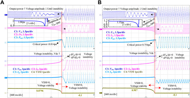
FIGURE 13. Comparison of VSM under different grid impedances. (A) RL = 0.0108 Ω/km, LL = 0.382e-3H/km, CL = 0.204–7F/km, (B) RL = 0.0108 Ω/km, LL = 0.382e-2H/km, CL = 0.204–6F/km.
Figure 13B shows the experimental results when the cable inductance parameter is set to LL = 0.382e-2H/km, Compared with Figure 12B, the inductance parameter is increased by 10 times, and the other parameter settings are the same. Initially, the voltage amplitude is 1.15pu, higher than Figure 12B, but with the increase of output power, the voltage amplitude decreases and the decline speed is faster than Figure 12B. When the critical power of 0.756 pu is reached, the voltage becomes unstable, that is, the increase of the cable inductance parameter makes the Upcc exceeding the upper limit more serious at low wind speed, and at the same time reduces the VSM at high wind speed.
The cable resistance parameter has the same effect as the grid resistance, and the influence trend is the same as that in Figure 12C, so it is not compared here.
Case C. Different output reactive power.
The cable parameters and grid impedance parameter settings are the same as in Figure 12A. Figure 14A shows the experimental results when Iq = −0.2pu is set. At the initial moment, the PCC voltage amplitude is 1.13pu. With the increase of output power, the voltage amplitude decreases to 1.02pu, which is higher than Figure 12A. In the process of power rise, VSM decreases from the initial 0.962 to 0.782, that is, it always operates in the O-A-B region, and the static voltage of the system is stable.
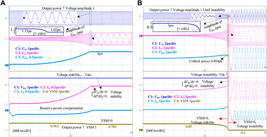
FIGURE 14. Comparison of VSM under different output reactive power. (A) Iq = 0.2pu, (B) Iq = −0.2pu.
Figure 14A shows the experimental results when Iq = 0.2 pu is set. Under the initial conditions, the PCC voltage amplitude is 1pu and VSM is 0.85, both lower than Figure 12A. With the increase of output power, the voltage amplitude decreases, and the voltage drop speed is faster than that in Figure 12A, until VSM = −0.1 voltage instability.
6 Conclusion
An OWF voltage modeling and stable area evaluation method that takes the submarine cable capacitance parameters and the DC dynamic characteristics of the converter into account is proposed in this paper. It can fully reflect the transfer process of the voltage instability of the OWF, and improve the evaluation accuracy of the voltage stability region. The following conclusions are drawn through theoretical analysis and experimental verification.
1) The voltage instability is represented by the DC charging characteristics caused by the imbalance of the input and output power at the DC side of the converter. The OWF is directly equivalent to the PQ node, which cannot directly reflect the power-voltage dynamic process of the OWF.
2) The capacitance parameter of submarine cable raises the system terminal voltage, which can improve the VSM, but it increases the risk of voltage exceeding the limit under low wind speed. The capacitance parameter of the cable increases 10 times from CL = 0.204–7F/km, the voltage rises 0.08pu, and the power limit increases 0.083pu.
3) The criterion method based on dPw, out/dId&dUdc/dt can accurately determine whether the system is in the static voltage stability area, and the relative distance between dPw, out/dId and 0 can quantitatively evaluate the static voltage stability level of the system.
In the future work, we will focus on the reactive power-voltage coordinated control strategy to improve the static voltage stability of OWFs, and establishing a small microgrid system with wind power converters to further verify the effectiveness of the proposed method.
Data availability statement
The original contributions presented in the study are included in the article/supplementary material, further inquiries can be directed to the corresponding author.
Author contributions
HT, HL substantial contribution to conception and design HT, HL substantial contribution to acquisition of data HT, RL substantial contribution to analysis and interpretation of data HT, ZZ drafting the article HT, RY critically revising the article for important intellectual content HT, RY, XZ final approval of the version to be published.
Funding
This work was supported by the National High-Tech ship research project, (No. MC-202025-S02), National Natural Science Foundationof China—State Grid Corporation Joint Fund for Smart Grid under Grant (No. U1966213).
Conflict of interest
The authors declare that the research was conducted in the absence of any commercial or financial relationships that could be construed as a potential conflict of interest.
Publisher’s note
All claims expressed in this article are solely those of the authors and do not necessarily represent those of their affiliated organizations, or those of the publisher, the editors and the reviewers. Any product that may be evaluated in this article, or claim that may be made by its manufacturer, is not guaranteed or endorsed by the publisher.
References
Cespedes, M., and Sun, J. (2014). Adaptive control of grid-connected inverters based on online grid impedance measurements. IEEE Trans. Sustain. Energy 5 (2), 516–523. doi:10.1109/TSTE.2013.2295201
Chen, K., and Han, J. (2020). “Influence of wind power grid connection on static voltage stability,” in 2020 7th International Forum on Electrical Engineering and Automation, Hefei, China, 25-27 September 2020 (IEEE), 371–374.
Du, X., Zhou, L., Guo, K., Yang, M., and Shao, N. (2015). Static voltage stability analysis of large-scale photovoltaic plants. China: Power System Technology.
Elliott, D., Bell, K. R. W., Finney, S. J., Adapa, R., Brozio, C., Yu, J., et al. (2016). A comparison of AC and HVDC options for the connection of offshore wind generation in great britain. IEEE Trans. Power Deliv. 31 (2), 798–809. doi:10.1109/TPWRD.2015.2453233
Guan, L., Yao, J., Liu, R., Sun, P., and Gou, S. (2021). Small-signal stability analysis and enhanced control strategy for VSC system during weak-grid asymmetric faults. IEEE Trans. Sustain. Energy 12 (4), 2074–2085. doi:10.1109/TSTE.2021.3079305
Guo, Y., Gao, H., Wu, Q., Zhao, H., Østergaard, J., and Shahidehpour, M. (2018). Enhanced voltage control of VSC-HVDC-Connected offshore wind farms based on model predictive control. IEEE Trans. Sustain. Energy 9 (1), 474–487. doi:10.1109/TSTE.2017.2743005
Gustavsen, B., and Mo, O. (2017). Variable transmission voltage for loss minimization in long offshore wind farm AC export cables. IEEE Trans. Power Deliv. 32 (3), 1422–1431. doi:10.1109/TPWRD.2016.2581879
Hou, X., Sun, Y., Han, H., Liu, Z., Yuan, W., and Su, M. (2019). A fully decentralized control of grid-connected cascaded inverters. IEEE Trans. Sustain. Energy 10 (1), 315–317. doi:10.1109/TPWRD.2018.2816813
Hu, X., Liang, J., Rogers, D. J., and Li, Y. (2013). Power flow and power reduction control using variable frequency of offshore AC grids. IEEE Trans. Power Syst. 28 (4), 3897–3905. doi:10.1109/TPWRS.2013.2257884
Huang, Y., and Wang, D. (2018). Effect of control-loops interactions on power stability limits of VSC integrated to AC system. IEEE Trans. Power Deliv. 33 (1), 301–310. doi:10.1109/TPWRD.2017.2740440
Kang, Y., Lin, X., Pan, C., and Liu, W. (2021). Analysis of power transmission characteristics of renewable energy grid-connected converter considering SVC and SVG compensation under weak grid condition. Proc. Chin. Soc. Electr. Eng. 41 (6), 2115–2124. doi:10.13334/j.0258-8013.pcsee.200514
Kang, Y., Lin, X., Zheng, Y., Quan, X., Hu, J., and Yuan, X. (2020). The static stable-limit and static stable-working zone for single-machine infinite-bus system of renewable-energy grid-connected converter. Proc. Chin. Soc. Electr. Eng. 40 (14), 4506–4515. doi:10.13334/j.0258-8013.pcsee.190906
Li, M., Zhang, X., Yang, Y., and Cao, P. (2018). International power electronics conference (IPEC-Niigata 2018 -ecce asia), 2973–2979.(Year)The grid impedance adaptation dual mode control strategy in weak grid
Musial, W., Spitsen, P., Duffy, P., Beiter, P., Marquis, M., Hammond, R., et al. (2022). Offshore wind market Report: 2022 edition. Golden, CO (United States): National Renewable Energy Lab.
Qi, B., Hasan, K. N., and Milanović, J. V. (2019). Identification of critical parameters affecting voltage and angular stability considering load-renewable generation correlations. IEEE Trans. Power Syst. 34 (4), 2859–2869. doi:10.1109/TPWRS.2019.2891840
Wang, L., Kuan, B. L., Yu, C. H., Wu, H. Y., Zeng, S. Y., Prokhorov, A. V., et al. (2019). Effects of submarine-cable types on performance of a future-scheduled offshore wind farm connected to taiwan power system. IEEE Ind. Appl. Soc. 56, 1171–1179. doi:10.1109/TIA.2020.2966159
Wu, D., Li, G., Javadi, M., Malyscheff, A. M., Hong, M., and Jiang, J. N. (2018). Assessing impact of renewable energy integration on system strength using site-dependent short circuit ratio. IEEE Trans. Sustain. Energy 9 (3), 1072–1080. doi:10.1109/TSTE.2017.2764871
Xin, H., Dong, W., Yuan, X., Gan, D., Wang, K., and Xie, H. (2016). Generalized short circuit ratio for multi power electronic based devices infeed to power systems. Proc. Chin. Soc. Electr. Eng. 36 (22), 6013–6027. doi:10.13334/j.0258-8013.pcsee.161682
Xu, Y., Mili, L., Korkali, M., Karra, K., Zheng, Z., and Chen, X. (2020). A data-driven nonparametric approach for probabilistic load-margin assessment considering wind power penetration. IEEE Trans. Power Syst. 35 (6), 4756–4768. doi:10.1109/TPWRS.2020.2987900
Zhao, H., Wu, Q., Guo, Q., Sun, H., Huang, S., and Xue, Y. (2016). Coordinated voltage control of a wind farm based on model predictive control. IEEE Trans. Sustain. Energy 7 (4), 1440–1451. doi:10.1109/TSTE.2016.2555398
Appendix A: The topology and feeder distance of H3 FWF.
The derivation process of UPCC is as follows. The real part and imaginary part on both sides of (10) are equal, that is, the imaginary part on the right side of the equation is 0.
Square both sides of (A1) at the same time to get:
Suppose the coefficient of the real part Ug in the Upcc is acosθpcc + bsinθpcc = M, and square it to get:
Further, the variable M can be expressed as:
Substitute the expression of variable M into (10) to get:
The topology and feeder distance of H3 OWF are shown in Figure A1.
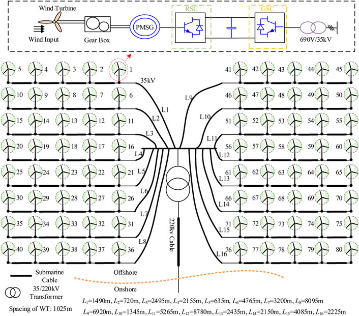
FIGURE A1. The topology and feeder distance of H3 FWF.
Keywords: voltage stability, cable capacitance, offshore wind farms, stability criterion, converter
Citation: Tan H, Li H, Yao R, Liu R, Zhou Z and Zhang X (2023) Static voltage stability analysis and evaluation of vector controlled offshore wind farm considering cable capacitance parameters. Front. Energy Res. 11:1116090. doi: 10.3389/fenrg.2023.1116090
Received: 05 December 2022; Accepted: 03 January 2023;
Published: 19 January 2023.
Edited by:
Joshuva Arockia Dhanraj, Hindustan University, IndiaReviewed by:
Pavan Kalyan Lingampally, Hindustan University, IndiaAnitha Gopalan, Saveetha University, India
Copyright © 2023 Tan, Li, Yao, Liu, Zhou and Zhang. This is an open-access article distributed under the terms of the Creative Commons Attribution License (CC BY). The use, distribution or reproduction in other forums is permitted, provided the original author(s) and the copyright owner(s) are credited and that the original publication in this journal is cited, in accordance with accepted academic practice. No use, distribution or reproduction is permitted which does not comply with these terms.
*Correspondence: Hui Li, Y3F1bGhAMTYzLmNvbQ==; Ran Yao, eWFvcmFuMTIzNEAxNjMuY29t