Short-term load forecasting based on CEEMDAN-FE-ISSA-LightGBM model

To address the problems of low load forecasting accuracy due to the strong non-stationarity of electric loads, this paper proposes a short-term load forecasting method based on a combination of the complete ensemble empirical modal decomposition adaptive noise method-fuzzy entropy (CEEMDAN-FE) and the Light Gradient Boosting Machine (LightGBM) optimized by the improved sparrow search algorithm (ISSA). First, the original data are decomposed by the complete ensemble empirical modal decomposition adaptive noise algorithm to obtain the eigenmodal components (IMFs) and residual values. Second, the obtained sequences are entropy reorganized by fuzzy entropy, and thus new sequences are obtained. Third, the new sequences are input into the improved sparrow search algorithm-Light Gradient Boosting Machine model for training and prediction. The improved sparrow search algorithm algorithm can realize parameter optimization of the Light Gradient Boosting Machine model to make the data match the model better, and the predicted values of each grouping of the model output are superimposed to obtain the final predicted values. Finally, the effect is compared by the error function, and the comparison results are used to test the performance of the algorithm. The experiments showed that the smallest evaluation metrics were obtained in Case 1 (MAE = 32.251, MAPE = 0.0114,RMSE = 42.386, R2 = 0.997) and Case2 (MAE = 3.866, MAPE = 0.003, RMSE = 5.940, R2 = 0.997).

1 Introduction

Short-term load forecasting is related to the safe and economic operation and stable development of power systems, and is an important part of the operational planning of power grids (Hassan et al., 2016; Gong. et al., 2021). With the widespread use of distributed energy sources and power electronic devices, the behavior of short-term electric loads has become more and more com-plex, which brings great challenges to load forecasting methods, and it is of great significance to accurately perform load forecasting to improve socioeconomic efficiency (Chen et al., 2018; Lv et al., 2022; Blake et al., 2021).

Currently, the methods for short-term load forecasting include two main categories: mathematical methods and machine learning methods (Ge et al., 2021). For the former, the advantages are simple models, small computational effort, and fast forecasting, such as multiple linear regression (Kim et al., 2018), gray correlation models (Guo et al., 2022), and ARIMA (Wei and Zhen-gang, 2009). The models developed by this type of methods depend on the assumptions of data distribution and the rationality of the model. It is difficult to meet the conditions needed for them because of the non-smoothness and randomness of the electric load. Machine learning methods mainly include artificial neural networks (Goh et al., 2021), support vector machines (Liu et al., 2018), and decision tree models (Song et al., 2021), which can better deal with non-linear problems, especially decision tree models, which have unique advantages in solving prediction problems. The literature (Yao et al., 2022) achieved power prediction of electric loads based on the LightGBM algorithm to screen features and make predictions. However, due to the large number of parameters involved, the model needs to be reasonably tuned before it can perform better. Despite the advantages of machine learning, it is still difficult to take into account the variation of features on different time scales, especially when the time-series features are complex. There-fore, the idea of attenuating the non-smoothness and randomness of the data and processing them by machine learning on this basis has become a consensus. The literature (Baniamerian et al., 2009) used orthogonal wavelet decomposition of electric load data to eliminate its volatility, and then modeled the prediction of the decomposed signal to improve the stability and accuracy of the prediction. The above decomposition methods require the selection of suitable basis functions to be most effective, and the reasonable selection of basic functions is difficult. In contrast, empirical modal decomposition (EMD) can decompose the data based on its timing characteristics, and does not rely on artificially set basis functions. Theoretically, EMD can handle any type of time series (Zheng et al., 2017). The literature (Fan et al., 2020) describes the application of EMD algorithm in load forecasting, which is prone to “modal confusion” and affects the efficiency of the decomposition. For the problem of “modal overlap,” the complete ensemble EMD with adaptive noise (CEEMDAN) mentioned in (Chen et al., 2021) can reduce the error in the signal reconstruction process and solve the “modal overlap” caused by adding noise to the signal. It can reduce the error in the signal reconstruction process and solve the problem of “mode overlap” caused by the addition of noise, better reflect the characteristics of each frequency load, and accurately portray the load demand of the re-search object. The decomposition algorithm can better predict the load information, but when the number of sequences obtained is large, it may lead to too much operation and reduce the efficiency of operation.

In order to effectively deal with the non-smoothness problem of electricity load forecasting and improve the efficiency and accuracy of short-term load forecasting. In this paper, a prediction model based on the combination of CEEMDAN-FE algorithm and ISSA-LightGBM algorithm is proposed. The original data is processed by the CEEMDAN-FE algorithm, and the CEEMDNA algorithm decomposes the non-stationary electricity load data into different IMFs with corresponding frequencies. Next, the complexity of each IMF is calculated by the FE algorithm, and the IMFs with similar fuzzy entropy values are recombined to obtain a new set of sequences. This method can effectively improve the computational efficiency and solve the problems of over-decomposition and computational burden. In order to obtain better prediction results, it is necessary to debug the parameters in the LightGBM model. In order to improve the debugging efficiency and make the data and model more compatible, this paper improves the SSA algorithm to overcome the problem that it easily falls into local convergence and obtains the ISSA algorithm with stronger global search capability, which can better This paper improves the SSSA algorithm to overcome its tendency to fall into local convergence, and obtains the ISSA algorithm with better global search capability, which can better complete the tuning work. The parameters of the LightGBM model are optimized by the ISSA algorithm, and then the prediction results of each new sequence are obtained, and finally the prediction results of each part are superimposed and output.

The contributions of this paper are summarized as follows:

• This paper proposes a load forecasting model based on the idea of “decomposition-reconstruction-combination.” In order to avoid the computational burden caused by the over-decomposition of the CEEMDAN algorithm, the fuzzy entropy value after the initial decomposition is calculated and used as the basis for reconstruction to obtain a new series. Finally, a prediction model is built for each smoother subsequence after reconstruction, and the output results are superimposed to obtain accurate prediction results.

• The ISSA-LightGBM prediction model is proposed. The tuning parameter of LightGBM involves several parameters, while around different components, the parameters are different, and this paper seeks the parameters with the help of an algorithm; ISSA is obtained by improving the SSA algorithm, which improves its global convergence ability, and can better find the suitable parameters to make the data match with the model and improve the accuracy of prediction.

The rest of the paper is organized as follows. Section 2 presents the CEEMDAN-FE algorithm, which reduces the non-smoothness of the data and improves the prediction efficiency. Section 3 introduces the prediction method used in this paper and the improved heuristic algorithm for tuning the reference. Section 4 presents the overall structure of the proposed algorithm. Section 5 presents a case study and Section 6 draws conclusion.

2 CEEMDAN-FE

2.1 Complete ensemble empirical mode decomposition adaptive noise methed

The CEEMDAN algorithm is an improvement of the empirical modal algorithm by the researchers of (Torres, 2011). This algorithm can decompose the data according to the actual data situation and temporal characteristics, and divide them into several eigenmodal components (IMF) and residuals (Res) according to the instantaneous frequency, and the resulting components have stronger regularity compared to the original data. The decomposition method of CEEMDAN consists of several steps as follows.

1) The Gaussian white noise with a mean value of 0 is weighted and added to the original time-series data x(t) to obtain the preprocessing sequence x_i(t) for n experiments (i = 1, 2, ......, n).

$\begin{array}{c}{x}_i\left(t\right)=x\left(t\right)+\lambda {\delta }_i\left(t\right)\end{array}(1)$

2) The EMD decomposition of x_i(t) is performed and the decomposition yields the first component $\overline{IM{F}_1\left(t\right)}$,

$\begin{array}{c}\overline{IM{F}_1\left(t\right)}=\frac{1}{n}{\displaystyle \sum }_{i=1}^{n}IM{F}_1^i\left(T\right)\end{array}(2)$

The first residual signal r₁(t) is calculated as

$\begin{array}{c}{r}_1\left(t\right)=x\left(t\right)-\overline{IM{F}_1\left(t\right)}\end{array}(3)$

3) Repeat the above operation for the decomposed residual sequence to obtain the second modal component,

$\begin{array}{c}\overline{IM{F}_2\left(t\right)}=\frac{1}{n}{\displaystyle \sum }_{i=1}^n{E}_1\left(r_1\left(t\right)+{\epsilon }_1{E}_1\left({\omega }^i\left(t\right)\right)\right)\end{array}(4)$

4) Performing the above operation for each of the remaining stages, the j th residual signal is calculated:

$\begin{array}{c}{r}_j\left(t\right)=r_{j-1}\left(t\right)-IM{F}_j\left(t\right)\end{array}(5)$

Repeat the calculation process of the previous step (3) to obtain the j+1 th modal component as,

$\begin{array}{c}\overline{IM{F}_{j+1}\left(t\right)}=\frac{1}{n}{\displaystyle \sum }_{j=1}^n{E}_1\left(r_j\left(t\right)+{\epsilon }_j{E}_j\left({\omega }^i\left(t\right)\right)\right)\end{array}(6)$

5) Repeat the above step (4) until the number of extreme value points of the residual components satisfies the corresponding condition and the decomposition cannot be continued, then the CEEMDAN decomposition is finished. At this time, the original data is decomposed into J IMFs components and residual components.

$\begin{array}{c}R\left(t\right)=x\left(t\right)-{\displaystyle \sum }_{j=1}^J\overline{IM{F}_j\left(t\right)}\end{array}(7)$

Finally, the raw load data are decomposed as follows:

$\begin{array}{c}x\left(t\right)={\displaystyle \sum }_{j=1}^J\overline{IM{F}_j\left(t\right)}+R\left(t\right)\end{array}(8)$

2.2 Fuzzy entropy

Fuzzy entropy is used as a measure of time series complexity, and its exponential function is introduced to solve the similarity measure while spatial reconstruction, so that the fuzzy entropy value can change steadily with the parameters. The larger the fuzzy entropy value is, the more complex its time series complexity is. Its basic process is as follows.

1) Recombination of sequence y

$\left.a^n\left[i\right]=\{y\left(i\right),y\left(i+1\right),\dots y\left(i+n-1\right)\}-y_0\left(i\right)\right\}(9)$

where n represent phase space dimension; i = 1,2, …,M-n+1.

$\begin{array}{c}{a}_0\left(i\right)=\frac{1}{m}{\displaystyle \sum }_{j=1}^{m-1}a\left(i+j\right)\end{array}(10)$

2) Introduction of fuzzy affiliation function

$\begin{array}{c}{H}_{ij}^n=\exp \left(-In\left(2\right)\ast {\left(\frac{c_{ij}^m}{r}\right)}^2\right)\end{array}(11)$

where r represents the similarity tolerance limit.

3) The $c_{ij}^n$ is given follows:

$\begin{array}{c}{c}_{ij}^n=c\left[a^n\left[i\right],s^n\left[j\right]\right]=\underset{p=\mathrm{1,2},\cdots ,m}{\max }\left(\left|a\left(i+p-1\right)-a_0\left(i\right)\right|-\left|a\left(j+p-1\right)-a_0\left(j\right)\right|\right)\end{array}(12)$

4) The formula $D_i^n\left(r\right)$ is given as follows:

$\begin{array}{c}{D}_i^n\left(r\right)={\left(M-n\right)}^{-1}{\displaystyle \sum }_{j=1,j\ne i}^{M-n+1}{H}_{ij}^n\end{array}(13)$

where M represents time series length.

5) Define the function

$\begin{array}{c}{\varphi }^m\left(r\right)={\left(M-n+1\right)}^{-1}{\displaystyle \sum }_{i=1}^{M-n+1}{D}_i^n\left(r\right)\end{array}(14)$

6) When M is a finite value, the calculated value of FE is

$\begin{array}{c}FE\left(n,r,M\right)=In{\varphi }^n\left(r\right)-In{\varphi }^{n+1}\left(r\right)\end{array}(15)$

3 LightGBM based on ISSA optimization

3.1 Improvement of the sparrow search algorithm

3.1.1 Standard sparrow search algorithm

The sparrow search algorithm is a novel metaheuristic algorithm proposed by Xue and Chen (Wu and Wang, 2021), which is based on the imitation of the foraging and anti-predatory behaviors of sparrow populations. The basic idea is to calculate the fitness of individual spar-rows by constructing fitness functions, and then realize the state transformation between individuals, which effectively avoids falling into local optimum. Compared with the traditional swarm optimization algorithm, this algorithm has better foraging ability, con-vergence, and robustness. The principle is as follows.

Assume that the population consisting of m sparrows is depicted as Eq. 16

$\begin{array}{c}X=\left[\begin{array}{ccc}{x}_1^1& \cdots & x_1^d\\ ⋮& \ddots & ⋮\\ x_m^1& \cdots & x_m^d\end{array}\right]\end{array}(16)$

In Eq. 16, X is the randomly generated sparrow population; x is each sparrow; d is the number of dimensions of the population, which is the same as the number of parameters to be optimized in the LightGBM model; and m is the number of sparrows.

$\begin{array}{c}{G}_x=\left[\begin{array}{c}g\left(\left[x_1^1{x}_1^2\cdots x_1^d\right]\right)\\ g\left(\left[x_2^1{x}_2^2\cdots x_2^d\right]\right)\\ ⋮\\ g\left(\left[x_m^1{x}_m^2\cdots x_m^d\right]\right)\end{array}\right]\end{array}(17)$

where G_x is the fitness function matrix; g denotes the fitness of the individuals. The population size will change according to the change of adaptation value, and the whole will be more adapted to the change in the environment. In this process, there will be some individuals in the population with higher adaptation values, and these individuals will have priority in the search process to obtain prey. In the iterative process, its position is updated as,

$\begin{array}{c}{X}_{i,j}^t=\left\{\begin{array}{c}{X}_{i,j}^t\ast \exp \left(-\frac{i}{\alpha \ast ite{r}_{\mathit{max}}}\right),R_2<ST\\ X_{i,j}^t+Q\ast L,R_2\ge ST\end{array}\right.\end{array}(18)$

where t is the number of iterations of the population, X_i,j is the information of the i th sparrow at the j th dimension, and iter_max is the maximum value of the number of iterations.

The position update of the joiner, denoted as

$\begin{array}{c}{X}_{i,j}^{t+1}=\left\{\begin{array}{c}Q\ast \exp \left(-\frac{X_{worst}^t-X_{i,j}^t}{i^2}\right),i>\frac{n}{2}\\ X_p^{t+1}+\left|X_{i,j}^t-X_p^{t+1}\right|,i\le \frac{n}{2}\end{array}\right.\end{array}(19)$

where X_p is the optimal position occupied by the discoverer in the sparrow population at this time, and X_worst is the global worst position of the individuals in the current population.

When the proportion of individuals aware of danger reaches 10%–20% of the overall population size, the population feels the danger and engages in anti-predation, the mathematical expression is given as,

$\begin{array}{c}{X}_{i,j}^{t+1}=\left\{\begin{array}{c}{X}_{best}^t+\mathrm{\beta }\left|X_{i,j}^t-X_{best}^t\right|,f_i>f_g\\ X_{i,j}^t+K\left[\frac{X_{i,j}^t-X_{best}^t}{\left(f_i-f_w\right)+\epsilon }\right],f_i=f_g\end{array}\right.\end{array}(20)$

where X_best is the current global optimal position, β is the control parameter of the step size and obeys N (0, 1) distribution. k∈[-1,1]. f_i is the fitness value of the i th individual, f_g is the global best value in the current situation of the population, f_w is the global worst value in the current situation of the population, and ε is a constant.

3.1.2 Improving the sparrow search algorithm

To address the problems that the sparrow search algorithm suffers from decreasing population diversity near the global optimal solution and easily falls into the local optimum, this paper improves the global search capability by initializing the population with Sinusoidal chaotic mapping; the tangent flight strategy is used to perturb the optimal solution to ensure the diversity of spatial search and improve the convergence accuracy.

Since the values of each individual in each dimension are randomly generated in the initialization stage, the initial solutions are prone to aggregation, resulting in low coverage of the initial solutions in the solution space and insignificant differences between individuals, while Sinusoidal chaos mapping initialized population can solve this problem well, and the random solutions generated by it are stable and have high coverage. Its expression is shown,

$\begin{array}{c}{X}_{k+1}=a\ast X_k^2\sin \left(\pi X_k\right)\end{array}(21)$

Sinusoidal chaotic mappings are more uniformly distributed in the search space, so that the solutions are uniformly distributed in the feasible domain, which can speed up the global search and increase the convergence speed.

The sparrow search algorithm converges to the current solution by jumping directly to the optimal solution instead of moving toward the optimal solution like the traditional algorithm, which also leads to the algorithm easily falling into the local optimum. To reduce the impact of the decreasing population diversity in the search process at the later iteration, the tangential search algorithm (TSA) is borrowed here, which moves in large steps through the tangential flight The characteristics of the sparrow search algorithm are modified for the search foraging mechanism.

A stepwise method based on a tangent function, called a tangent flight, is employed in the TSA algorithm, which helps to explore space. The combined global and wandering exploration equation is shown,

$\begin{array}{c}{X}^{t+1}=X^t+step\ast \tan \left(\theta \right)\end{array}(22)$

From the above equation, when θ is closer to π/2, the larger the cut value is, the farther the obtained solution is from the current solution; when θ is close to 0, the smaller the cut value is, the closer the obtained solution is to the current solution. Using this formula to correct the new update value obtained from the position update formula, the improvement can search a larger space locally compared to the update strategy of the original algorithm.

The algorithm flow is:

1) Set the number of update iterations for the population, adjust the respective proportions of joiners and predators after initialization, and determine the parameter information group objects to be optimized, i.e. each individual, and the fitness value objects;

2) Calculate the fitness value and rank them according to the fitness value;

3) Predator location update;

4) Update joiner location;

5) Updated Vigilantes location;

6) Determining the latest position of the sparrow and the optimal fitness value;

7) A tangential flight strategy perturbs the latest position to improve the global search capability and avoid getting stuck in a local optimum;

8) Determine if the previous predetermined requirements have been met, if so finish, otherwise continue to repeat Step2) - 7).

The overall structure of the improved sparrow search algorithm is shown in Figure 1, and the detailed steps are as follows.

FIGURE 1

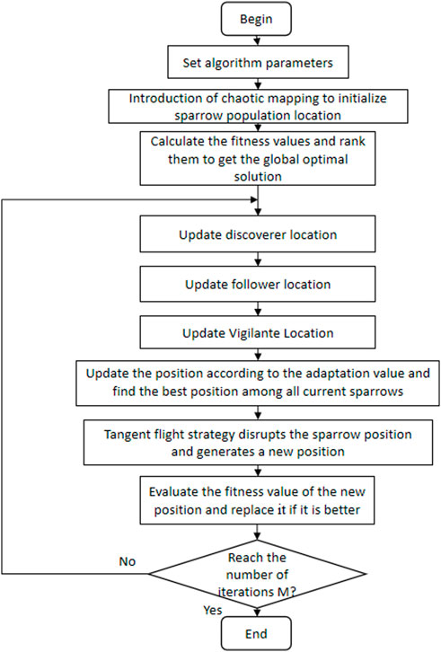
FIGURE 1. ISSA algorithm structure.

3.1.3 Validation of the effect of an improved sparrow search algorithm

To visualize the overall performance of the improved sparrow algorithm, the particle swarm (PSO) algorithm, gray wolf (GWO) algorithm, sparrow search (SSA) algorithm, and the proposed algorithm are used for comparison, respectively. The parameters of the comparison experiment are set as follows: the number of populations is 20, and the number of iterations is 100. The measurement function and related parameters are shown in Table 1 and Eq. 23.

$\begin{array}{c}\left\{\begin{array}{c}{f}_1={\displaystyle \sum }_{i=1}^n{x}_i^2\\ f_2={\displaystyle \sum }_{i=1}^n\left[x_i^2-10\cos \left(2\pi x_i\right)+10\right]\\ f_3=-20\exp \left(-0.2\sqrt{\frac{1}{n}{\displaystyle \sum }_{i=1}^n{x}_i^2}\right)-\exp \left(\frac{1}{n}{\displaystyle \sum }_{i=1}^n\left(2\pi x_i\right)\right)+20+e\end{array}\right.\end{array}(23)$

TABLE 1

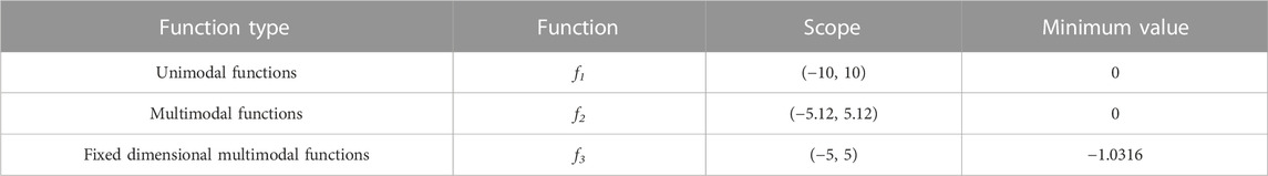
TABLE 1. Test functions and their related parameters.

From Table 2, we can see that ISSA has the best overall performance, followed by SSA and GWO, while PSO has the least satisfactory effect. The adaptation curves of the two functions after intercepting are shown in Figure 2.

TABLE 2

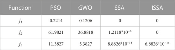
TABLE 2. Performance comparison of each algorithm.

FIGURE 2

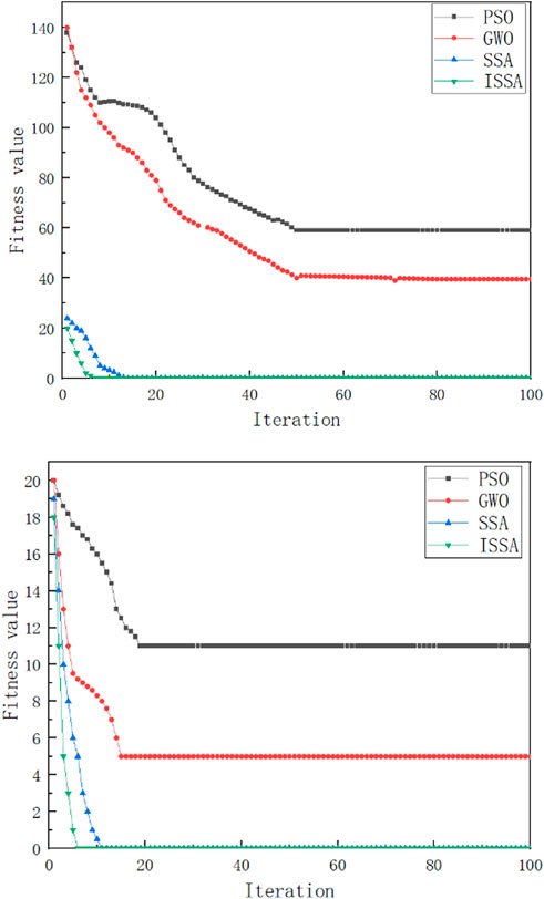
FIGURE 2. 100 iterations of the curve.

3.2 LightGBM

LightGBM is an integrated learning model based on the Distributed Gradient Boosting Decision Tree (GBDT) (Choi and Hur, 2020). The algorithm uses a decision tree as the base learner, which can be represented as.

$\begin{array}{c}{H}_T\left(x\right)={\displaystyle \sum }_{t=1}^T{H}_t\left(x\right),H_t\in \theta \end{array}(24)$

where, H_t is the t th learner; Θ is the set space of all learners.

LightGBM improves the performance of the model by multiple iterations, and the mapping function from the input space to the gradient space G is obtained by a learner. Given a training set {x₁,...,x_n} with a data volume of n, where x_i is a vector of dimension i of space X_s with s. When the learner obtained in the previous iteration is H_t-1(x) and the loss function is L(y, H_t-1(x)), the goal of the current iteration is to find the weak learner h_t(x) such that the loss function in the current round is minimized, i.e.,

$\begin{array}{c}{h}_t\left(x\right)=\mathit{arg}\underset{h\in H}{\min }L\left(y,H_{t-1}\left(x\right)+h_t\left(x\right)\right)\end{array}(25)$

The negative gradient of this loss function is calculated and used to obtain an ap-proximation of the loss function for this round, which can be expressed as

$\begin{array}{c}{r}_t=-\frac{\partial L\left(y,H_{t-1}\left(x\right)\right)}{\partial H_{t-1}\left(x\right)}\end{array}(26)$

The objective function is usually quadratic, and h_t(x) can be approximated as

$\begin{array}{c}{h}_t\left(x\right)=\mathit{arg}\underset{h\in H}{\min }\sum {\left(r_t-h_t\left(x\right)\right)}^2\end{array}(27)$

The final strong learners obtained for this iteration:

$\begin{array}{c}{H}_t\left(x\right)=H_{t-1}\left(x\right)+h_t\left(x\right)\end{array}(28)$

The hyperparameters involved in the LightGBM model constructed in this paper mainly include: the number of weak classifier K, the complexity of generating decision trees d, the learning rate lr, and the number of leaf nodes. They are optimized by the ISSA algorithm, and the objective function of the optimization algorithm is the mean squared difference between the predicted and true values, and the solution steps are as follows.

1) Initialisation: The ISSA algorithm is initialized by determining the size of the sparrow population, the number of iterations and the safety threshold based on the constrained range of variables.

2) Adaptive values: The error information between the predicted and sample data from the LightGBM model is used to determine the adaptive value for each sparrow, and this paper uses the root mean square between the predicted and true values as the adaptive value.

3) Update: Update the position and information of individual sparrows in the population, i.e., hyperparameters. After obtaining the location and information update, the new fitness value for each individual will be obtained by validating the LightGBM prediction model with this hyperparameter premise and saving the best value of individual location and global location in the population, i.e. the best hyperparameter information in this round.

4) Iteration: Determine if the current state satisfies the end condition set by the algorithm. If the condition is met, we exit the loop and output the optimal individual solution, which is the optimal parameter for the test model; if not, we continue the loop step 3).

5) Output result: If the set condition is satisfied, the best hyperparameter value is output as the parameter of the LightGBM prediction model for that sequence, and the prediction result is also obtained.

The overall structure of the prediction model is shown in Figure 3.

FIGURE 3

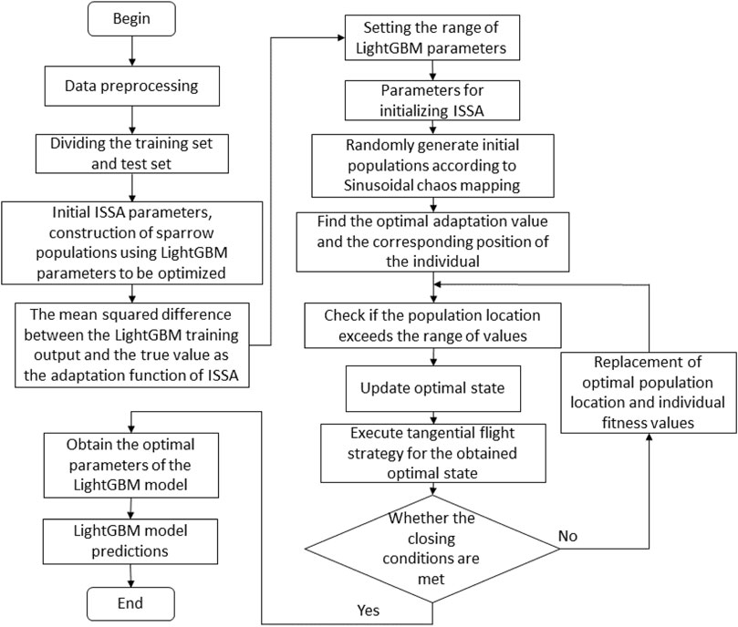
FIGURE 3. ISSA-LightGBM algorithm structure.

4 Construction of CEEMDAN-FE-ISSA-LightGBM for short-term load forecasting

In order to effectively deal with the non-smooth problem of electricity load forecasting and improve the efficiency and accuracy of short-term load forecasting. In this paper, a “decomposition-reconstruction-combination” load forecasting model based on the combination of the CEEMDAN-FE algorithm and the ISSA-LightGBM algorithm is proposed. Next, the complexity of each IMF is calculated by the FE algorithm, and IMFs with similar fuzzy entropy values are recombined to obtain a new set of sequences. This method can effectively improve the computational efficiency and solve the problems of over-decomposition and computational burden. In order to obtain better prediction results, it is necessary to debug the parameters in the LightGBM model. In order to improve the debugging efficiency and make the data and model more compatible, this paper improves the SSA algorithm, overcomes the problem that the SSA algorithm is easy to fall into local convergence, and obtains the ISSA algorithm with better global search capability. The parameters of the LightGBM model are optimised by the ISSA algorithm, then the prediction results of each new sequence are obtained, and finally the prediction results of each part are superimposed and output.

1) The non-stationary and random nature of the load data affect the accuracy of the forecasting. The raw load data are decomposed by CEEMDAN to obtain more stationary eigenmodal components and residual values.

2) The obtained components are subjected to a fuzzy entropy operation to obtain the entropy value of each component, and a new set of IMF components is obtained by reorganising them according to the entropy value, thus avoiding the computational burden problem caused by over-decomposition and thus improving the efficiency of the operation.

3) Input the obtained new components into ISSA-LightGBM for prediction

4) As different sub-sequences have different characteristics, a single model cannot accommodate all the characteristics of each subsequence. For this reason, an ISSA-LightGBM model with different hyperparameters is proposed to predict sub-sequences with different characteristics. In a practical problem, the model is optimised by the ISSA algorithm to optimise the hyperparameters of LightGBM, trade-offs are made between learning performance and model complexity, and the corresponding prediction model is obtained for each subsequence characteristic and predicted one by one.

5) The results of the components obtained in step 3) are superimposed to obtain the final prediction value.

The structure of the proposed prediction model in this paper is shown in Figure 4.

FIGURE 4

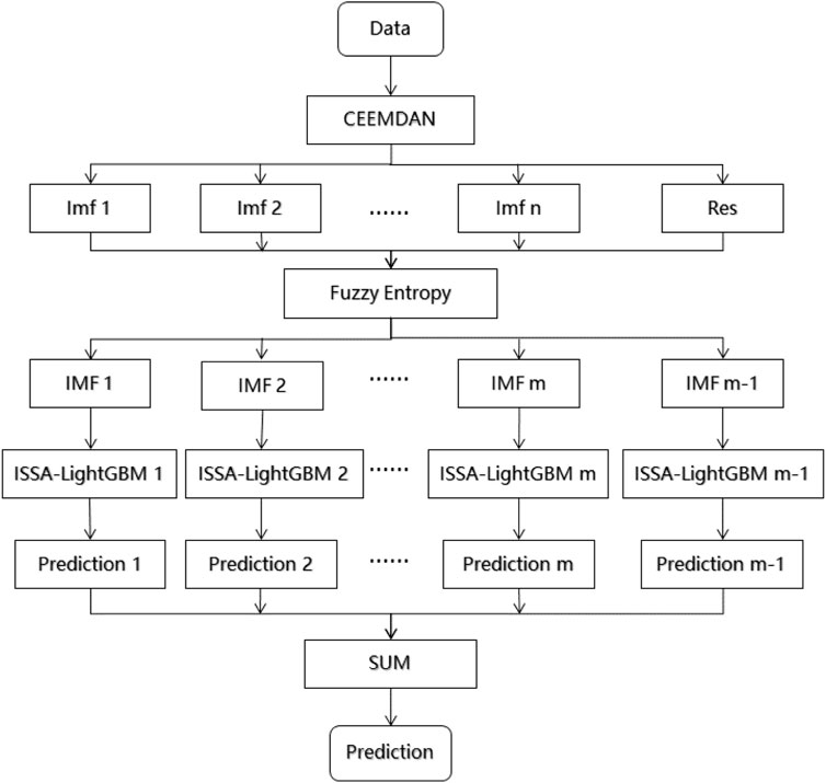
FIGURE 4. CEEMDAN-FE-ISSA-LightGBM model structure.

5 Case study

5.1 Data description

To verify the validity of the short-term load forecasting model proposed in this paper, two short-term time scales are used for validation in this paper. Case 1 uses the electricity load data of a region in China from January 1 to 31 December 2014 as the experimental data set, with 1 h as the sampling interval and a total of 8,760 sampling points, where the ratio of the training set to the test set is 8:2, and selects the data from December 28 to 31 for empirical validation. Case 2 uses the average electricity load consumption of a city in China from 21 July 2015 to 23 January 2020 as the experimental dataset, with a sampling interval of 1 day and a total of 1,667 sampling points, where the ratio of the training set to the test set is also 8:2, and the latter 100 days are selected for demonstration. GBDT, LSTM, LightGBM, CEEMDAN-GBDT, CEEMTAN-LSTM, CEEMDAN-LightGBM, SEEMDAN-FE LightGBM and the algorithm mentioned in this paper, CEEMDAN FE ISSA LightGBM, were compared.

5.2 Predictive model evaluation metrics

To better evaluate the proposed prediction algorithm and to compare it with the pre-diction accuracy of the comparison algorithm, the evaluation metrics used in this calculation are mean absolute error (MAE), mean absolute percentage error (MAPE) and root mean square error (RMSE).

$\begin{array}{c}MAE=\frac{1}{n}{\displaystyle \sum }_{i=1}^n\left|y_i-{\widehat{y}}_i\right|\end{array}(29)$

$\begin{array}{c}MAPE=\frac{100\%}{n}{\displaystyle \sum }_{i=1}^n\frac{\left|y_i-{\widehat{y}}_i\right|}{y_i}\end{array}(30)$

$\begin{array}{c}RMSE=\sqrt{\frac{1}{n}{\displaystyle \sum }_{i=1}^n{\left(y_i-{\widehat{y}}_i\right)}^2}\end{array}(31)$

$\begin{array}{c}{R}^2=1-\frac{{\sum }_{i=1}^n{\left(y_i-{\widehat{y}}_i\right)}^2}{{\sum }_{i=1}^n{\left(\overline{{\widehat{y}}_i}-{\widehat{y}}_i\right)}^2}\end{array}(32)$

In this formula, n is the number of prediction points, and are the true and predicted values obtained at the i th predicted time point in the test set, respectively.

5.3 Case study

5.3.1 Case study 1:1-h time-scale load forecasting

5.3.1.1 Experimental CEEMDAN-FE decomposition of raw load information

From Figure 5, we can find that the first set of data itself has strong non-smoothness and randomness, which is difficult to predict directly, so here the original load data is decomposed by CEEMDAN algorithm to reduce its non-smoothness and randomness.

FIGURE 5

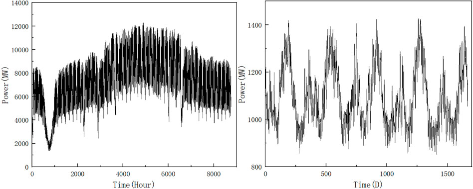
FIGURE 5. Raw load data.

The decomposed load data are shown in Figure 6. It can be seen that the regularity of the processed data is more obvious, and the fluctuations are less drastic and have significant time-series characteristics.

FIGURE 6

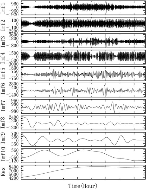
FIGURE 6. Results of the decomposition of Case 1 CEEMDAN.

To further improve the prediction efficiency, reduce the scale of the prediction model operation, and reduce the time used for prediction. The decomposed sequence is processed by the fuzzy entropy algorithm, and the original sequence is reorganized according to its entropy value to obtain a new sequence with less quantity than the decomposed quantity. The fuzzy entropy value of the decomposed quantity is solved as shown in Figure 7.

FIGURE 7

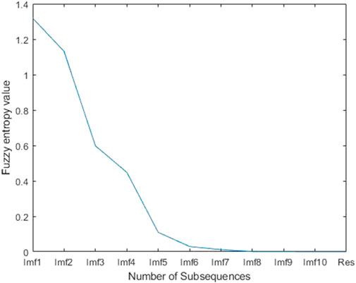
FIGURE 7. Fuzzy entropy analysis of the decomposition results of Case 1.

From Figure 7, it can be seen that the fuzzy entropy values of Imf8-Res are similar and can be recombined into a new sequence, and the recombined components are shown in Table 3.

TABLE 3

TABLE 3. Recombination of each sequence.

The decomposition results obtained after recombination are shown in Figure 8.

FIGURE 8

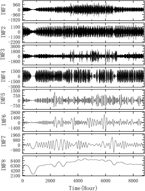
FIGURE 8. CEEMDAN-FE processing results of Case 1.

5.3.1.2 Prediction experiments based on the CEEMDAN-FE-ISSA-LightGBM algorithm

To verify the effectiveness of the proposed model, the original load data were first processed using the CEEMDAN-FE algorithm, and the new sequences were obtained and input into the ISSA-LightGBM model for prediction respectively, and the group prediction results were summed to obtain the complete prediction results. Here, the number of populations of the algorithm is set as 30, the proportion of discoverers, joiners, and vigilantes in the population is 7:2:1, and the number of iterations is 100, where the prediction results are shown in Figure 9.

FIGURE 9

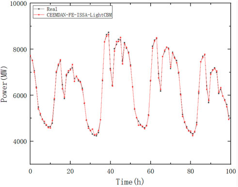
FIGURE 9. Prediction results of Case 1.

The CEEMDAN FE ISSA LightGBM algorithm was compared with other models, where the GBDT model has 50 learners, a learning rate of 0.1, a maximum depth of 12 for the decision tree, and 40 leaf nodes. The LightGBM model parameters were similar to those of GBDT, and the same number of parameters was used for the single model comparison. The LSTM model has 24 neurons and 100 epochs, and the results are shown in Figures 11, 12. The comparison results are shown in Figures 10, 11.

FIGURE 10

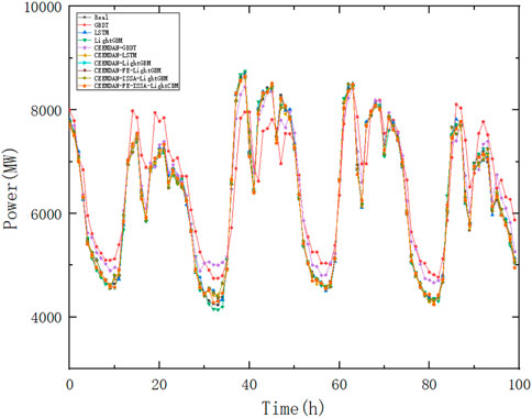
FIGURE 10. Case 1 graph of this paper’s model versus a single model.

FIGURE 11

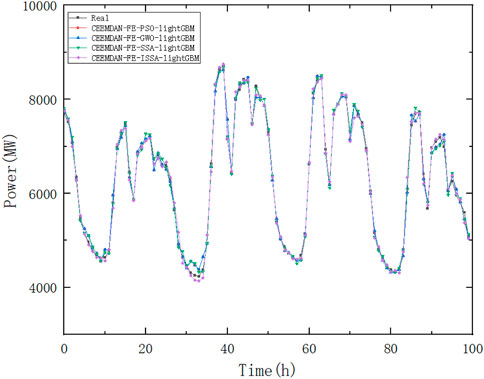
FIGURE 11. Case 1 graph of this paper’s model versus the hybrid model.

As seen in Figure 11 and Table 4, LightGBM outperforms the other two algorithms compared to the single model. Both can contribute to the improvement of the accuracy of the prediction results after the decomposition process or the addition of ISSA algorithm optimization. However, the single processing means are not as effective as the CEEMDAN-FE-ISSA-LightGBM model, and the improvement of the prediction accuracy mainly relies on the tuning of ISSA, while the addition of the FE algorithm has no obvious effect on the improvement of the prediction accuracy, and the improvement of MAE and RMSE is only 0.087% and 0.2%, but in terms of the operation time, this paper. However, the average time of 20 operations of the proposed algorithm is 843.2846 s, which is much smaller than the average time of 20 operations of the CEEMDAN-ISSA-LightGBM algorithm without FE, which is 1,273.3726 s, saving time and improving the efficiency of operations.

TABLE 4

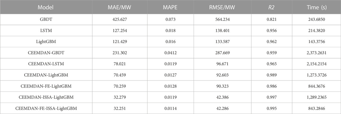
TABLE 4. Error of the proposed model versus a single model in Case 1.

To further verify the effectiveness of the optimization algorithm and compare it with other optimization models, CEEMDAN-FE-PSO-LightGBM, CEEMDAN-FE-GWO-LightGBM, and CEEMDAN-FE-SSA- LightGBM models are developed in this paper.

From Figure 11 and Table 5, the CEEMDAN-FE-ISSA-LightGBM algorithm proposed in this paper has the best results in terms of performance compared with other algorithms. The MAE is 45.59%, 40.74%, and 25.69% lower than the other algorithms; MAPE is 41%, 35.35%, and 13.51% lower than the other algorithms; RMSE is 43.33%, 36.70%, and 17.70% lower than the other algorithms, respectively. It can be seen that the CEEMDAN-FE-ISSA-LightGBM algorithm proposed in this paper has the best prediction effect.

TABLE 5

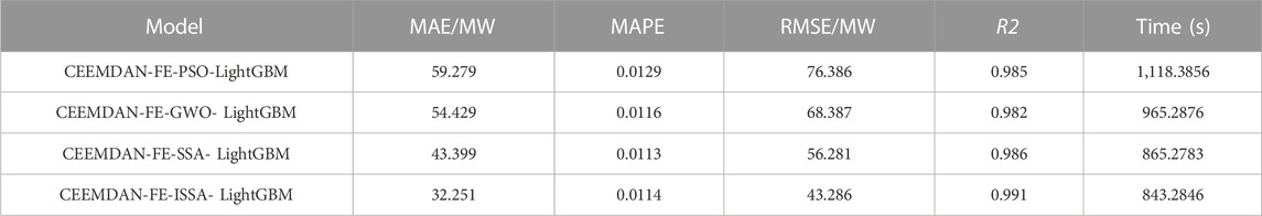
TABLE 5. Error comparison of the proposed model with other hybrid models in Case 1.

5.3.2 Case study 2:1-day time-scale load forecasting

5.3.2.1 Experimental CEEMDAN-FE decomposition of raw load information

From Figure 5, the data for the second set of intra-day average loads is smoother compared to the hourly loads, so its decomposition yields a smaller number of sub-series, as shown in Figure 12.

FIGURE 12

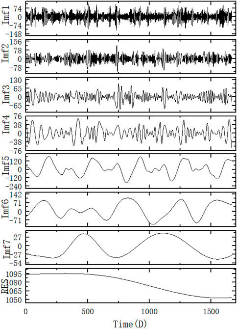
FIGURE 12. Results of the decomposition of Case 2 CEEMDAN.

The fuzzy entropy calculation is performed on the decomposed subsequences one by one to provide a basis for reconstruction, and the results of the fuzzy entropy calculation are shown in Figure 13.

FIGURE 13

FIGURE 13. Fuzzy entropy analysis of the decomposition results of Case 2.

From Figure 13, it can be seen that the fuzzy entropy values of Imf5-Res are similar and can be recombined into a new sequence, and the recombined components are shown in Table 6.

TABLE 6

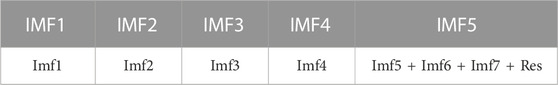
TABLE 6. Recombination of each sequence.

The decomposition results obtained after recombination are shown in Figure 14.

FIGURE 14

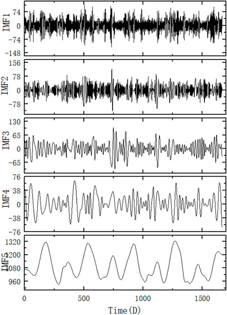
FIGURE 14. CEEMDAN-FE processing results of Case 2.

5.3.2.2 Prediction experiments based on the CEEMDAN-FE-ISSA-LightGBM algorithm

The parameters of the ISSA algorithm in Case 2 are set according to Case 1, and a comparison of the effect with other algorithms is shown in Figure 15.

FIGURE 15

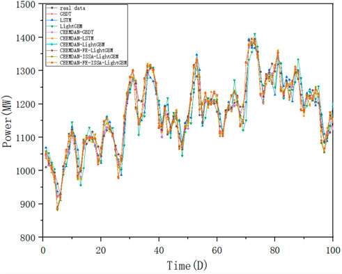
FIGURE 15. Case 2 graph of this paper’s model versus a single model.

As can be seen from Figure 15 and Table 7, the algorithm proposed in this paper is equally effective for short-term electricity load forecasting on a 1-day time scale. The “decomposition-reconstruction-combination” load forecasting model idea, especially the decomposition operation, can effectively reduce the non-smoothness of the original time-series data and improve the accuracy of forecasting. “Reconstruction” can improve the efficiency of prediction by avoiding over-decomposition and reducing the number of operators. The “combination” operation allows the prediction model to work better by optimizing the hyperparameters, further improving prediction efficiency.

TABLE 7

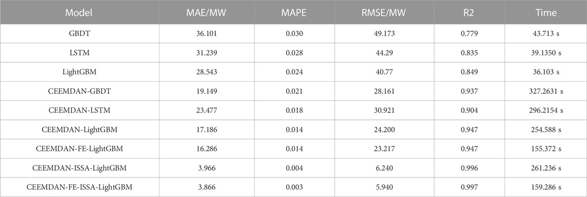
TABLE 7. Error of the proposed model versus a single model in Case 2.

Figure 16 and Table 8 validate the application of the ISSA algorithm proposed in this paper to the model. Compared to other optimization algorithms, it can be seen that ISSA can accomplish hyperparameter optimization of the prediction model more effectively, resulting in better and faster predictions.

FIGURE 16

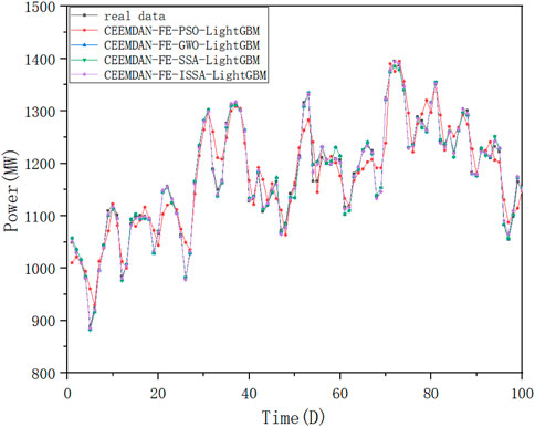
FIGURE 16. Case 2 graph of this paper’s model versus the hybrid model.

TABLE 8

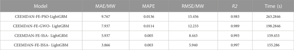
TABLE 8. Error comparison of the proposed model with other hybrid models in Case2.

5.4 Diebold-Mariano (DM) test

DM tests are often used to compare which of two time series forecasting models predicts better results. The DM test allows the validity of the portfolio model to be checked from a statistical point of view.

The null hypothesis indicates that there is no significant difference in the predictions of the two models; the valid hypothesis is that there is a significant difference in the predictive performance of the two models. The null and alternative hypotheses expressing DM detection are as follows.

$\begin{array}{c}{H}_0:E\left[F\left(e_t^1\right)\right]=E\left[F\left(e_t^2\right)\right]\end{array}(33)$

$\begin{array}{c}{H}_1:E\left[F\left(e_t^1\right)\right]=E\left[F\left(e_t^2\right)\right]\end{array}(34)$

where $e_t^1$ and $e_t^2$ are the prediction errors between the predicted and actual values of the proposed model and the other model, and F is the loss function of the prediction errors.

The expression for the DM test is expressed as

$\begin{array}{c}DM=\frac{\frac{{\sum }_{i=1}^n\left(F\left(e_t^1\right)-F\left(e_t^2\right)\right)}{n}}{\sqrt{\frac{S^2}{N}}}{S}^2\end{array}(35)$

where $S^2$ is the estimated variance of $d=F\left(e_t^1\right)-F\left(e_t^2\right)$.

The DM tests for the two time scales are shown in Table 9 and it can be seen from the table that the performance of the proposed combined model in this test is significantly different from all other models. In addition, the minimum DM values for these two time scales are 1.945 and 2.044 respectively. Thus, the proposed combined model significantly outperforms the other models, thus validating the effectiveness of our proposed combined model.

TABLE 9

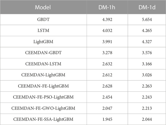
TABLE 9. Error comparison of the proposed model with other hybrid models.

6 Conclusion

The article proposes a prediction method based on the CEEMDAN-FE-ISSA-LightGBM model for the problem of inaccurate prediction caused by strong non-stationarity of electric load. The LightGBM model can accurately grasp its time-series characteristics, and the ISSA algorithm helps the LightGBM algorithm to per-form parameter optimization, so that the data can be better matched with the model structure to achieve efficient prediction and improve the prediction accuracy and efficiency. The results of simulation experiments prove that the error accuracy of the prediction results of the method is improved and the prediction results are better. The case study in this paper demonstrates the following.

1) Compared to single models, combined models are more accurate and efficient in the field of electricity load forecasting.

2) The CEEMDAN-FE algorithm’s “decomposition-reconstruction” process effectively reduces the non-smoothness of the original load data, while avoiding the computational burden of over-decomposition and improving the efficiency of subsequent prediction model construction.

3) The ISSA-LightGBM model allows the hyperparameters to be adjusted individually according to the characteristics of the different sub-sequences so that the overall prediction model can be more closely matched to the sub-sequences and better prediction results can be obtained. The “decomposition-restructuring-combination” process also gives better results for each sub-series, and the linear reorganisation gives better prediction values, with R2 values of 0.97 in both cases.

4) By changing the hyperparameters, the data can be well matched to the model, and the model proposed in this paper has good robustness.

In the future, other factors affecting load output, including temperature and humidity, should be considered to determine if they can further improve prediction accuracy. Meanwhile, this paper mainly uses ISSA-LightGBM to achieve predictions for each sub-series, and the ISSA-LightGBM may not be as effective as it could be with different frequencies per sub-series, and it may be more desirable to subsequently employ multiple predictions to engage in the problem of predicting different sub-series. In addition, the model proposed in this paper can be extended to other time scales and energy fields.

Data availability statement

The original contributions presented in the study are included in the article/supplementary material, further inquiries can be directed to the corresponding author.

Author contributions

ZL basically completed all the contents of this article. ZC reviewed the feasibility and details of the article.

Conflict of interest

Author ZC is employed by Shanghai Architectural Design and Research Institute Co., Ltd.

The remaining author declares that the research was conducted in the absence of any commercial or financial relationships that could be construed as a potential conflict of interest.

Publisher’s note

All claims expressed in this article are solely those of the authors and do not necessarily represent those of their affiliated organizations, or those of the publisher, the editors and the reviewers. Any product that may be evaluated in this article, or claim that may be made by its manufacturer, is not guaranteed or endorsed by the publisher.

References

Baniamerian, A., Asadi, M., and Yavari, E. (2009). “Recurrent wavelet network with new initialization and its application on short-term load forecasting,” in 2009 Third UK Sim European Symposium on Computer Modeling and Simulation, Athens, Greece, November 25–27, 2009, 379–383.

CrossRef Full Text | Google Scholar

Blake, R., Michalkova, L., and Bilan, Y. (2021). Robotic wireless sensor networks, industrial artificial intelligence, and deep learning-assisted smart process planning in sustainable cyber-physical manufacturing systems. J. Self-Governance Manage. Econ. 9, 48–61.

Google Scholar

Chen, T., Huang, W., Wu, R., and Ouyang, H. (2021). Short term load forecasting based on SBiGRU and CEEMDAN-SBiGRU combined model. IEEE Access 9, 89311–89324. doi:10.1109/access.2020.3043043

CrossRef Full Text | Google Scholar

Chen, X., Shi, M., Sun, H., Li, Y., and He, H. (2018). Distributed cooperative control and stability analysis of multiple DC electric springs in a DC microgrid. IEEE Trans. Ind. Electron 65, 5611–5622. doi:10.1109/tie.2017.2779414

CrossRef Full Text | Google Scholar

Choi, S., and Hur, J. (2020). An ensemble learner-based bagging model using past output data for photovoltaic forecasting. Energies 13, 1438. doi:10.3390/en13061438

CrossRef Full Text | Google Scholar

Fan, C., Xiao, L., Ai, Z., Ding, C., and Zheng, J. (2020). Empirical mode decomposition based multi-objective deep belief network for short-term power load forecasting. Neurocomputing 388, 110–123. doi:10.1016/j.neucom.2020.01.031

CrossRef Full Text | Google Scholar

Ge, L., Li, Y., Yan, J., Wang, Y., and Zhang, N. (2021). Short-term load prediction of integrated energy system with wavelet neural network model based on improved particle swarm optimization and chaos optimization algorithm. J. Mod. Power Syst. Clean Energy 9, 1490–1499. doi:10.35833/mpce.2020.000647

CrossRef Full Text | Google Scholar

Goh, H. H., He, B., Liu, H., Zhang, D., Dai, W., Kurniawan, T. A., et al. (2021). Multi-convolution feature extraction and recurrent neural network dependent model for short-term load forecasting. IEEE Access 9, 118528–118540. doi:10.1109/access.2021.3107954

CrossRef Full Text | Google Scholar

Gong, P. Y., Luo, Y. F., Fang, Z. M., and Dou, F. (2021). Short-term power load forecasting method based on attention-BiLSTM-LSTM neural network. J. Comput. Appl. 41, 81–86.

Google Scholar

Guo, S., Guo, Z., and Li, Y. (2022). “Load forecasting model of power grid based on EWM and GRA-ELM,” in 2022 Power System and Green Energy Conference (PSGEC), Shanghai, China, August 25–27, 2022, 1180–1184.

CrossRef Full Text | Google Scholar

Hassan, S., Khosravi, A., Jaafar, J., and Khanesar, M. A. (2016). A systematic design of interval type-2 fuzzy logic system using extreme learning machine for electricity load demand forecasting. Int. J. Elect. Power Energy Syst. 82, 1–10. doi:10.1016/j.ijepes.2016.03.001

CrossRef Full Text | Google Scholar

Kim, J., Cho, S., Ko, K., and Rao, R. R. (2018). “Short-term electric load prediction using multiple linear regression method,” in 2018 IEEE International Conference on Communications, Control, and Computing Technologies for Smart Grids (Smart Grid Comm), Aalborg, Denmark, October 29–November 01, 2018, 1–6.

CrossRef Full Text | Google Scholar

Liu, Q., Shen, Y., Wu, L., Li, J., Zhuang, L., and Wang, S. (2018). A hybrid FCW-EMD and KF-BA-SVM based model for short-term load forecasting. CSEE J. Power Energy Syst. 4, 226–237. doi:10.17775/cseejpes.2016.00080

CrossRef Full Text | Google Scholar

Lv, L., Wu, Z., Zhang, J., Zhang, L., Tan, Z., and Tian, Z. (2022). A VMD and LSTM based hybrid model of load forecasting for power grid security. IEEE Trans. Industrial Inf. 18, 6474–6482. doi:10.1109/tii.2021.3130237

CrossRef Full Text | Google Scholar

Song, J., Jin, L., Xie, Y., and Wei, C. (2021). “Optimized XGBoost based sparrow search algorithm for short-term load forecasting,” in 2021 IEEE International Conference on Computer Science, Artificial Intelligence and Electronic Engineering (CSAIEE), August 20–22, 2021, 213–217.

CrossRef Full Text | Google Scholar

Torres, M. E. (2011). “A complete ensemble empirical mode decomposition with adaptive noise,” in 2011 IEEE International Conference on Acoustics, Speech and Signal Processing (ICASSP), Prague, Czech, May 22-27, 2011, 4144–4147.

CrossRef Full Text | Google Scholar

Wei, L., and Zhen-gang, Z. (2009). “Based on time sequence of ARIMA model in the application of short-term electricity load forecasting,” in 2009 International Conference on Research Challenges in Computer Science, Shanghai, China, December 28-29, 2009, 11–14.

CrossRef Full Text | Google Scholar

Wu, Z., and Wang, B. (2021). An ensemble neural network based on variational mode decomposition and an improved sparrow search algorithm for wind and solar power forecasting. IEEE Access 9, 166709–166719. doi:10.1109/access.2021.3136387

CrossRef Full Text | Google Scholar

Yao, X., Fu, X., and Zong, C. (2022). Short-term load forecasting method based on feature preference strategy and LightGBM-XGboost. IEEE Access 10, 75257–75268. doi:10.1109/access.2022.3192011

CrossRef Full Text | Google Scholar

Zheng, H., Yuan, J., and Chen, L. (2017). Short-term load forecasting using EMD-LSTM neural networks with a xgboost algorithm for feature importance evaluation. Energies 10, 1168. doi:10.3390/en10081168

CrossRef Full Text | Google Scholar