Fault detection in a distribution network using a combination of a discrete wavelet transform and a neural Network’s radial basis function algorithm to detect high-impedance faults

High Impedance Fault detection in a solar photovoltaic (PV) and wind generator integrated power system is described in this paper using discrete wavelet transform and a neural network with radial basis function (NNRBF). For this paper, the integration of solar photovoltaic and wind systems was modelled in a MATLAB/Simulink environment to create an IEEE 13-bus system. Microgrids (MG’s) are mostly powered by renewable energy. Uncertainty about renewables has shifted attention to ensuring a steady supply and long-term viability. It has been addressed in the paper whether or not a small-scale distant end source connection may be made at the terminal of a radial distribution feeder. Some typical power system problems compromise the reliability of the grid’s power supply. To solve this problem, this study suggests a criterion algorithm based on the neural network with radial basis function (NNRBF), and a defect detection method based on the discrete wavelet transform (DWT). The MATLAB/Simulink model of the system is then used to produce fault and travelling wave signals. The db4 wavelet is used to deconstruct the travelling wave signals into detail and approximate signals, which are then combined with the data from the two-terminal travelling wave localization approach for fault detection. After that, the optimal maximum coefficients of the wavelets are extracted and fed into the proposed radial basis function neural network (NNRBF). The results show that both the criterion algorithm and the fault detection algorithm are reliable in their assessments of whether or not faults exist in the power system, and that neither algorithm is particularly sensitive to variations in fault type, fault detection, fault initial angle, or transition resistance. After that, the optimal maximum coefficients of the wavelets are extracted and fed into the proposed radial basis function neural network (NNRBF). Overhead distribution system faults are simulated in Matlab/Simulink, and the technique is rigorously validated across a wide range of system situations. It has been shown through simulations that the proposed method can be relied upon to successfully and dependably protect high impedance fault (Hi-Z).

1 Introduction

The widespread recognition of the negative effects of fossil fuel consumption on the environment is a primary cause of this issue. Use of sustainable materials. Hydroelectric power, PV power, wind power, and micro-turbines are all examples of renewable energy sources that can help meet the growing demand for electricity without increasing pollution. Although wind and PV energy show the most promise, their utilization is limited by the fact that they are unpredictable and intermittent, which results in unreliable economic dispatch (Kroposki et al., 2017; Qazi et al., 2019). MG’s in remote places that run on renewable energy sources like wind and solar PV are becoming more reliable thanks to the installation of energy storage (Billinton and Karki, 2001; Kroposki et al., 2017). The complementary nature of solar photovoltaics and wind power is an inherent benefit (Al-Masri and Ehsani, 2015). Maximum power point (MPP) extraction is used to get the most efficient amount of energy from the wind and sun. Maximum power point for solar is found using the incremental conductance (De Brito et al., 2012) scheme, whereas for wind it is found using the estimation based perturb and observe (EP&O) (Xiao et al., 2011) scheme. Traditional P&O, MPP schemes perform poorly under conditions of rapid change in the surrounding environment, which can cause tracking to lag or even fail (Ahmed and Salam, 2018). Since the control parameter is an incremental step, it struggles to deliver sufficient dynamic performance. Finding the sweet spot for parameter size can be tricky. The inverter output fluctuates because of the dominating oscillation close to the MPP. EPO offers a more in-depth evaluation of the MPP than what is available through the standard P&O technique. Due to the extremely non-linear nature of the wind, the MPP can only be attained by a combination of the perturb procedure’s exhaustive search of the search zone and the estimate procedure’s compensation for the perturb procedure’s inefficiencies as the wind speed varies. Therefore, PV and wind power together can help with the issue of long-term intermittency. This makes it all the more important to design a solid protection architecture capable of detecting and categorising system failures in order to ensure MG’s safe and reliable functioning. Numerous studies were conducted to identify faults, categorize them, and isolate them to lessen the frequency and duration of outages in the transmission and distribution networks. HIF is an annoying system anomaly. A HIF is formed whenever an electrical conductor comes into contact with a high-resistance item, such as a branch, sand, or asphalt. In a grounded system, its fault current is typically between 0 and 75 A, displaying asymmetrical, intermittent, and non-linear arcing behavior (Costa et al., 2015; Wang et al., 2016). Due to the lower current magnitude, the over current relay often fails to detect the HIF in the system, leading to a cascading failure of the system and putting people and their belongings in danger (Sedighi et al., 2005a). Furthermore, the spread of HIF to otherwise functional areas of the grid might cause a domino effect of failure throughout the entire system (Kavi et al., 2018; Santos et al., 2017). To investigate the impact of HIF on distribution networks, a mathematical model is proposed in (Yu et al., 2008) in the form of a non-linear partial differential equation.

According to Figure 1, the most common causes of failures in an urban distribution system are external variables, natural factors, and improper maintenance and operation. The presence of a path to ground is not required for a Hi-Z fault to occur, and the presence of such a path has no bearing on the detection of a Hi-Z fault. Current paper, however, employs a DWT and NNRBF for a distribution network to detect HIF in wind and solar PV power networks. Overhead power lines are the typical method of delivering electricity to homes and businesses. Due to exposure to varying climatic conditions, these are more likely to have power outages. It may be possible to readily detect and localize a subset of these malfunctions. However, there are not many malfunctions that cannot be spotted by standard safety measures (AsghariGovar et al., 2018). Equipment attached to the supply line can be harmed if the distribution system is allowed to run for hours or days with unidentified HIF. Furthermore, the analysis reveals that electric arcs emit a random, unpredictable, and unbalanced current that is then followed by HIF (Chen et al., 2016). Because distribution infrastructure is often located near densely inhabited regions, deaths from electrical arcs are all too often. Despite the fact that the detection of HIFs has been a topic of study since the early 1970s, more work remains to be done to shed light on the process. Using the ratio of harmonics at lower orders, as described in (Emanuel et al., 1990). One problem of this type of method is that it requires setting a number of threshold values, which might negatively impact the detection method’s efficiency. Methods based on time-frequency analysis have shown promising results in the identification procedure (Samantaray et al., 2008; Ghaderi et al., 2014). However, the rate of erroneous detection is demonstrated to be a significant barrier to real-world implementations. Faults can be identified by comparing the current or voltage signal before and after the fault occurred, using techniques that operate in the time domain. There are minimal problems associated with an unbalanced network when using the mathematical morphology-based time domain methods presented in (Gautam and Brahma, 2012; Sekar and Mohanty, 2017). Since the DWT can identify both the frequency component and its temporal position, it has found widespread application in signal processing. There has been more than a decade of experience protecting electrical grids with these techniques. Although DWT based techniques are providing a good detection rate with linear loads (Sarlak and Shahrtash, 2011), there is no evidence of non-linear loads inclusion with the systems while detecting HIFs except in (Chen et al., 2016). All the way through the power distribution networks, the number of non-linear loads (NLLs) has been steadily rising in recent years. While NLLs are a key part of the puzzle when it comes to modelling and building viable HIF detection algorithms, a large proportion of currently available methods ignore them. Similarities between NLL and HIF features will reduce the efficacy of current approaches. The majority of current proposals for defect diagnosis can be broken down into two groups: frequency domain feature identification methods and adaptive detection techniques. Three of the most common methods for finding features in the frequency domain are the Fourier transform, the wavelet transform, and the Hilbert-Huang transform. These days, adaptive detection strategies typically use either expert systems or neural networks. These theoretical studies have produced useful insights, but they are not without their faults. While the single-ended travelling wave fault location approach is commonly used, detecting the wave head is difficult, and placement accuracy is low (Santos et al., 2016). Empirical mode decomposition (EMD) was optimized using integrated EMD (see (Mahari and Seyedi, 2015)). While this approach did not suffer from modal aliasing, it did introduce fake components, which led to poor placement precision. An approach to fault phase selection is proposed in (Sedighi et al., 2005b) that makes use of the high-order multi-resolution singular entropy of active fault components. Though this method works regardless of fault type, fault detection, or transition resistance, finding the right cutoff value can be challenging. When compared to the Fourier transform, the wavelet transform is a marked improvement. Since the Fourier transform is unable to fully express the time-frequency localization property of non-stationary signals, the wavelet transform is used instead. In addition to its strength as a general tool for waveform analysis, the Wavelet Transform excels at analyzing waveforms at the time-frequency level. As a result, it can quickly and accurately identify the signal’s focal point, analyze its degree of distortion, and extract precise information from the time and frequency domains (Bakar et al., 2014; He et al., 2014). Fault detection in the fars power distribution system was given a boost in accuracy and efficiency thanks to wavelet transform’s application in (Soualhi et al., 2015). When conducting signal analysis using a wavelet transform, extracting both approximation and detailed features is a crucial step. Find the best decomposition level, partition features as finely as feasible, and keep errors isolated from features. Both feature component extraction and fault detection accuracy suffer from the current approaches’ reliance on either manually set threshold control or testing with retrieved trend via wavelet transform. With the neural network serving as a model for the neuron network in the human brain, the values of the input layer neurons are mapped to the values of the output layer neurons, establishing an implicit function relationship between the input and the output. An asymmetrical fault line searching and locating scheme is developed using the fault direction distinguishing method and its associated communication system. A more up-to-date method for locating faults in a distribution network that includes DG units is the multi-layer perceptron neural network (MLPNN) (Jiang et al., 2003; Gafoor et al., 2014). As a result of the MLPNN’s structure and training algorithm, however, its speed is not ideal for applications requiring rapid and precise fault finding (Kordestani et al., 2016; Bayrak, 2018). Non-linear, prior-data-driven processing is employed by the network. Compared to traditional methods of diagnosis, it gives room for more imaginative data manipulation. In contrast, the neural network can learn quickly and tolerates errors better during diagnosis. However, it is not without its flaws. When it comes to power system failure diagnosis, gathering enough data to train a neural network is difficult. It was easy for the neural network to get mired in a cycle of local minima. This study suggests a fault detection system based on wavelet transform and the chaotic neural network as a solution to these problems. The chaotic neural network avoids the drawback of getting stuck at the local optimum. It also has excellent error-handling and associative memory features. With the advent of the internet of things and the cloud-edge-collaboration framework, the authors of (Tonelli-Neto et al., 2017) introduce a DWT and NNRBF for detecting HIF by fusing together information from different distribution networks. To identify HIF in an IEEE 13-bus distribution network, the authors (Rezaei and Haghifam, 2008) opted on a fault-based strategy.

FIGURE 1

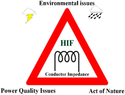
FIGURE 1. Causes of HIF.

The following outlines the primary inspiration and contribution of this work.

• Electrical Distribution to Rural Areas: Using RESs with energy storage makes it economically feasible to bring electricity to rural areas. Solar PV array, wind turbine, and battery all work together to minimize maintenance costs and maximize clean energy production. When the sun, the wind, the batteries, and the load all align, the adopted control will carry out the specified action.

• One MG based on VSI control is created. In addition, a diode rectifier is used to change the AC current produced by PMBLDCG’s wind turbines into DC current. Therefore, the overall system cost has decreased thanks to this topology.

• The PMBLDCG saves money by not requiring expensive sensors for MPPT control (like speed/position/wind speed sensors). As the MPP and power converter control become independent, the large operating range and control dependability of a second stage solar design are worth the additional components.

• Renewable energy source used are maintenance free and having high efficiency.

• A neural network called NNRBF is proposed as the basis for an algorithm to select fault phases. An NNRBF neural network is trained on fault features extracted using wavelets, and its output is correlated with inputs to determine the fault type. When it comes to fault and transition resistance, the algorithm is stable.

• There is a proposal for a wavelet-transform-based fault detection algorithm with two terminals. The db4 wavelet is used to detect the travelling wave head to diagnose the issue. This algorithm’s fault-detection accuracy is excellent, and it is robust against variations in fault type and transition resistance.

2 Solar PV energy: A brief description

Non-linearity in the I-V curve is a feature of PV cells, and it changes as the cells are exposed to more or less sunlight and are heated or cooled. An ideal solar cell is a circuit that includes a diode and a parallel current source. Yet, we model the losses caused by these cells using the series resistance (Rse) and the parallel resistance (Rsh). This is why the PV cell’s orbital model under real-world conditions is shown in Figure 2. RSH has a much higher market value than RS does. Similarly, the Iph source current is zero in total darkness (Zayandehroodi et al., 2010a; Zayandehroodi et al., 2010b).

FIGURE 2

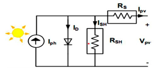
FIGURE 2. PV cell circuit model (Chatrenour et al., 2017).

2.1 The PV module

In a cell, losses are proportional to the resistance in the corresponding circuit. Losses in a cell occur due to multiple processes, including the reflection of incident light at the cell surface, the absorption of photons without electrons and free holes, and the redistribution of electrons and voids. The following equation expresses the solar cell’s distinctive behavior as shown in Figure 2 (Chatrenour et al., 2017).

$I_{pv}=I_{ph}-I_D-I_{SH}(1)$

Where current PV (Ipv), diode current (ID), and diode voltage (Vd). I_SH = V_pv + I_pv, where Ipv is the output current, Vpv is the input voltage, RS and RSH are the solar cell’s corresponding series and parallel resistance, and RS/RSH is the leakage current. Shockley diodes have a voltage-current characteristic, and that characteristic can be written as a formula for the diode current, ID.

$I_D=I_O\left(e^{\frac{v_D}{{aV}_t}}-1\right)(2)$

Here, Io is the reverse saturation current; VD = Vpv + IpvRS is the diode voltage; a is the diode ideal constant;

$V_t=\frac{N_s\cdot k_b}{e}T$ T is the operating temperature of the solar cell; Ns is the number of series cells; kb is the Boltzmann constant; e is the electron charge; and T is the diode’s thermal voltage. Adding Eq. 2 to the first equation yields the solar panel’s defining equation, which is as follows:

$I_{PV}=I_{ph}-I_o\left(e\frac{V_{PV}+I_{PV}{R}_S}{a{V}_t}-1\right)-\frac{V_{PV}+I_{PV}{R}_S}{R_{SH}}(3)$

The value of the photovoltaic current Ipv is related to the variations in light intensity and temperature as shown in Eq. 3.

2.2 DC to DC boost converter configuration

In order to maintain a constant load voltage between the PV array and inverter, a DC-DC boost converter is employed (Necaibia et al., 2017). As the voltage produced by PV systems is typically insufficient to power loads directly, this is an essential component of PV applications. In this study, a novel ANN control based MPPT approach was implemented to maximize power output from a DC-DC boost converter before feeding it into the input of an RS MLI. By calculating the duty cycle for the converter switch and running at a high switching frequency, Maximum Power Point Tracking (MPPT) is a technique for getting the most power out of PV panels. If the converter is in continuous conduction mode, the current through the inductor is always present (Abdullah et al., 2012). We provide duty cycle, inductor (L), and capacitor (C) formulas below.

$\frac{V_{out}}{V_{in}}=\frac{1}{1-D}(4)$

$inductor\left(L\right)=\frac{V_{in}\times D\times T}{{\Delta }_{iL}}(5)$

$Capacitor\left(C\right)=\frac{V_{out}\times D}{R\times \Delta V_{out}\times f}(6)$

Vin and V0 are the boost converter’s input and output voltages; D is the duty cycle. D > 1 means output voltage > input voltage. Figure 3 depicts a DC-DC boost converter with PV integration and the ANN control based MPPT approach for maximizing PV duty cycle.

FIGURE 3

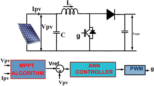
FIGURE 3. PV system configuration using MPPT and DC–DC boost converter (Yahya and Yahya, 2023).

When a boost converter is used in conjunction with a PV array, it is discovered that the average current from the PV array increases as the duty cycle rises, resulting in a decrease in the voltage from the PV array as a whole. In order to raise the PV array’s break-even point, D modifies its V-I characteristic. When D is decreased, the average current from a PV array drops while the voltage is raised. If the PV array’s operating point moves to the right, it means the array’s output has been modified. In order to keep the DC voltage output at the VSC terminal constant, the DC-DC converter’s value of D is automatically adjusted using the perturb and absorb MPPT approach.

In (Yahya and Yahya, 2023), DC-DC boost converter technology to track the maximum power of a photovoltaic (PV) system using a maximum power point tracking (MPPT) controller based on a modified version of particle swarm optimization (MPSO). A DC-DC boost converter was utilized to increase the input DC voltage of the PV module. The boost converter supplied power for the DC-AC multilevel PWM inverter, which supplied the output AC voltage to a single inductive load. It is common practise to employ cascaded multilayer inverters to condition power in renewable energy applications due to its simplicity and low cost. Modulations in the DC link capacitor voltage result in low order harmonics and inter harmonics at the output of the multilevel inverter. The lowest number of harmonics is achieved using phase disposition pulse width modulation (PDPWM). Energy from the inverter cells.

2.3 Description of wind source

Solar and wind power dominate the renewable energy market due to their low environmental impact and high irradiation and kinetic energy output, respectively. Figure 4 depicted wind energy conversion system (WECS), purpose of WECS is to exploit the kinetic energy of wind for use in mechanical power generation. Low efficiency, non-linearity and unpredictability in wind speed, and high construction cost are all factors that prevent widespread adoption of wind energy (Manwell et al., 2010). Therefore, a control algorithm is necessary to optimize performance and cut expenses. Using a wind turbine, one can convert wind energy into electricity DWT. DWT are made up of blades and a motorized device. An AC-DC and DC-DC converter are required on the control side. In this study, a horizontal wind turbine with variable speed was used. Since variable speed turbines can generate electricity at varying wind speeds, they have a higher efficiency rating than fixed speed turbines (Nurzaman et al., 2017). In this study, a permanent-magnet synchronous generator is used (PMSG). PMSG’s high efficiency at low speeds has made it a popular choice for use in small-scale wind turbines. On the control side, an ANN control based MPPT algorithm locates and maintains the turbine’s maximum power point, maximizing its efficiency. Here, we present a DC-DC boost converter that is managed by a ANN control based MPPT algorithm and integrated into a wind power generation setup. In this paper, we’ll go over the results of a simulation test of ANN control based MPPT controllers for a residential wind turbine run through the Simulink MATLAB modelling environment.

FIGURE 4

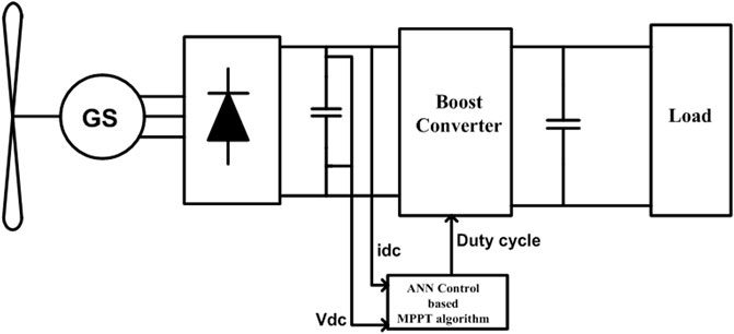
FIGURE 4. WECS configuration (Vas, 1999).

Wind turbines’ peak mechanical power, stated as (Abdullah et al., 2011)

$P_{\mathit{max}}=\frac{1}{2}\rho C_{p}A{V}_w^3(7)$

Where ρ is the density of the air (in kg/m3), A is the swept area of the rotor blades (in m2), and Vw is the speed of the wind (in metres per second). Cp is the power coefficient, is written as (Gite and Pawar, 2017).

$c_p=c_1\left(\frac{C_2}{{\lambda }_i}-C_3\beta -C_4\right){e_5}^{\frac{-C}{{\lambda }_i}}+C_6\lambda (8)$

$\frac{1}{{\lambda }_i}=\frac{1}{\lambda +0.08\beta }-\frac{0.035}{{\beta }^3+1}(9)$

$\lambda ={\omega }_m*\frac{R}{V_w}(10)$

C1 to C6 are rotor-specific. In this paper, C1 = 20, C2 = 140, C3 = 0.4, C4 = 28, C5 = 21, and C6 = 0.068.

2.4 Combined boost converter, rectifier, and PMSG in series

Figure 5 is an electrical circuit schematic that depicts the PMSG, rectifier, and boost converter all in one convenient location. This model’s goal is to find the relationship between DC grid load current and turbine.

FIGURE 5

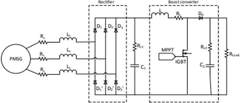
FIGURE 5. Electrical circuit schematic that depicts the PMSG, rectifier, and boost converter (Mishra and Panigrahi, 2019).

The current in dq reference frame represented as

$\frac{d}{dt}\left[\begin{array}{c}{i}_{sd}\\ i_{sq}\end{array}\right]=-\left[\begin{array}{cc}\frac{R_s}{L_{sd}}& -\frac{L_{sd}}{L_{sq}}{\omega }_e\\ \frac{L_{sd}}{L_{sq}}{\omega }_e& \frac{R_s}{L_{sq}}\end{array}\right]\left[\begin{array}{c}{i}_{sd}\\ i_{sq}\end{array}\right]+\left[\begin{array}{cc}\frac{1}{L_{sd}}& 0\\ 0& \frac{1}{L_{sq}}\end{array}\right]\left[\begin{array}{c}{v}_{sd}\\ v_{sq}\end{array}\right]$( 11)

Thus, the expression for the mechanical equivalent torque of an electromagnetic force and the mechanical torque of a machine can be written as

$Te=N\left\{{\mathrm{\Psi }}_f+\left(L_{sd}-L_{sq}\right)i_{sd}\right\}{i}_{sq}(12)$

$Tm=\frac{P}{{\omega }_m}=\frac{1}{2}\rho \pi R^2{C}_P\frac{V_w^3}{{\omega }_m}(13)$

Hence the rotor speed can be calculated

$\frac{d_{\omega }}{d_t}=\frac{Te-Tm-B{\omega }_m}{j_t+j_p}(14)$

2.5 MPPT

A MPPT algorithm known as P&O is utilized to improve performance is shown in Figure 6. The turbine will be operating at its maximum possible efficiency with the help of MPPT. P&O algorithms function by modifying a control parameter and observing the resulting change in output (Kavaskar and Mohanty, 2019). This algorithm is simple, effective, and does not call for any additional hardware or sensors.

$\Delta P=P\left(k\right)-P\left(k-1\right)(15)$

FIGURE 6

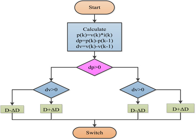
FIGURE 6. MPPT P&O flowchart.

Delta D rises when P is positive and Vs. is negative. If P and the voltage change are positive, delta D will fall. Delta D decreases for a positive voltage change and negative P. If both P and the voltage change are negative, then delta D is too (Alsafasfeh et al., 2012).

3 Systematic illustration of the IEEE-13 bus

The proposed NNRBF classification performance was measured using an IEEE 13-bus network model with high impedance fault, symmetrical and unsymmetrical faults, switching events (heavy load and capacitor bank), and transformer current. The MATLAB/Simulink software environment was used to design the system, which includes a 300 kW solar PV unit (operating under STC) and several load facilities. In this study, an IEEE 13-bus network model was used to evaluate DWT and NNRBF classifiers under high-impedance, symmetrical, and asymmetrical failure conditions. MATLAB/Simulink was used to generate the IEEE 13 bus network model in Figure 7. The test system is connected to the grid with a 200 kVA, 4.16 kV/25 kV transformer (100 MVA, 25 kV, 50 Hz). For the purpose of validating the proposed RNN based classifier’s ability to recognize HIF, it was subjected to a battery of tests across a wide range of operating conditions, including normal operation, switching events (capacitor bank and heavy load), transformer inrush current, and abnormal operation (symmetrical and unsymmetrical faults: single line ground, double line, double line to ground, and three-phase fault). The 300 kWp of solar PV comes from three 100 kW PV modules. Each solar cell in the PV array and its specific configuration are described. (Samet et al., 2017). Provides details on modelling transmission line parameters and load. Both normal and unusual circumstances were used to test the classifier’s capacity to identify HIF (symmetrical and unsymmetrical faults: single line ground, double line, double line to ground and three-phase fault).

FIGURE 7

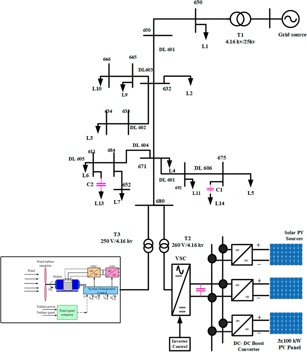
FIGURE 7. IEEE-13 Bus system with the solar PV system & WECS (Mishra and Yadav, 2019).

3.1 The characteristics curve of the PV module

Both the input voltage and output current of the PV array play a role in the I-V and P-V curves that define the PV module. Insulation-voltage and potential-voltage plots. This graphic depicts as MPP at a given temperature and radiation level (where 25°C is assumed for the temperature and 100 W/m2 is assumed for the radiation level). This is the sweet spot for maximizing both power output and efficiency from a PV module. In this case, the MPP is the general maximum, which is another name for the MPP.

Solar cell current (a) and power output (voltage) (b) are shown as a function of solar irradiance (W/m2) in Figure 8. The two most important parts of a PV system are the DC-DC boost converter and the DC-AC VSI. As a result of the boost converter, the 280 V DC maximum power point of the PV unit is increased to 480 V (to 500 V). To achieve maximum power tracking, the MPPT controller’s incremental conductance approach was used to vary the DC-DC boost converter’s duty cycle in response to changes in solar irradiance. We analyzed a three-level IGBT bridge circuit for a PV inverter (VSI) using pulse width modulation (switching frequency of 1980 Hz). The inverter uses synchronous reference frame theory and two-control to regulate the AC voltage at the output. The inverter’s 260 V AC output is increased to 4.16 kV so that it can be connected to the IEEE-13 bus power system network.

FIGURE 8

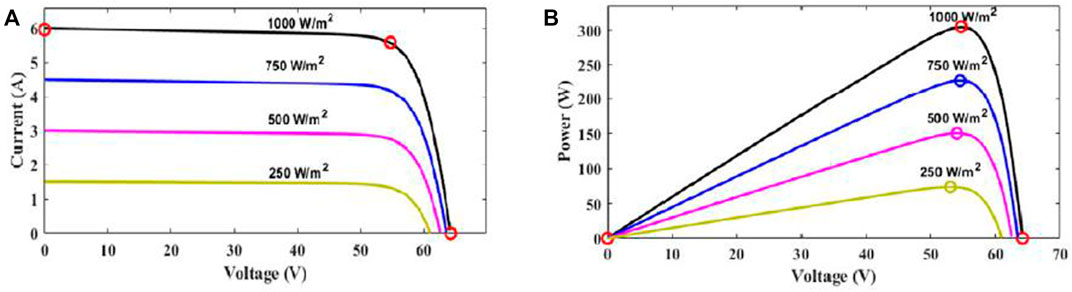
FIGURE 8. (A) Characteristics of the current-voltage curve of a PV array, (B) power-voltage characteristics of PV array.

4 High impedance fault model

Based on the Emanuel model (Gomes et al., 2018), (James et al., 2017) and illustrated in Figure 9, an anti-parallel diode model is used to simulate the waveform features of the HIF current. The ideal HIF V-I characteristics are achieved by adjusting the HIF model parameters V_p, V_n, R_p, and Rn from 550 to 7500 V, 1,100–9000 V, 110 to 4,000, and 120 to 4,000, respectively. HIF’s current and voltage waveforms when sampling at 600V, 1100V, and 120R are depicted in Figure 9A and Figure 9B, respectively. Current waveform is found to be non-linear, asymmetrical, and contain harmonics when HIF model is taken into account. In addition, FFT examination revealed that there was a 3.94% and 11.7% content of second- and third-order harmonics, respectively.

FIGURE 9

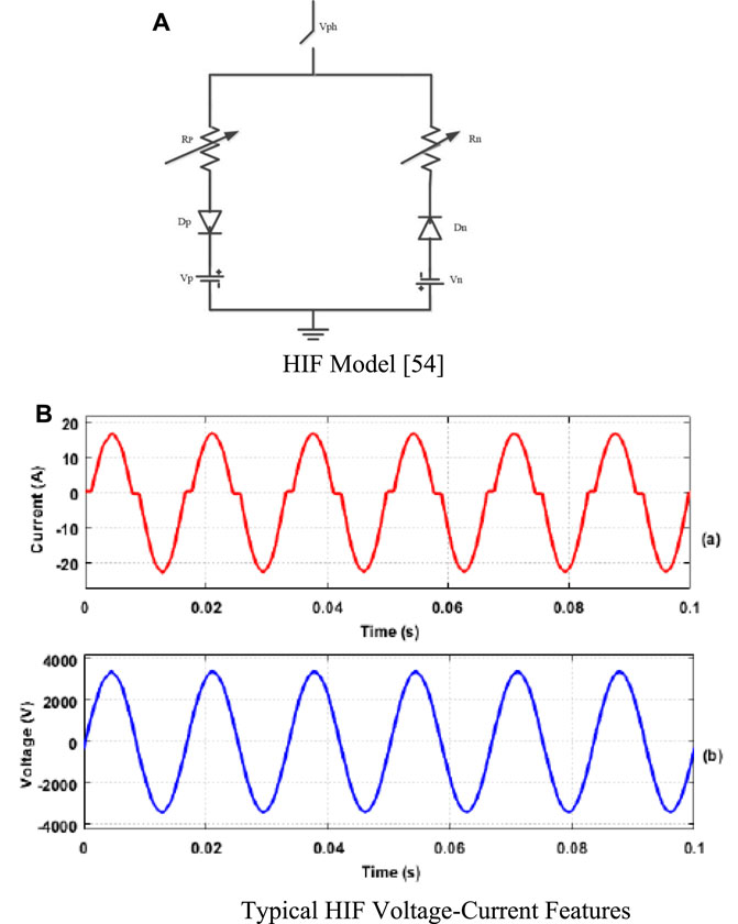
FIGURE 9. (A) HIF model (James et al., 2017) (B) Typical HIF voltage-current features.

4.1 Methodology proposed for the detection of HIF

Using a Figure 10 diagram of the MV distribution power system’s solar PV and wind integrated power network, this part discusses the identification of HIF using intelligent classifiers following the below 4steps.

• Create disturbances in MATLAB/Simulink to obtain faulty existing data.

• To train the classifiers, we have taken samples of the current indicative of a fault using the mother wavelet daubechies4 and then use those samples’ standard deviation (SD) values as the features.

• Data gathered from the discrete wavelet transform (DDWT) during various power system disturbances was used to train artificial intelligence-based classifiers.

• To ensure the classifiers can distinguish the HIF from other power system disturbances including three-phase faults, line-to-ground faults, line-to-line faults, and double line-to-ground faults, they are put through their paces with a variety of test cases. In order to ensure the system’s continued security and dependability, this procedure is repeated during each cycle of operation. Furthermore, as the protective relay is insensitive to fluctuations, the system continued to function normally when the irradiance of the solar and the speed of the wind both fluctuated without triggering any abnormalities.

FIGURE 10

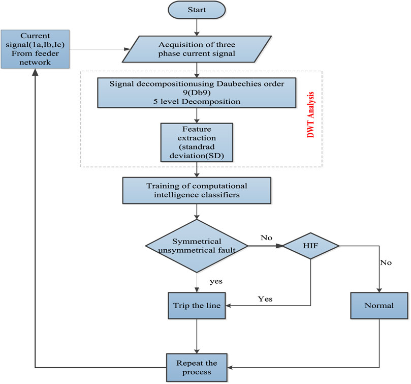
FIGURE 10. Schematic representation of the fault tolerant classification.

4.2 The DWT analysis for data collection

The DWT is a powerful method for separating a transient signal into its constituent parts, which it then displays in the domain of time-frequency instead of the conventional time domain (Elkalashy et al., 2008). The basic concept is to analyze the signal by expanding and contracting it. A continuous signal f (t) is defined in both CDWT and DWT, with the definition provided by Eq. 16.

$CWT\left(a,b\right)=\left[\frac{1}{\sqrt{a}}\underset{-\infty }{\overset{\infty }{{\displaystyle \int }}}f\left(t\right)*h\left(t-\frac{b}{a}\right)d_t\right](16)$

The mother wavelet is the initial point from which a wavelet feature is formed. CDWT is an alternate method for avoiding the same resolution issue that plagues STFT. In contrast to the DWT technique, however, this one has low redundancy during signal reconstruction. The DWT is an effective data technique for signal analysis because it permits the signal to be sampled with distinct peaks. For decades, this sophisticated and powerful instrument has been employed to regulate the safety switches. There are other ways to compute time and frequency information, such as with a fast Fourier transform (FFT), a short-time Fourier transform (STFT), or a continuous- (CDWT), but DWT has been utilized because of its quick computing speed and precision (Chen et al., 2016). Since this is the case, we can express DWT as Eq. 17.

$DWT\left(m,k\right)=\left[\frac{1}{\sqrt{a_0^m}}{\displaystyle \sum }_{n}f\left(n\right)*h\left(\frac{k-n{a}_0^m}{a_0^m}\right)\right](17)$

Algorithm

Below (Chen et al., 2016) we display the various decomposition levels of the signal X(n). Here are the procedures for signal decomposition:

First, through a denoising process, the original X(n) is decomposed into a series of levels.

Choosing a subset of levels from which to reconstruct the signal is the second stage.

Third, re-create the signal using the values you’ve chosen.

In Step 4, you’ll choose the sampling rate, window size, decomposition levels, and mother wavelet.

Where n and m are integers, h is the wavelet function, $a_0^m$ and $n{a}_0^m$ are sizing and interpretation constants, respectively. By using DWT, one can separate a signal into its low-frequency g(n) and high-frequency h(n) approximation and detailed coefficients, respectively as shown in Figure 11. This process of successive approximation is repeated until the signal has been decomposed into a large number of low-resolution sub-signals. In comparison to the Haar wavelet, the Daubechies 4 (db4) is a more effective frequency extractor, it was chosen as the mother wavelet for fault detection in this work. And unlike Coiflet and Meyer wavelets, it reduces signal redundancy and satisfies Parsevall’s theorem (Daubecheis, 1992). The condition shown in Eq. 18 represents the optimal decomposition of L-levels

$N=2^L(18)$

Where N is the level, and L is the length.

$B=\frac{F}{2^{L+1}}(19)$

FIGURE 11

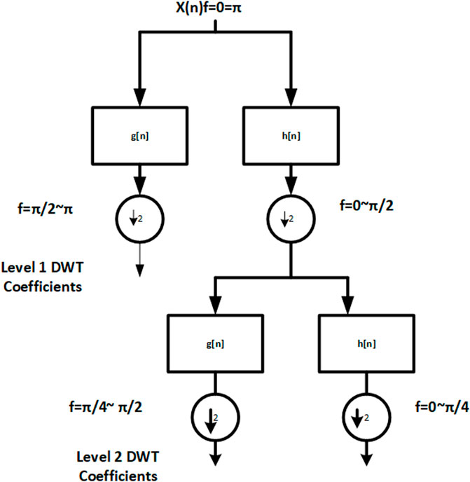
FIGURE 11. DWT decomposition of signal (Daubecheis, 1992).

From Eqs. 19, B is the level-to-level bandwidth in hertz, and F is the sample rate in hertz. In order to divide the signal into its component parts, a sampling rate of 20 kHz is being considered, with each phase of the current signal receiving 800 samples over a length of 5,000 points. Using Eq. 18, we can determine the different band frequencies that were captured at each level, and they are as follows: Approximation is made using the detailed coefficient d4, which represents frequencies from 5 to 2.5 kHz, 2.5 to 1.25 kHz, 1.25 to 0.625 kHz, and 0.625 to 0.3125 kHz, respectively. In the proposed study, the mother wavelet of db4 is used with detailed coefficients on 5 levels for varied fault current signals captured throughout each cycle.

4.3 The effectiveness of NNRBF for fault detection in a DG-enabled distribution network

NNRBFs are trained with data sets generated from short circuit simulations at all line sections accounting for four different types of failures, and then applied to the problem of fault detection in a simulated DG-based distribution system. By analyzing the three-phase currents coming from the main source at the feeding substation, it is possible to identify a single-phase-to-ground fault, a phase-to-phase fault, a two-phase-to-ground fault, or a three-phase fault. In order to standardize the fault currents in the three-phase output at the main source or feeder substation, the maximum fault currents for each fault type are calculated. This equation is used to standardize currents (Yu et al., 2008):

$I_{normal}=\frac{I}{I_{\max }}(20)$

The maximum fault current, or Imax, is the product of the fault current and the fault type, and it varies depending on the nature of the defect. The normalized three-phase fault currents are used to classify various fault types. With k input neurons and m hidden neurons, the NNRBF is a three-layer feed-forward neural network. The input layer feeds data into the hidden layer, while the hidden layer is made up of neurons with radial basis activation functions. In Figure 12 we see a typical NNRBF, and in Figure 12 we see an NNRBF used for training.

FIGURE 12

FIGURE 12. A generic architecture of the NNRBF.

There are several calculations taken into account during NNRBF training. Input k-dimensional vector X is used to calculate a scalar value by the network, which is then output.

$Y=f\left(X\right)=w_0+{\displaystyle \sum }_{i=1}^m{w}_i\varphi \left(D_i\right)(21)$

Where (Di) is the RBF and (w0) is the bias, (wi) is the weight parameter, (m) is the number of hidden-layer nodes, and (m) is the bias.

The Gaussian function is used as the RBF in this investigation, and it is given by.

$\varnothing \left(D_i\right)\exp \left(\frac{-D_i^2}{{\sigma }^2}\right)(22)$

$D_i=\sqrt{{\displaystyle \sum }_{j=1}^k{\left(X_j-C_{ji}\right)}^2}(23)$

Di is the distance between the input vector X and each data centre, where is the radius of the cluster represented by the centre node. Di, the distance between two points, is typically calculated using the Euclidean norm and is presented as a cypher layer in (Yu et al., 2008). Figure 13 depicts the training procedures for the RBFNN and how they are implemented.

FIGURE 13

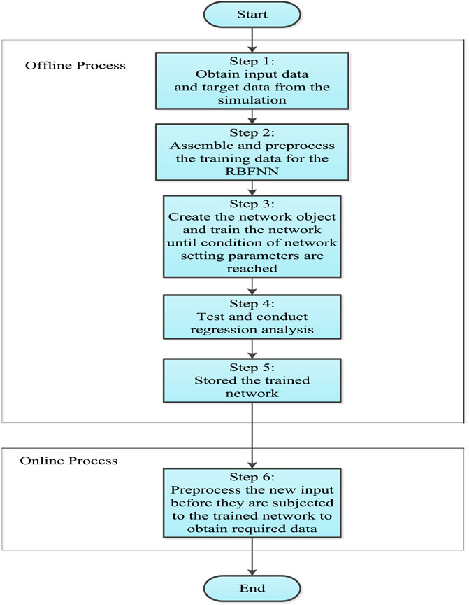
FIGURE 13. Implementation procedures in the training of the NNRBF.

The RBFNNs were implemented in the MATLAB software for the fault detection technique, and training data was generated in the Dig SILENT Power Factory 14.0.523 software by simulating various faults created at the 5th BUS of each line. We can extract the fault distance from each source and the number of defective lines from the RBFNNs’ target vector by running simulations. Here, we break down the inputs and outputs of the training data that was used to hone the generated RBFNNs.

4.3.1 A. First RBFNN

Nine neurons are used as input, and these are the short circuit currents in each source’s three phases (5th BUS). Three neurons are used as output, and these are the fault detection in the main source and two DG units (DS).

4.3.2 Second RBFNN

In this case, there are three input neurons representing the distances to the three potential sources of the fault, and one output neuron representing the actual number of faulty wires. There are about 138 training and testing data sets available, with 80% used for training the RBFNNs and the remaining 20% used for testing their efficacy. Mean square error (MSE) is used in neural networks as a measure of performance. The maximum epoch for training any of the RBFNNs is set to 100, and the mean square error is kept below 0.0002. The trained RBFNNs are then put through their paces after fault classification.

5 Results and discussions

Data is gathered for analysis and classifier training/testing after faults are applied to a number of buses across the 13-bus system. When doing this research, we used eighty percent of the data for training our classifiers and twenty percent for testing. Initial network simulations were performed in MATLAB/Simulink, yielding results for steady-state, transient and conventional faults (LG, LL, LLG, and LLLG incidence), as well as HIF. Maximum HIF occurs when the load current exceeds the fault current. During this instance, the HIF model observed a non-linear connection between voltage and current, which is seen in Figure 14.

FIGURE 14

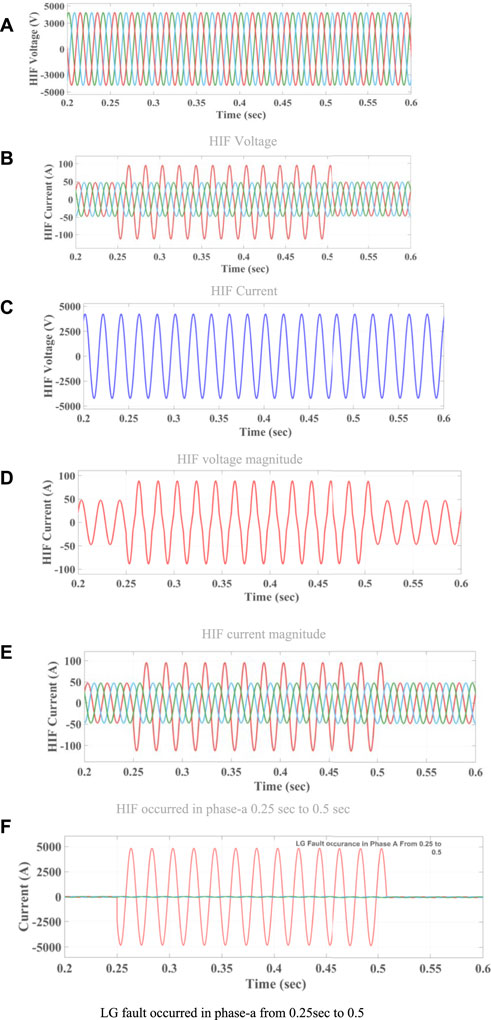
FIGURE 14. The three-phase current waveform observed for the period of 0.25–0.5 s in case of HIF fault and single line to ground (LG). (A) HIF Voltage (B) HIF Current (C) HIF voltage magnitude (D) HIF current magnitude (E) HIF occurred in phase-a 0.25 sec to 0.5 sec (F) LG fault occurred in phase-a from 0.25 sec to 0.5.

5.1 Distinguish between normal fault and no fault conditions

Table 1 describes that comparison between coefficients of phase a, b, c currents and NNRBF output of phase a, b, c and ground resistance of 20 Ω at bus 5. Conventional fault types like LG, LL, LLG, and both LLLG and HIF occurrence are used here.

TABLE 1

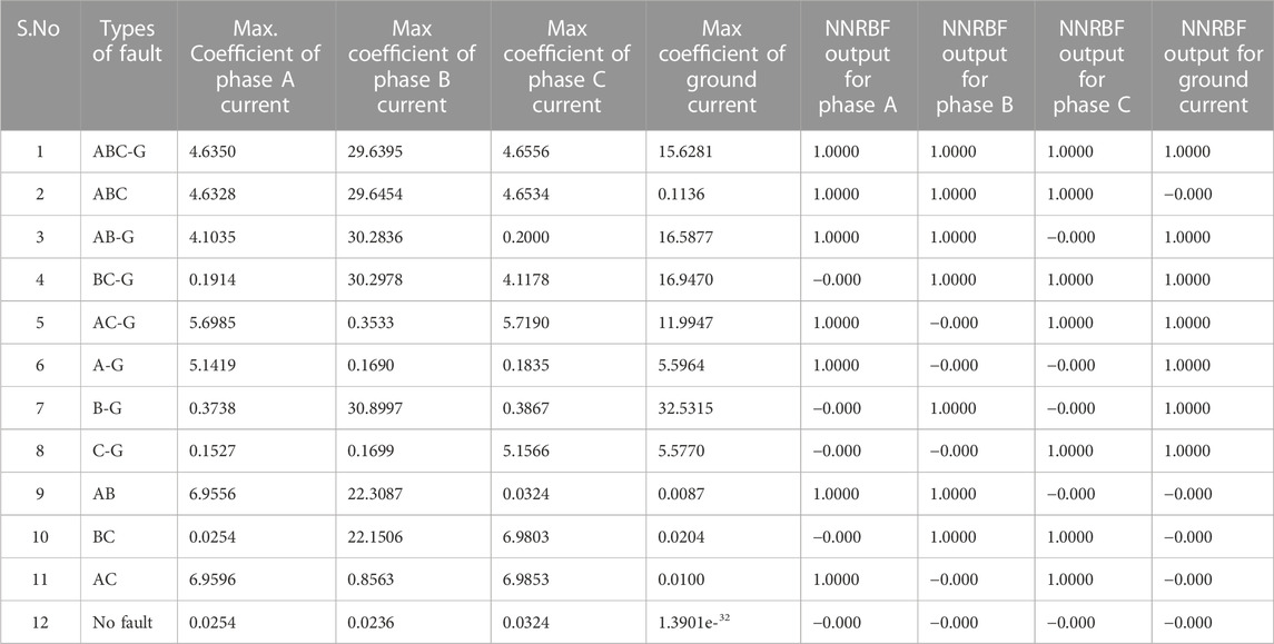
TABLE 1. Ground resistance 20 Ω detection at 5th bus.

Table 2 describes that comparison between coefficients of phase a, b, c currents and NNRBF output of phase a, b, c and ground resistance of 10 Ω at bus 5. Conventional fault types like LG, LL, LLG, and both LLLG and HIF occurrence are used here. In no fault case ground current value is high at 20 Ω when compared to 10 Ω it means when resistance is high ground current value will be very low and vice versa.

TABLE 2

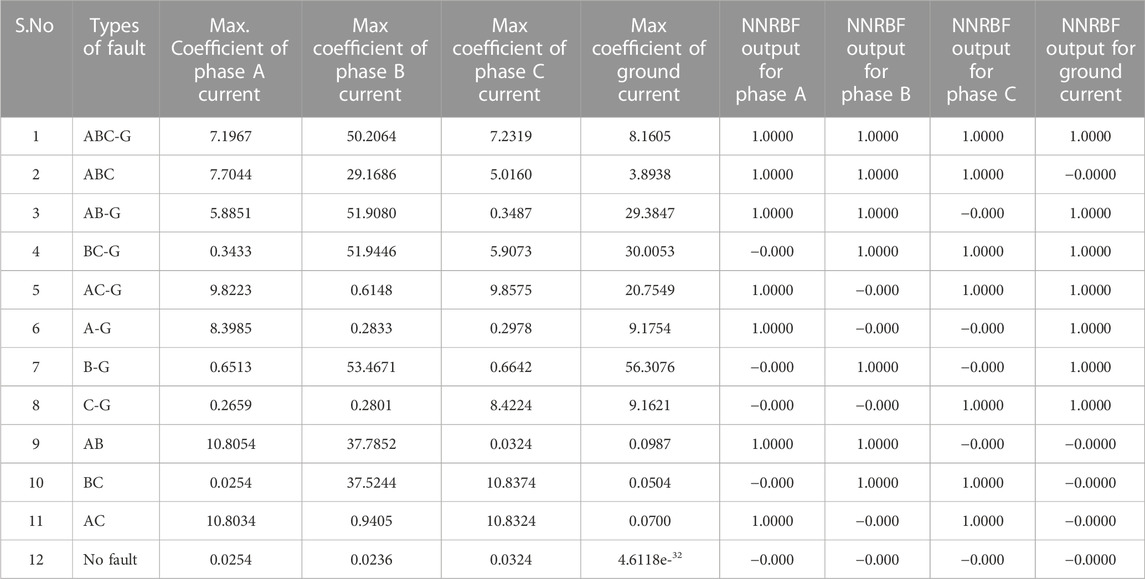
TABLE 2. Ground resistance 10 Ω location at 5th bus.

5.2 HIF voltage and current waveforms

Here, we present the simulation results for the IEEE 13-bus power network that included both PV and Wind. We simulated the PV and Wind method we intend to use to detect and identify HIF in the MV distribution network. To test the viability of the strategy, we run a MATLAB/Simulink simulation of the distribution model shown in Figure 7. In Figure 14A, we can see the time-varying current signal during the typical feeder state, which lasts for 0.25s. The HIF analysis was run alongside simulations of various power system failures to prove the viability of the proposed method. The three-phase current waveform during this time period is shown in Figure 14B in the event of an HIF fault and a single line to ground (LG). As can be seen in Figures 14C, D, the magnitude of the fault current and voltage in the case of an HIF fault in phase C of a three-phase system are small. It is shown in Figures 14E, F that if an LG fails in phase A of a three-phase system, the amplitude of the current signal is quite large, making it challenging to detect HIF in power systems. To address these issues in real time, we extracted the features using a DWT analysis, which decomposes the signal across the temporal and frequency domains. Every cycle, DWT is applied to 800 samples of the phase current signal at four different levels of decomposition. There is a different spectrum of frequencies represented by each tier; Table 1 displays the calculated SD values for each of the detailed coefficient levels and the final decomposed level (d4) (d1, d2, d3, and d4). In this paper, we present a DWT analysis of the A, B, and C stages of the system under normal conditions. Table 2 summarizes the results of the DWT analysis performed on faults with different fault resistance, such as LL, LLG, and three-phase faults, and the SD characteristics derived from these faults that were used to train classifiers to identify HIF in the system. There were 13 buses in the system, and each one had a fault applied to it so that the DWT data could be collected and used to train and test the classifiers. In this research, we used eighty percent of the data for training our classifiers and twenty percent for testing. The current setup consists of three input neurons (representing the various potential root causes of the issue) and a single output neuron (the precise count of faulty lines). Mean square error (MSE) is a common metric used to evaluate the efficacy of neural networks. All RBFNNs are considered well-trained if their MSE is less than 0.0002 and they have undergone no more than 38 training epochs. After faults are categorized, RBFNNs are put through their paces. Initial network simulation and data collection were performed in MATLAB/Simulink, covering both steady-state and transient conditions as well as the occurrence of common faults like LG, LL, LLG, and LLLG, and even HIF. As shown in Figures 14A–F, the normal operation of the power grid results in an asymmetrical current waveform due to the distribution of electrical demand.

Table 3 describes the comparison on various classification methods and % accuracy ‘$\mathrm{X}$’ represents the fault type/parameter which is not considered for classification, and ‘/’ represents the occurrence of fault.

TABLE 3

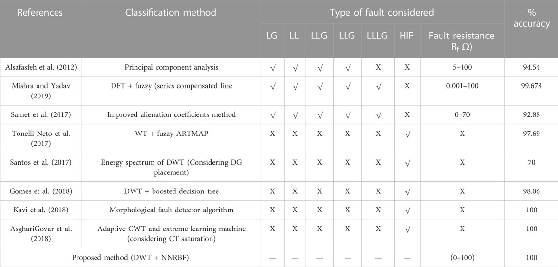
TABLE 3. Comparison on various methods.

6 Conclusion

The detection of the HIF procedure is dependent on a number of factors, some of which are unique to the characteristics of a given network. This work considers a more practical PV-integrated IEEE 13-bus system to analyze HIF using the proposed RNN-based network. Initially, a MATLAB/Simulink model of a 13-bus distribution network was built to introduce different types of events (normal operation, inrush current from a transformer, load switching, and capacitor switching, and HIF, LG, LL, LLG, and LLLG, all of which represent malfunctions in the system). Under these conditions, DWT analysis was applied to the three-phase current signal using the db4 mother wavelet. Energy value features for different phases were extracted using the obtained wavelet coefficients (d1, d2, d3, d4, d5, and a5) to train and test classifiers.

Data availability statement

The original contributions presented in the study are included in the article/Supplementary Material, further inquiries can be directed to the corresponding author.

Author contributions

VG and BE have implemented the idea and converted it into a manuscript. This idea was proposed by BE for the article “Hybrid and Neural Network Radial Basis Function Algorithms for High-Impedance Fault Detection in a Distribution Network”, and he also supervised the process. VG investigated and collected all data, wrote the draft, and converted it into an original research article.

Conflict of interest

The authors declare that the research was conducted in the absence of any commercial or financial relationships that could be construed as a potential conflict of interest.

Publisher’s note

All claims expressed in this article are solely those of the authors and do not necessarily represent those of their affiliated organizations, or those of the publisher, the editors and the reviewers. Any product that may be evaluated in this article, or claim that may be made by its manufacturer, is not guaranteed or endorsed by the publisher.

References

Abdullah, M. A., Yatim, A. H. M., and Tan, C. W. (2011). “A study of maximum power point tracking algorithms for wind energy system,” in 2011 IEEE Conference on Clean Energy and Technology (CET) (IEEE), 321–326.

CrossRef Full Text | Google Scholar

Abdullah, M. A., Yatim, A. H. M., Tan, C. W., and Saidur, R. (2012). A review of maximum power point tracking algorithms for wind energy systems. Renew. Sustain. energy Rev. 16 (5), 3220–3227. doi:10.1016/j.rser.2012.02.016

CrossRef Full Text | Google Scholar

Ahmed, J., and Salam, Z. (2018). An enhanced adaptive P&O MPPT for fast and efficient tracking under varying environmental conditions. IEEE Trans. Sustain. Energy 9 (3), 1487–1496. doi:10.1109/tste.2018.2791968

CrossRef Full Text | Google Scholar

Al-Masri, H. M., and Ehsani, M. (2015). Feasibility investigation of a hybrid on-grid wind photovoltaic retrofitting system. IEEE Trans. Ind. Appl. 52 (3), 1979–1988. doi:10.1109/TIA.2015.2513385

CrossRef Full Text | Google Scholar

Alsafasfeh, Q., Abdel-Qader, I., and Harb, A. (2012). Fault classification and localization in power systems using fault signatures and principal components analysis. Energy Power Eng. 4 (6), 506–522. doi:10.4236/epe.2012.46064

CrossRef Full Text | Google Scholar

Asghari Govar, S., Heidari, S., Seyedi, H., Ghasemzadeh, S., and Pourghasem, P. (2018). Adaptive CWT-based overcurrent protection for smart distribution grids considering CT saturation and highimpedance fault. IET Gener. Transm. Distrib. 12 (6), 1366–1373. doi:10.1049/iet-gtd.2017.0887

CrossRef Full Text | Google Scholar

Bakar, A. H. A., Ali, M. S., Tan, C., Mokhlis, H., Arof, H., and Illias, H. A. (2014). High impedance fault location in 11 kV underground distribution systems using wavelet transforms. Int. J. Electr. Power Energy Syst. 55, 723–730. doi:10.1016/j.ijepes.2013.10.003

CrossRef Full Text | Google Scholar

Bayrak, G. (2018). Wavelet transform-based fault detection method for hydrogen energy-based distributed generators. Int. J. Hydro. Energy 43 (44), 20293–20308. doi:10.1016/j.ijhydene.2018.06.183

CrossRef Full Text | Google Scholar

Billinton, R., and Karki, R. (2001). Maintaining supply reliability of small isolated power systems using renewable energy. IEE Proc. Gen. Trans. Dist. 148 (6), 530–534. doi:10.1049/ip-gtd:20010562

CrossRef Full Text | Google Scholar

Chatrenour, N., Razmi, H., and Doagou-Mojarrad, H. (2017). Improved double integral sliding mode MPPT controller based parameter estimation for a stand-alone photovoltaic system. Energy Convers. Manag. 139, 97–109. doi:10.1016/j.enconman.2017.02.055

CrossRef Full Text | Google Scholar

Chen, J., Phung, T., Blackburn, T., Ambikairajah, E., and Zhang, D. (2016). Detection of high impedance faults using current transformers for sensing and identification based on features extracted using wavelet transform. IET Gener. Transm. Distrib. 10 (12), 2990–2998. doi:10.1049/iet-gtd.2016.0021

CrossRef Full Text | Google Scholar

Costa, F. B., Souza, B. A., Brito, N. S. D., Silva, J. A. C. B., and Santos, W. C. (2015). Real-time detection of transients induced by high-impedance faults based on the boundary wavelet transform. IEEE Trans. Industry Appl. 51 (6), 5312–5323. doi:10.1109/tia.2015.2434993

CrossRef Full Text | Google Scholar

Daubecheis, I. (1992). Ten lectures on wavelets, Vol. 61. Philadelphia: SIAM.

Google Scholar

De Brito, M. A. G., Galotto, L., Sampaio, L. P., e Melo, G. D. A., and Canesin, C. A. (2012). Evaluation of the main MPPT techniques for photovoltaic applications. IEEE Trans. Indust. Electron. 60 (3), 1156–1167. doi:10.1109/tie.2012.2198036

CrossRef Full Text | Google Scholar

Elkalashy, N. I., Lehtonen, M., Darwish, H. A., Taalab, A. I., and Izzularab, M. A. (2008). “Operation evaluation of DDWT-based Earth fault detection in unearthed MV networks,” in 2008 12th International Middle-East Power System Conference (IEEE), 208–212.

Google Scholar

Emanuel, A. E., Cyganski, D., Orr, J. A., Shiller, S., and Gulachenski, E. M. (1990). High impedance fault arcing on sandy soil in 15 kV distribution feeders: Contributions to the evaluation of the low frequency spectrum. IEEE Trans. Power Deliv. 5 (2), 676–686. doi:10.1109/61.53070

CrossRef Full Text | Google Scholar

Gafoor, S. A., Yadav, S. K., and Prashanth, P. (2014). “Transmission line protection scheme using wavelet based alienation coefficients,” in Proceedings of the IEEE International Conference Power and Energy, Kyiv, Ukraine, 32–36.

CrossRef Full Text | Google Scholar

Gautam, S., and Brahma, S. M. (2012). Detection of high impedance fault in power distribution systems using mathematical morphology. IEEE Trans. Power Syst. 28 (2), 1226–1234. doi:10.1109/tpwrs.2012.2215630

CrossRef Full Text | Google Scholar

Ghaderi, A., Mohammadpour, H. A., Ginn, H. L., and Shin, Y. J. (2014). High-impedance fault detection in the distribution network using the time-frequency-based algorithm. IEEE Trans. Power Deliv. 30 (3), 1260–1268. doi:10.1109/tpwrd.2014.2361207

CrossRef Full Text | Google Scholar

Gite, S. S., and Pawar, S. H. (2017). “Modeling of wind energy system with MPPT control for DC microgrid,” in 2017 second international conference on electrical, computer and communication technologies (ICECCT) (IEEE), 1–6.

CrossRef Full Text | Google Scholar

Gomes, D. P. S., Ozansoy, C., and Ulhaq, A. (2018). High-sensitivity vegetation high-impedance fault detection based on signals highfrequency contents. IEEE Trans. Power Deliv. 33 (3), 1398–1407. doi:10.1109/tpwrd.2018.2791986

CrossRef Full Text | Google Scholar

He, Z.-Y., Liao, K., Li, X.-P., Lin, S., Yang, J.-W., and Mai, R.-K. (2014). Natural frequency-based line fault location in HVDC lines. IEEE Trans. Power Deliv. 29 (2), 851–859. doi:10.1109/tpwrd.2013.2269769

CrossRef Full Text | Google Scholar

James, J. Q., Hou, Y., Lam, A. Y., and Li, V. O. (2017). Intelligent fault detection scheme for microgrids with wavelet-based deep neural networks. IEEE Trans. Smart Grid 10 (2), 1694–1703.

Google Scholar

Jiang, J. A., Fan, P. L., and Chen, C. S. (2003). A fault detection and faulted phase selection approach for transmission lines with haar wavelet transform. IEEE PES Transm. Distribution Conf. Expo. 1 (1), 285–289.

Google Scholar

Kavaskar, S., and Mohanty, N. K. (2019). Detection of high impedance fault in distribution networks. Ain Shams Eng. J. 10 (1), 5–13. doi:10.1016/j.asej.2018.04.006

CrossRef Full Text | Google Scholar

Kavi, M., Mishra, Y., and Vilathgamuwa, M. D. (2018). High-impedance fault detection and classification in power system distribution networks using morphological fault detector algorithm. IET Gener. Transm. Distrib. 12 (15), 3699–3710. doi:10.1049/iet-gtd.2017.1633

CrossRef Full Text | Google Scholar

Kordestani, M., Safavi, A. A., and Sadrzadeh, A. (2016). “A new method to diagnose the type and location of disturbances in fars power distribution system,” in Proceedings of the 24th Iranian Conference on Electrical Engineering ICEE, Shiraz, Iran (IEEE), 1871–1876.

CrossRef Full Text | Google Scholar

Kroposki, B., Johnson, B., Zhang, Y., Gevorgian, V., Denholm, P., Hodge, B. M., et al. (2017). Achieving a 100% renewable grid: Operating electric power systems with extremely high levels of variable renewable energy. IEEE Power energy Mag. 15 (2), 61–73. doi:10.1109/mpe.2016.2637122

CrossRef Full Text | Google Scholar

Mahari, A., and Seyedi, H. (2015). High impedance fault protection in transmission lines using a WPT-based algorithm. Int. J. Electr. Power & Energy Syst. 67, 537–545. doi:10.1016/j.ijepes.2014.12.022

CrossRef Full Text | Google Scholar

Manwell, J. F., McGowan, J. G., and Rogers, A. L. (2010). Wind energy explained: Theory, design and application. John Wiley & Sons.

Google Scholar

Mishra, M., and Panigrahi, R. R. (2019). Taxonomy of high impedance fault detection algorithm. Measurement 148, 106955. doi:10.1016/j.measurement.2019.106955

CrossRef Full Text | Google Scholar

Mishra, P. K., and Yadav, A. (2019). Combined DFT and fuzzy based faulty phase selection and classification in a series compensated transmission line. Modell. Simul. Eng. 2019, 1–18. doi:10.1155/2019/3467050

CrossRef Full Text | Google Scholar

Necaibia, S., Kelaiaia, M. S., Labar, H., and Necaibia, A. (2017). Implementation of an improved incremental conductance MPPT control based boost converter in photovoltaic applications. Int. J. Emerg. Electr. Power Syst. 18 (4). doi:10.1515/ijeeps-2017-0051

CrossRef Full Text | Google Scholar

Nurzaman, I., Harini, B. W., Avianto, N., and Yusivar, F. (2017). “Implementation of maximum power point tracking algorithm on wind turbine generator using perturb and observe method,” in 2017 International Conference on Sustainable Energy Engineering and Application (ICSEEA) (IEEE), 45–51.

CrossRef Full Text | Google Scholar

Qazi, A., Hussain, F., Rahim, N. A., Hardaker, G., Alghazzawi, D., Shaban, K., et al. (2019). Towards sustainable energy: A systematic review of renewable energy sources, technologies, and public opinions. IEEE access 7, 63837–63851. doi:10.1109/access.2019.2906402

CrossRef Full Text | Google Scholar

Rezaei, N., and Haghifam, M. R. (2008). Protection scheme for a distribution system with distributed generation using neural networks. Int. J. Electr. Power Energy Syst. 30, 235–241. doi:10.1016/j.ijepes.2007.07.006

CrossRef Full Text | Google Scholar

Samantaray, S. R., Panigrahi, B. K., and Dash, P. K. (2008). High impedance fault detection in power distribution networks using time–frequency transform and probabilistic neural network. IET generation, Transm. distribution 2 (2), 261–270. doi:10.1049/iet-gtd:20070319

CrossRef Full Text | Google Scholar

Samet, H., Shabanpour-Haghighi, A., and Ghanbari, T. (2017). A fault classification technique for transmission lines using an improved alienation coefficients technique. Int. Trans. Electr. Energ Syst. 27, 22355–e2323. doi:10.1002/etep.2235

CrossRef Full Text | Google Scholar

Santos, W. C., Lopes, F. V., Brito, N. S. D., and Souza, B. A. (2016). High-impedance fault identification on distribution networks. IEEE Trans. Power Deliv. 32 (1), 23–32. doi:10.1109/tpwrd.2016.2548942

CrossRef Full Text | Google Scholar

Santos, W. C., Lopes, F. V., Brito, N. S. D., and Souza, B. A. (2017). High impedance fault identification on distribution networks. IEEE Trans. Power Deliv. 32 (1), 23–32. doi:10.1109/tpwrd.2016.2548942

CrossRef Full Text | Google Scholar

Sarlak, M., and Shahrtash, S. M. (2011). High impedance fault detection using combination of multi-layer perceptron neural networks based on multi-resolution morphological gradient features of current waveform. IET generation, Transm. distribution 5 (5), 588–595. doi:10.1049/iet-gtd.2010.0702

CrossRef Full Text | Google Scholar

Sedighi, A. R., Haghifam, M. R., Malik, O. P., and Ghassemian, M. H. (2005a). High impedance fault detection based on wavelet transform and statistical pattern recognition. IEEE Trans. Power Deliv. 20 (4), 2414–2421. doi:10.1109/tpwrd.2005.852367

CrossRef Full Text | Google Scholar

Sedighi, A. R., Haghifam, M. R., and Malik, O. P. (2005b). Soft computing applications in high impedance fault detection in distribution systems. Electr. Power Syst. Res. 76 (1-3), 136–144. doi:10.1016/j.epsr.2005.05.004

CrossRef Full Text | Google Scholar

Sekar, K., and Mohanty, N. K. (2017). Combined mathematical morphology and data mining based high impedance fault detection. Energy Procedia 117, 417–423. doi:10.1016/j.egypro.2017.05.161

CrossRef Full Text | Google Scholar

Soualhi, A., Medjaher, K., and Zerhouni, N. (2015). Bearing health monitoring based on hilbert-huang transform, support vector machine, and regression. IEEE Trans. Instrum. Meas. 64 (1), 52–62. doi:10.1109/tim.2014.2330494

CrossRef Full Text | Google Scholar

Tonelli-Neto, M. S., Decanini, J. G. M. S., Lotufo, A. D. P., and Minussi, C. R. (2017). Fuzzy based methodologies comparison for high-impedance fault diagnosis in radial distribution feeders. IET Gener. Transm. Distrib. 11 (6), 1557–1565. doi:10.1049/iet-gtd.2016.1409

CrossRef Full Text | Google Scholar

Vas, P. (1999). Sensorless vector and direct torque control. Oxford University Press.

Google Scholar

Wang, B., Geng, J., and Dong, X. (2016). High-impedance fault detection based on nonlinear voltage–current characteristic profile identification. IEEE Trans. Smart Grid 9 (4), 3783–3791. doi:10.1109/tsg.2016.2642988

CrossRef Full Text | Google Scholar

Xiao, W., Elnosh, A., Khadkikar, V., and Zeineldin, H. (2011). “Overview of maximum power point tracking technologies for photovoltaic power systems,” in IECON 2011 - 37th Annual Conference of the IEEE Industrial Electronics Society, Melbourne, VIC, 3900–3905.

CrossRef Full Text | Google Scholar

Yahya, M. G., and Yahya, M. G. (2023). Modified PDPWM control with MPPT algorithm for equal power sharing in cascaded multilevel inverter for standalone PV system under partial shading. Int. J. Power Electron. Drive Syst. 14 (1), 533. doi:10.11591/ijpeds.v14.i1.pp533-545

CrossRef Full Text | Google Scholar

Yu, L., Lai, K. K., and Wang, S. (2008). Multistage RBF neural network ensemble learning for exchange rates forecasting. Neurocomputing 71 (16-18), 3295–3302. doi:10.1016/j.neucom.2008.04.029

CrossRef Full Text | Google Scholar

Zayandehroodi, H., Mohamed, A., Shareef, H., and Mohammadjafari, M. (2010). “Performance comparison of MLP and RBF neural networks for fault location in distribution networks with DGs,” in IEEE International Conference on Power and Energy (PECon 2010), Kuala Lumpur, Malaysia, 341–345.

CrossRef Full Text | Google Scholar

Zayandehroodi, H., Mohamed, A., Shareef, H., and Mohammadja, M. (2010). Automated Fault location in a power system with distributed generations using radial basis function neural networks. Int. J. Appl. Sci. 10, 3032–3041. doi:10.3923/jas.2010.3032.3041

CrossRef Full Text | Google Scholar