A combined model based on secondary decomposition technique and grey wolf optimizer for short-term wind power forecasting

Short-term wind power forecasting plays an important role in wind power generation systems. In order to improve the accuracy of wind power forecasting, many researchers have proposed a large number of wind power forecasting models. However, traditional forecasting models ignore data preprocessing and the limitations of a single forecasting model, resulting in low forecasting accuracy. Aiming at the shortcomings of the existing models, a combined forecasting model based on secondary decomposition technique and grey wolf optimizer (GWO) is proposed. In the process of forecasting, firstly, the complete ensemble empirical mode decomposition adaptive noise (CEEMDAN) and wavelet transform (WT) are used to preprocess the wind power data. Then, least squares support vector machine (LSSVM), extreme learning machine (ELM) and back propagation neural network (BPNN) are established to forecast the decomposed components respectively. In order to improve the forecasting performance, the parameters in LSSVM, ELM, and BPNN are tuned by GWO. Finally, the GWO is used to determine the weight coefficient of each single forecasting model, and the weighted combination is used to obtain the final forecasting result. The simulation results show that the forecasting model has better forecasting performance than other forecasting models.

1 Introduction

As a clean and pollution-free renewable resource, wind energy has attracted much attention because of its abundant resources, wide distribution and great development potential (Hua et al., 2022; Khazaei et al., 2022). However, due to the intermittent and strong variability of wind power (Yin et al., 2021; Duan et al., 2022). Therefore, it is necessary to develop a method that can accurately forecast wind power, reduce the negative impact of wind power grid connection, ensure the safe and stable operation of the power system, and improve the utilization rate of wind power in the power system (Hu et al., 2021a; Lin and Zhang, 2021; Meng et al., 2022).

In recent years, many scholars have done a lot of research in the field of wind power forecasting, and proposed many wind power forecasting methods. These forecasting methods can be divided into three categories: physical methods and general statistical methods and artificial intelligence methods (Xiang et al., 2019; Zhang et al., 2019; Hu et al., 2021b). Physical methods does not need the support of historical data, its principle is to use the wind speed, wind direction and temperature of numerical weather forecasting information as input data, and then combined with the surface information around the fan to establish a mathematical model for solving (Du et al., 2017). The calculation process of physical method is complicated and the cost is high, so it is suitable for long-term forecasting, and the error is large in short-term wind power forecasting (Soman et al., 2010; Zhang et al., 2020). In contrast, general statistical methods and artificial intelligence methods only need to use historical wind power data for wind power forecasting, which is easy to implement and more suitable for short-term wind power forecasting (Tascikaraoglu and Uzunoglu, 2014; Zhou et al., 2022). General statistical methods mainly include the autoregression (AR) method (Huang and Chalabi, 1995), the autoregressive moving average (ARMA) method (Erdem and Shi, 2011) and grey models (GM) method (Bahrami et al., 2014). Artificial intelligence technology has outstanding advantages in dealing with non-linear problems, and many researchers have applied artificial intelligence methods to the field of wind power forecasting (Ogliari et al., 2021; Wang et al., 2021; Chen et al., 2022a). Artificial intelligence methods mainly include BP neural network (BPNN) (Zhu et al., 2022), support vector machine (SVM) (Li et al., 2020)^, extreme learning machine (ELM) (Peng et al., 2017), generalized regression neural network (GRNN) (Ding et al., 2021) and Long-term and Short-term Memory network (LSTM) (Xiong et al., 2022) etc. Ren et al. (Ren et al., 2014) proposed an IS-PSO-BP wind speed forecasting model, which achieved good forecasting performance. Liao et al. (Liao et al., 2021) introduces fuzzy seasonal index into fuzzy LSTM model has better performance in terms of forecasting accuracy.

In the past few decades, researchers have proposed many wind power forecasting methods, which have improved the wind power forecasting accuracy to a certain extent. However, considering the non-stationarity of wind power data, direct use of raw data for forecasting will lead to large errors. The usual method is to use empirical mode decomposition (EMD), ensemble empirical mode decomposition (EEMD) and wavelet transform (WT). Zhang et al. (Zhang et al., 2017) proposed an EEMD combined with cuckoo search optimization algorithm to optimize the wavelet neural network for wind speed forecasting and the experiments show that EEMD can make a great contribution to the forecasting accuracy. Liu et al. (Liu et al., 2014) proposed a wind speed forecasting model based on wavelet transform and genetic algorithm to optimize support vector machine. Wavelet transform can eliminate the random fluctuation of wind speed sequence and improve the accuracy of wind speed forecasting.

The limitations of the above methods are summarized as follows:

1) Physical methods are suitable for long-term forecasting rather than short-term forecasting.

2) General statistical methods are suitable for linear data, but not for non-linear data; A single artificial intelligence forecasting method is difficult to get rid of the problems of local optima and low convergence.

3) The traditional single data processing method cannot completely solve the non-linear and non-stationary components of the original wind power data.

4) The limitations of a single forecasting model make it difficult to ensure accurate forecasting for all wind power datasets.

Based on the analysis above, a developed combined wind power forecasting model that is based on the complete ensemble empirical model decomposition adaptive noise (CEEMDAN) and wavelet transform (WT) secondary decomposition technique (SDT), grey wolf optimizer (GWO) and three individual forecasting models. First, CEEMDAN is used to process wind power data, and WT is used for secondary decomposition of the most complex IMF1 component. Then the forecasting models of GWO-LSSVM, GWO-ELM and GWO-BPNN are established. Finally, a weight optimization method based on GWO algorithm is developed to combine the results of three individual forecasting models to obtain the final forecasting results.

The primary contributions and innovations of this study are described as follows:

1) CEEMDAN is used to process the wind power series, and WT is used to decompose the IMF1 component with the highest complexity, which effectively reduces the volatility and non-stationarity of wind power data and improves the forecasting performance.

2) Three machine learning methods LSSVM, ELM and BPNN are proposed to forecast the processed wind power. In order to improve the forecasting accuracy, GWO algorithm is used to optimize the hyperparameters of these three machine learning models.

3) A weight determination method of combined forecasting model based on GWO algorithm is proposed to find the weight of each individual forecasting model.

4) The novel combined forecasting model based on three individual machine learning models effectively utilizes the advantages of each individual forecasting model and improves the forecasting accuracy of short-term wind power.

The structure of this paper will be described in detail below. Section 2 introduces data preprocessing methods and the principles of three machine learning forecasting models. Section 3 introduces the principle of the optimization algorithm and the process of building a combined forecasting model. Section 4 presents the dataset sources, performance evaluation metrics, and testing methods of this study, and the comparison results of the proposed model and other models are analyzed in detail in Section 4 to verify the forecasting performance of the combined forecasting model. Finally, Section 5 presents the research conclusions of this paper. The main terminologies mentioned in this paper are show in Table 1.

TABLE 1

TABLE 1. The main terminologies mentioned in this paper.

2 Methodology

2.1 CEEMDAN

EMD is a method for processing non-stationary signals. The signal is decomposed into IMFs of different frequencies through a screening process. The EMD method has the disadvantage of modal mixing and cannot accurately extract the effective feature information of the signal (Hu et al., 2013). In order to solve the modal mixing problem of EMD decomposition, the EEMD method is to add a Gaussian white noise to the sample data during the EMD decomposition process, and eliminate these noise signals by averaging (Hu et al., 2013; Nguyen and Phan, 2022). However, after limited iterations, the reconstructed signal still contains a noisy signal. In order to eliminate residual noise, Torres et al. proposed to add adaptive auxiliary noise signals in the process of EMD decomposition. Compared with EMD and EEMD, this method effectively eliminated the problem of mode mixing (Chen et al., 2022b). The decomposition steps of CEEMDAN are as follows:

Step1: Assuming $x\left(t\right)$ that is the original wind power data, add Gaussian white noise to the original signal.

$y\left(t\right)=x\left(t\right)+{\eta }_{0}z\left(t\right)(1)$

Where ${\eta }_0$ denotes a noise coefficient.

Step2: Signal $y\left(t\right)$ is repeatedly decomposed for L times, and then the mean is calculated to obtain the

First IMF of CEEMDAN.

$IM{F}_1\left(t\right)=\frac{1}{L}{\displaystyle \sum }_{i=1}^{L}IM{F}_1^i\left(t\right)(2)$

Step3: Calculate residuals $r_1\left(t\right)$.

$r_1\left(t\right)=x\left(t\right)-IM{F}_1^i\left(t\right)(3)$

Step4: Use EMD to decompose signal $r_1\left(t\right)+{\eta }_1{E}_1\left(z\left(t\right)\right)$ and calculate the second IMF.

$IM{F}_2^i(t)=\frac{1}{L}{\displaystyle \sum }_{i=1}^L\left.E_1(r_1(t)+{\eta }_1{E}_1(z(t)\right))(4)$

Where $E_1\left(\right)$ represents EMD decomposition.

Step5: Calculate the k_th residual component.

$r_k\left(t\right)=r_{k-1}\left(t\right)-IM{F}_k^i\left(t\right)k=2,3,\cdots ,L(5)$

Step6: Repeat the calculation process of step 4 to obtain the k_th IMF.

$IM{F}_k=\frac{1}{L}{\displaystyle \sum }_{i=1}^L\left.E_1(r_k(t)+{\eta }_k{E}_k(z(t)\right))(6)$

Step7: Finally, the decomposition result is as follows.

$p\left(t\right)=r_k\left(t\right)+\frac{1}{L}{\displaystyle \sum }_{i=1}^{L}IM{F}_1^i\left(t\right)(7)$

2.2 WT

Wavelet transform is a data decomposition method, which has been successfully applied in various fields, including image processing, signal denoising and time series analysis (Bento et al., 2019). Wavelet transforms can be classified into two categories: continuous wavelet transform (CWT) and discrete wavelet transform (DWT). The CWT causes a large amount of computation because of repeated calculation, and the DWT has better computational efficiency. Therefore, this paper uses the DWT to process wind power data. The three-layer decomposition of wind power data by discrete wavelet transform is shown in Figure 1. The original signal is broken into two components by high-pass filter (HPF) and low-pass filter (LPF), namely approximation component ($A_i$) and detail component ($D_i$). Then, the approximation component is decomposed by the second layer to obtain the approximation component and detail component, and so on to obtain the third-layer decomposition.

$DWT\left(a,b\right)={\displaystyle \sum }_{t=0}^{T-1}x\left(t\right)\psi \left(\frac{t-b\cdot 2^a}{2^a}\right)(8)$

Where T is the total length of the original signal $x\left(t\right)$, a and b are the scaling and translation parameters respectively and t is discrete time.

FIGURE 1

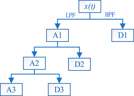
FIGURE 1. Three-level decomposition of signal by WT.

2.3 LSSVM

The least squares support vector machine is an improved algorithm based on the support vector machine. The principle is to map the data to a high-dimensional space through a non-linear function and perform linear regression (Zhang and Li, 2022). The established regression function is:

$y=w^T\cdot \phi \left(x\right)+b(9)$

Where w is the weight vector, b is the bias term.

According to the principle of structural risk minimization, the objective function can be expressed as:

$\min J\left(w,e\right)=\frac{1}{2}{w}^{T}w+\frac{1}{2}\gamma {\displaystyle \sum }_{i=1}^n{e}_i^2(10)$

Such that:

$y_i=w^T\cdot \phi \left(x_i\right)+b+e_i,i=\mathrm{1,2},...,n(11)$

Where $\gamma$ is error penalty function, $e_i$ is slack variable.

Construct the Lagrange function L:

$L\left(w,b,e,\alpha \right)=\frac{1}{2}{w}^{T}w+\frac{1}{2}\gamma {\displaystyle \sum }_{i=1}^N{e}_i^2-{\displaystyle \sum }_{i=1}^N{\alpha }_i\{w^T\phi \left(x_i\right)+b+e_i-y_i\}(12)$

Where ${\alpha }_i$ is the Lagrangian multiplier.

According to KKT conditions:

$\left\{\begin{array}{l}\frac{\partial L}{\partial w}=0\to w={\displaystyle \sum }_{i=1}^n{\alpha }_i{y}_i\phi \left(x_i\right)\\ \frac{\partial L}{\partial b}=0\to {\displaystyle \sum }_{i=1}^n{\alpha }_i=0\\ \frac{\partial L}{\partial e_i}=0\to {\alpha }_i=\gamma e_i\\ \frac{\partial L}{\partial {\alpha }_i}=0\to w^T\phi \left(x_i\right)+b+e_i-y_i=0\end{array}\right.(13)$

After eliminating w and e, the linear equations can be obtained as follows:

$\left[\begin{array}{cc}0& I^T\\ I& Z{Z}^T+\frac{I}{\gamma }\end{array}\right]\left[\begin{array}{c}b\\ \alpha \end{array}\right]=\left[\begin{array}{c}0\\ y\end{array}\right](14)$

Where$Z=\left[\varphi {\left(x_1\right)}^T{y}_1,\cdots ,\varphi {\left(x_N\right)}^T{y}_N\right]$,$I={\left[1,\cdots ,1\right]}^T$, $y={\left[y_1,\cdots ,y_N\right]}^T$, and $\alpha ={\left[{\alpha }_1,\cdots ,{\alpha }_N\right]}^T$.

According to the Mercer condition, the kernel function $k\left(x_i,x_j\right)$ is equivalent to the scalar product calculation in the above equation to linearize the non-linear problem.

$K\left(x_i,x_j\right)=\varphi {\left(x_i\right)}^T\varphi \left(x_j\right)(15)$

The LSSVM model expression is:

$y\left(x\right)={\displaystyle \sum }_{i=1}^N{\alpha }_{i}K\left(x,x_i\right)+b(16)$

The performance of LSSVM is affected by regularization parameters, kernel function types and parameters. The RBF kernel function has the advantages of good generalization ability, simple expression and wide convergence region. In this paper, the RBF kernel function is selected as the kernel function of the LSSVM model.

2.4 ELM

ELM is a kind of single-hidden layer feed forward networks (SLFNs) proposed by Huang et al., which consists of input layer, hidden layer and output layer (Huang et al., 2006). After initialization, the input weight between the input layer and the hidden layer and the bias value of the hidden layer are randomly selected, and then the output weight can be calculated according to the generalized inverse operation on the output matrix. Compared with traditional feed-forward neural networks with single hidden layer, ELM has the advantages of fast operation speed, simple structure and small error, and is widely used in many fields.

Given any N samples $\left(x_i,t_i\right)$, where the input sample is $x_i={\left[x_{i1},x_{i2},\cdots ,x_{in}\right]}^T\in R^n$, the output sample is $t_i=\left[t_{i1},t_{i2},\cdots ,t_{im}\right]\in R^m$, L is defined as the number of neurons in the hidden layer, and $g\left(x\right)$ is the activation function, the SLFNs model can be expressed as follows:

${\displaystyle \sum }_{i=1}^L{\beta }_i{g}_i\left(x_i\right)={\displaystyle \sum }_{i=1}^L{\beta }_{i}g\left(w_i\cdot w_j+b_i\right)=o_j,j=\mathrm{1,2},\cdots ,N(17)$

Where $w_i={\left[w_{i1},w_{i2},\cdots ,w_{in}\right]}^T$ is the input weight, ${\beta }_i={\left[{\beta }_{i1},{\beta }_{i2},\cdots ,{\beta }_{im}\right]}^T$ is the output weight, $b_i$ is the bias, $o_j$ is the output value of the model, and $w_i\cdot w_j$ is the inner product of $w_i$ and $w_j$.

The learning mechanism of SLFNs is realized by the zero error between the output value and the sample, expressed as ${\displaystyle \sum }_{j=1}^N‖o_j-y_j‖$, so Eq. 17 can be expressed as:

${\displaystyle \sum }_{i=1}^L{\beta }_{i}g\left(w_i\cdot w_j+b_i\right)=y_j,j=\mathrm{1,2},\cdots ,N(18)$

Eq. 18 can be expressed in matrix form as:

$H\beta =T(19)$

Where H is the hidden layer output matrix of ELM, $\beta$ is the weight matrix, and T is the network output matrix.

The hidden layer output weights can be obtained by solving the least squares solution of the following equation:

$\underset{\beta }{\min }‖H\beta -T‖(20)$

The solution is:

$\stackrel{\wedge }{\beta }=H^{+}T(21)$

Where $H^{+}$ is the Moore–Penrose generalized inverse matrix of the hidden layer output matrix.

2.5 BPNN

Back propagation neural network is a kind of multilayer feedforward neural network trained by error back propagation. BP neural network is composed of input layer, hidden layer and output layer. The hidden layer of the network can be one or more layers, each layer is composed of one or more neurons. The neurons of neighboring layers are connected to each other, and each neuron only receives the input of the neuron of the previous layer, while there is no connection between neurons of the same layer. Only the input information processed by neurons in each layer can become the output of the output layer. The training process of BP neural network is as follows:

The output of the hidden layer can be expressed as:

$H_j=g\left({\displaystyle \sum }_{i=1}^n{w}_{ij}{x}_i-a_j\right),j=\mathrm{1,2},\cdots ,l(22)$

Where l is the number of hidden layer nodes, n is the number of input layer nodes, w is the weight between the input layer and the hidden layer, x is the input variable, a is the hidden layer threshold, and $g\left(x\right)=\frac{1}{1+e^{-x}}$ is the activation function.

The output of the output layer can be expressed as:

$O_k={\displaystyle \sum }_{j=1}^l{H}_j{w}_{ik}-b_k,k=\mathrm{1,2},\cdots ,m(23)$

Where m is the number of output layer nodes, w is the weight between the hidden layer and the input layer, and b is the output layer threshold.

The forecasting error is calculated by the expected output Y minus the output O of the output layer, and the expression is:

$e_k=Y_k-O_k,k=\mathrm{1,2},\cdots ,m(24)$

From the forecasting error $e_k$, the updated expressions for the weights and thresholds can be obtained:

$w_{ij}=w_{ij}+\eta H_j\left(1-H_j\right)x\left(i\right){\displaystyle \sum }_{k=1}^m{w}_{jk}{e}_k,i=1\cdots ,n;j=1,\cdots ,l(25)$

$w_{jk}=w_{jk}+\eta H_j{e}_k,j=\mathrm{1,2},\cdots ,l;k=\mathrm{1,2},\cdots ,m(26)$

$a_j=a_j+\eta H_j\left(1-H_j\right)x\left(i\right){\displaystyle \sum }_{k=1}^m{w}_{jk}{e}_k,j=\mathrm{1,2},\cdots ,l(27)$

$b_k=b_k+e_k,k=\mathrm{1,2},\cdots ,m(28)$

Where $\eta$ is the learning rate, and $x\left(i\right)$ represents the i-th input variable.

3 Wind power forecasting model

3.1 Grey wolf optimizer

Grey wolf optimizer is a new swarm intelligence optimization algorithm. It is optimized by simulating the predation behavior of the grey wolf population and by tracking, surrounding, pursuing and attacking the wolves (Mirjalili et al., 2014)^. The algorithm has the advantages of simple principle, less parameters to be adjusted, easy implementation and strong global search ability. In recent years, researchers have applied GWO to many research fields, such as image processing (Rajput et al., 2019; Rajput and S-GWO-FH, 2022), path planning (Dong et al., 2022; Zhang et al., 2022), power scheduling and forecasting (Lu et al., 2020; Wang et al., 2020; Jalali et al., 2022), and other related fields.

The wolves are divided into four groups according to the social rank: $\alpha ,\beta ,\delta$ and $w$, $\alpha$ as the optimal solution, $\beta$ and $\delta$ as the suboptimal solution, and w is the candidate solution.

In the process of hunting, the behavior of wolves surrounding prey can be expressed as follows:

$D=\left|\overrightarrow{C}\cdot \overrightarrow{X_p}\left(t\right)-\overrightarrow{X}\left(t\right)\right|(29)$

$\overrightarrow{X}\left(t+1\right)={\overrightarrow{X}}_P\left(t\right)-\overrightarrow{A}\cdot \overrightarrow{D}(30)$

Where t is the number of current iterations, $\overrightarrow{X_p}$ is the position vector of prey, $\overrightarrow{X}$ is the position vector of grey Wolf, $\overrightarrow{A}$ and $\overrightarrow{C}$ is the coefficient vector. The expressions of $\overrightarrow{A}$ and $\overrightarrow{C}$ are:

$\overrightarrow{A}=2\overrightarrow{a}\cdot \overrightarrow{r_1}-\overrightarrow{a}(31)$

$\overrightarrow{C}=2\cdot \overrightarrow{r_2}(32)$

Where $\overrightarrow{r_1}$ and $\overrightarrow{r_2}$ are random vectors between [0,1], $\overrightarrow{a}$ is the convergence factors, and linearly decrease from 2 to 0 in the iteration process.

Suppose $\alpha ,\beta \text{and}\delta$ have a better idea of the potential location of prey. Therefore, we save the top three best solutions obtained so far and ask other grey wolf individuals to update their positions based on the location of the greyest individual. The mathematical expression of the update process is:

${\overrightarrow{D}}_{\alpha }=\left|{\overrightarrow{C}}_1\cdot {\overrightarrow{X}}_{\alpha }-\overrightarrow{X}\right|,{\overrightarrow{D}}_{\beta }=\left|{\overrightarrow{C}}_2\cdot {\overrightarrow{X}}_{\beta }-\overrightarrow{X}\right|,{\overrightarrow{D}}_{\delta }=\left|{\overrightarrow{C}}_3\cdot {\overrightarrow{X}}_{\delta }-\overrightarrow{X}\right|(33)$

${\overrightarrow{X}}_1={\overrightarrow{X}}_{\alpha }-{\overrightarrow{A}}_1\cdot \left({\overrightarrow{X}}_{\alpha }\right),{\overrightarrow{X}}_2={\overrightarrow{X}}_{\beta }-{\overrightarrow{A}}_2\cdot \left({\overrightarrow{X}}_{\beta }\right),{\overrightarrow{X}}_3={\overrightarrow{X}}_{\delta }\cdot {\overrightarrow{A}}_3\cdot \left({\overrightarrow{X}}_{\delta }\right)(34)$

$\overrightarrow{X}\left(t+1\right)=\frac{{\overrightarrow{X}}_1+{\overrightarrow{X}}_2+{\overrightarrow{X}}_3}{3}(35)$

Where t is the number of current iterations, ${\overrightarrow{C}}_1,{\overrightarrow{C}}_2,{\overrightarrow{C}}_3$, ${\overrightarrow{A}}_1,{\overrightarrow{A}}_2,{\overrightarrow{A}}_3$ are random vectors.

In the process of hunting, firstly, the distance between individuals is calculated, and then the direction of individual moving to prey is determined by the synthesis of Eq. 35, and finally the prey is captured to complete the hunting. Table 2 shows the pseudo code of GWO.

TABLE 2

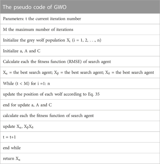
TABLE 2. The pseudo code of GWO.

3.2 Individual forecasting model

The specific steps of the forecasting model of GWO-ELM are as follows:

Step1: Initialize the number of wolves and random population positions, determine the number of hidden layer nodes and the maximum number of iterations.

Step2: Initialize the fitness value. The root mean square error (RMSE) is selected as the fitness function, and the individual fitness function value is calculated and sorted by size to select $\alpha$, $\beta$ and $\delta$ wolf.

Step3: Update the position of each wolf in the wolf pack according to Eq. 35, and calculate the fitness value at the same time.

Step4: Judge whether it meets the given convergence accuracy or the maximum number of iterations; if not, return to Step2; if yes, output the optimal solution, namely the position of $\alpha$ wolf.

Step5: According to the position of $\alpha$ wolf, the input layer weight and hidden layer threshold of extreme learning machine are obtained, and finally the forecasting model of GWO-ELM is established.

The process of GWO-LSSVM and GWO-BP forecasting models are in the similar manners.

3.3 Parameter setting

The population size of GWO set 30, and the maximum number of iterations set 50. The input layer node of ELM is 6, hidden layer node is 30 and the output layer node is 3. The input layer node of BPNN is 6, the middle layer is 8 and the output layer node is 3.

3.4 Construction of the combined model

Combined forecasting model is a kind of model which is often used in forecasting field. The key of model establishment lies in how to determine the weight coefficient of single forecasting model. By assigning corresponding weights to multiple forecasting models, the forecasting result of each single forecasting model is multiplied by its corresponding weight to obtain the forecasting result of the forecasting model. Finally, the final forecasting result is generated by adding the results of all forecasting models. The calculation process is shown in Eq. 36. (Xiao et al., 2015). proposed the theory of no negative constraint theory (NNCT) to obtain the weight coefficient.

In this study, the grey wolf optimizer is adopted, the population size set 30, the maximum number of iterations is 200, and RMSE is used as the loss function, and the optimal weight coefficient is obtained by minimizing the loss function.

$y={\displaystyle \sum }_{i=1}^n{w}_i{f}_i(36)$

Where y is the forecasting result of the combined forecasting model, $f_i$ is the forecasting result of the single forecasting model, and w is the weight coefficient.

The strategy of combined forecasting model is shown in Figure 2, and the process of combining forecasting model is as follows:

FIGURE 2

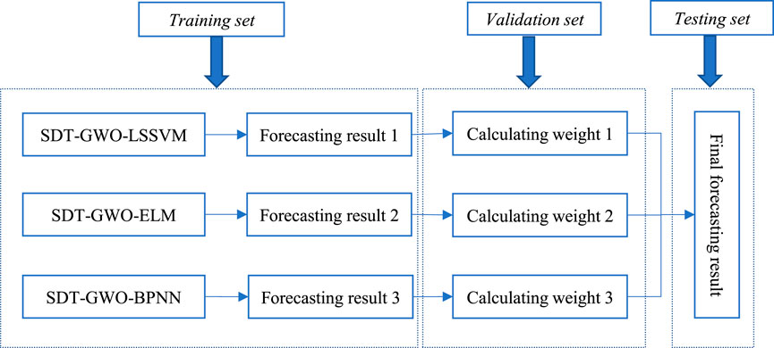
FIGURE 2. Combined forecasting model strategy.

Stage1: Data pretreatment.

Aiming at the problem that forecasting model based on single decomposition technology can not completely deal with the non-linearity and non-stationarity of wind power series, a secondary decomposition technique based on the combination of CEEMDAN and WT is proposed in this study.

Stage2: Forecasting model.

Three machine learning models with good forecasting performance, LSSVM, ELM and BPNN, are selected for wind power forecasting, and the GWO algorithm is used to optimize the hyperparameters of these three machine learning models to further improve the forecasting accuracy. The data pretreatment results in Stage1 are combined with the three forecasting models to forecast wind power, and the process is shown in Figure 3. The two datasets selected in this study are both 1248 data points, among which the first 960 data points are training data sets and the second 288 data points are validation and testing data sets. The first 960 data points are input into the forecasting model and 288 data points are output. The input and output matrix format of multi-step forecasting in this paper is shown in Figure 4.

FIGURE 3

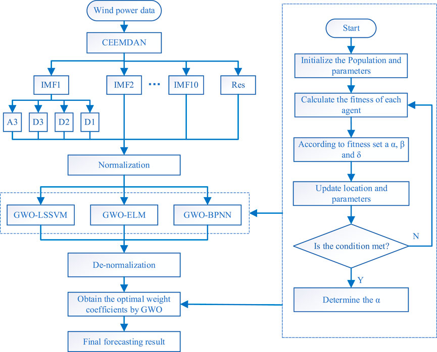
FIGURE 3. Framework of the proposed forecasting model.

FIGURE 4

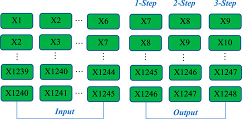
FIGURE 4. Input and output matrix format for combined model.

Stage3: Calculate the weight of combined forecasting model.

In order to better calculate the weight coefficient of combined forecasting model, a weight determination method of combined forecasting model based on GWO algorithm is proposed. Firstly, 288 data points obtained from Stage2 are selected, among which the first 192 data points are the validation dataset to determine the weight of the combined forecasting model, and the last 96 data points are the testing dataset. The dimension of GWO is set as 3, the number of iterations is set as 200, and the upper and lower limits of weight are set as [-2,2] to obtain the optimal weight coefficient. According to Eq. 36, the final wind power forecasting result can be calculated.

4 Experiments and analysis

All simulation experiments are carried out on MATLAB R2020b environment in a personal computer with i7-10750H CPU and 16 GB RAM.

4.1 Data description

In this study, historical wind power data are used from the Belgian electricity operator Elia, which can be downloaded from its website (Elia Transmission Company, 2021). Two sets of 13-day wind power data are randomly selected from 2019 with a sampling interval of 15min. Each set contained 1248 data points and illustrated in Figure 5 and the samples of the first 10 days of each dataset are used as the training dataset, the samples of the first 2 days of the next 3 days are used as the validation dataset to determine the weight of each model, and the samples of the last 1 day are used as the test dataset to evaluate the prediction effect of the combined model. The statistical description of wind power data is shown in Table 3.

FIGURE 5

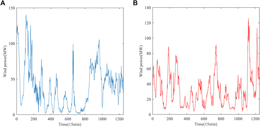
FIGURE 5. The original wind power series. (A) Wind power of dataset A. (B) Wind power of dataset B.

TABLE 3

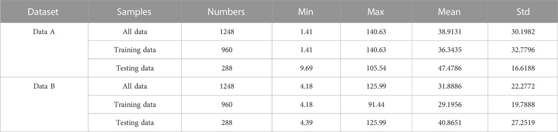
TABLE 3. Statistical characteristic of two datasets.

4.2 Secondary decomposition technique

In this study, the secondary decomposition technique is used to preprocess the original wind power to reduce the non-stationarity of the wind power series. Firstly, the wind power series is decomposed into different IMF components and a residual component Res by CEEMDAN technology, as shown in Figure 6. Secondly, the highly complex IMF1 component was decomposed by wavelet. At this stage, IMF1 was decomposed into four components, namely A3, D3, D2 and D1, which further reduced the volatility and non-stationary of IMF1 component, as shown in Figure 7. In the experiment, the parameters of CEEMDAN and WT is set as follows: Nstd value is 0.2, NR value is 500, the maximum number of iterations is 5000, and db5 as the wavelet function.

FIGURE 6

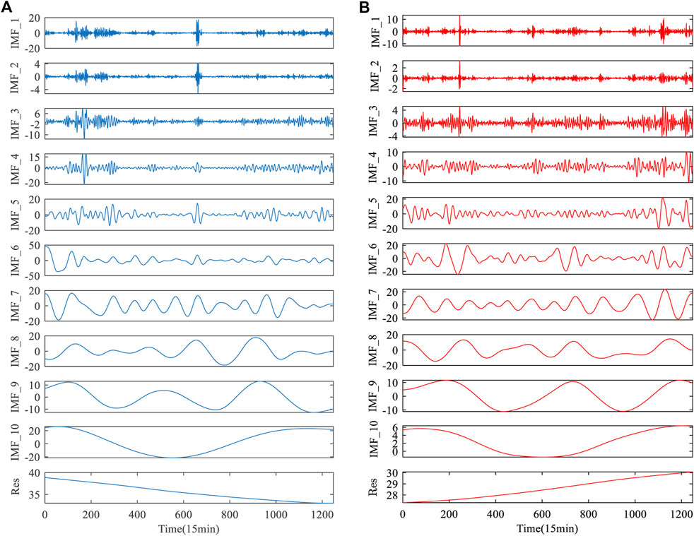
FIGURE 6. Decomposition results of wind power by CEEMDAN. (A) Wind power of dataset A. (B) Wind power of dataset B.

FIGURE 7

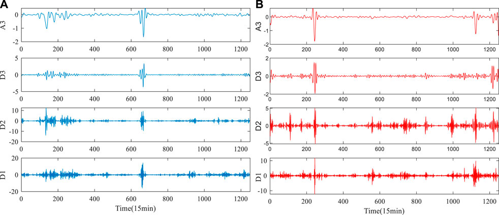
FIGURE 7. Decomposition results of IMF1 by WT. (A) Wind power of dataset A. (B) Wind power of dataset B.

4.3 Evaluation criteria

The evaluation criteria of the forecasting method are used to test the accuracy of the forecasting model. The smaller the value of the evaluation criteria, the better the forecasting performance of the model. In this study, the evaluation criteria are selected as root mean square error (RMSE), mean absolute error (MAE), mean absolute percentage error (MAPE) and square sum of the error (SSE). The expressions are as follows:

$MAE=\frac{1}{N}{\displaystyle \sum }_{i=1}^N\left|Y_{Ai}-Y_{Fi}\right|(37)$

$RMSE=\sqrt{\frac{1}{N}{\displaystyle \sum }_{i=1}^N{\left(Y_{Ai}-Y_{Fi}\right)}^2}(38)$

$MAPE=\frac{1}{N}{\displaystyle \sum }_{i=1}^N\frac{\left|Y_{Ai}-Y_{Fi}\right|}{Y_{Ai}}\times 100\%(39)$

$SSE={\displaystyle \sum }_{i=1}^N{\left(Y_{Ai}-Y_{Fi}\right)}^2(40)$

Where N is the number of samples, $Y_{Ai}$ is the true value of wind power, and $Y_{Fi}$ is the forecasting value of wind power.

4.4 Experiment description

Based on the historical wind power, four experiments are established in this paper, and the combined model established is compared with other forecasting models through these four groups of experiments.

4.4.1 Experiment 1

Experiment 1 includes four forecasting models, including SDT-GWO-LSSVM, SDT-GWO-ELM, SDT-GWO-BPNN and Proposed Model. Figure 8 is the comparison of forecasting results of dataset A in Experiment 1, and Figure 9 is the comparison of forecasting results of dataset B in Experiment 1. The pair of evaluation criteria results of Experiment 1 is shown in Table 4, in which the bold part is the forecasting result of Proposed Model.

FIGURE 8

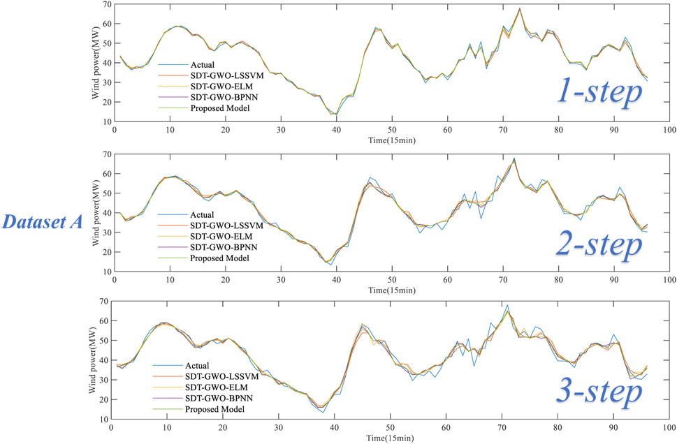
FIGURE 8. Comparison of the multi-step forecasting performance of Experiment 1 for dataset A.

FIGURE 9

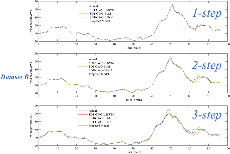
FIGURE 9. Comparison of the multi-step forecasting performance of Experiment 1 for dataset B.

TABLE 4

TABLE 4. Forecasting performance results of each model in Experiment 1.

For dataset A, whether it is 1-step or multi-step prediction, the proposed combination forecasting model has excellent performance, and its 1-step, 2-step and 3-step MAPE values are 1.972%, 3.630% and 4.456%, respectively, with the smallest error compared with other prediction models. Taking the three-step prediction results as an example, the MAPE value of the Proposed model de-creased by 0.366%, 0.194% and 0.097% respectively compared with SDT-GWO-LSSVM, SDT-GWO-ELM and SDT-GWO-BPNN.

For dataset B, the proposed model has superior prediction effect. The MAPE values of the 1-step, the 2-step and 3-step are 1.325%%, 2.693% and 3.538% respectively, which has the smallest error compared with other pre-diction models. Taking the 3-step prediction results as an example, the MAPE value of The Proposed model is reduced by 0.333%, 0.463% and 0.205% compared with SDT-GWO-LSSVM, SDT-GWO-ELM and SDT-GWO-BPNN, respectively.

4.4.1.1 Remark

Through the analysis of the prediction results in Experiment 1, no matter dataset A and dataset B, the three single prediction models have good prediction performance. The proposed model combines the advantages of these three single prediction models. In the tests of the dataset A and B, the RMSE, MAE and MAPE values of the proposed model in 1-step, 2-step and 3-step are the smallest. The experimental results show that the proposed model is superior to the single prediction model in multi-step forecasting.

4.4.2 Experiment 2

In experiment 2, EEMD, CEEMDAN, WPD and WT data decomposition methods were respectively used to establish the combined forecasting model and the CEEMDAN-WT secondary decomposition technique combined forecasting model were compared to verify the effectiveness of the proposed model. Figure 10 is the bar chart of the forecasting error of dataset A and dataset B in experiment 3, and Table 5 shows the comparison of the evaluation criteria results of experiment 3. In this experiment, the Nstd value of CEEMDAN is 0.2, the NR value is 500, and the maximum number of iterations is 5000. The standard deviation of EEMD is 0.2 and the ensemble number is set as 100. db5 is the parent wavelet of WPD. db5 is the wavelet function of the wavelet transform.

FIGURE 10

FIGURE 10. Comparison of the evaluation criteria of each model of Experiment 2.

TABLE 5

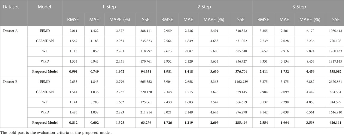
TABLE 5. Forecasting performance results of each model in Experiment 2.

For dataset A, in the 1-step to 3-step wind power forecasting, the CEEMDAN-WT secondary decomposition technique combined forecasting model proposed has the best forecasting effect. In the 1-step forecasting, the MAPE values of EEMD, CEEMDAN, WPD and WT were 3.527%, 2.933%, 2.283% and 2.431%, respectively. It can be seen that the forecasting effect of WT was better in the 1-step forecasting. In the 2-step and 3-step forecasting, CEEMDAN combined forecasting had better forecasting performance, and its 2-step and 3-step MAPE values were 4.653% and 5.236%, respectively.

For dataset B, according to the four evaluation criteria, it can be concluded that the proposed combined forecasting model of CEEMDAN-WT secondary decomposition technique still has the best prediction effect among 1-step to 3-step forecasting, and the MAPE values of 1-step, 2-step and 3-step are 1.325%%, 2.693% and 3.538% respectively. In addition, in 1-step and 2-step forecast, WT combined forecasting has better prediction effect, and its MAPE value was 1.662% and 3.542%, respectively; in 3-step forecasting, CEEMDAN combined forecast has better prediction accuracy, and its corresponding MAPE value is 4.442%.

4.4.2.1 Remark

According to the evaluation criteria in experiment 2, it was obvious that for all dataset and forecasting steps, the combined forecasting model of CEEMDAN-WT secondary decomposition technique had the smallest RMSE, MAE and MAPE values. Therefore, it can be concluded that the forecasting performance of CEEMDAN-WT secondary decomposition technique combined forecasting model is better than other data decomposition combined forecasting models.

4.4.3 Experiment 3

Experiment 3 includes four forecasting models, including CEEMDAN-GWO-LSSVM, CEEMDAN-GWO-ELM, CEEMDAN-GWO-BPNN, and Proposed Model. Figure 11 is the chart of the forecasting error of dataset A and dataset B in experiment 3, and Table 6 shows the comparison of the evaluation criteria results of experiment 3.

FIGURE 11

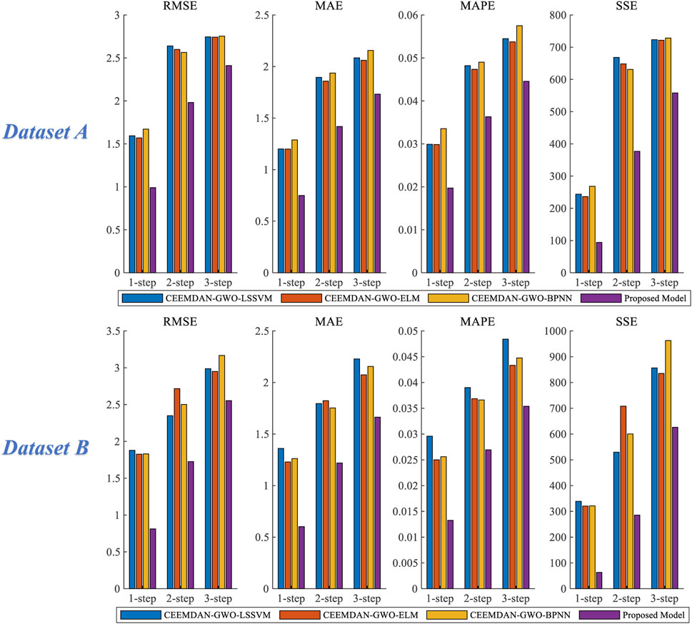
FIGURE 11. Comparison of the evaluation criteria of each model of Experiment 3.

TABLE 6

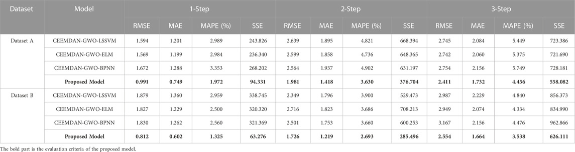
TABLE 6. Forecasting performance results of each model in Experiment 3.

For dataset A, in the 1-step forecast, the RMSE, MAE, MAPE and SSE of the proposed model are 0.991, 0.749, 1.972% and 94.331 respectively. The MAPE of the four forecasting models are Proposed Model, CEEMDAN-GWO-ELM, CEEMDAN-GWO-LSSVM and CEEMDAN-GWO-BPNN from low to high, and the MAPE values are 1.972%, 2.984%, 2.989% and 3.353%, respectively. The MAPE values of proposed model in 2-step and 3-step forecasts are 3.630% and 4.456%, respectively. It can be seen that the prediction accuracy of proposed model is the highest among the 1-step, 2-step and 3-step forecasts.

For dataset B, the MAPE values of proposed model are 1.325%, 2.693% and 3.538% in 1-step, 2-step and 3-step predictions, respectively. In the 3-step forecasting, the MAPE value of the proposed model is 1.302%, 1.796% and 0.938% lower than that of CEEMDAN-GWO-LSSVM, CEEMDAN-GWO-ELM and CEEMDAN-GWO-BPNN respectively. The prediction accuracy of proposed model is still better than the other three models.

4.4.3.1 Remark

As can be seen from the results of 1-step, 2-step and 3-step forecasting obtained in Experiment 3, the evaluation criteria of the proposed combined prediction model based on CEEMDAN and WT secondary decomposition is significantly lower than that based on CEEMDAN decomposition.

4.4.4 Experiment 4

Experiment 4 includes several classic machine learning prediction models, including LSSVM, ELM, BPNN, WNN, DBN and Proposed Model. Figure 12 shows the bar chart of prediction error of dataset A and dataset B in experiment 4, and Table 7 shows the comparison of the evaluation index results of experiment 4.

FIGURE 12

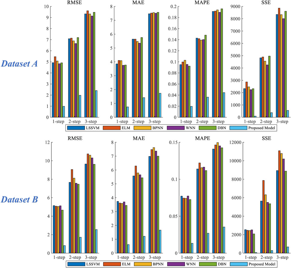
FIGURE 12. Comparison of the evaluation criteria of each model of Experiment 4.

TABLE 7

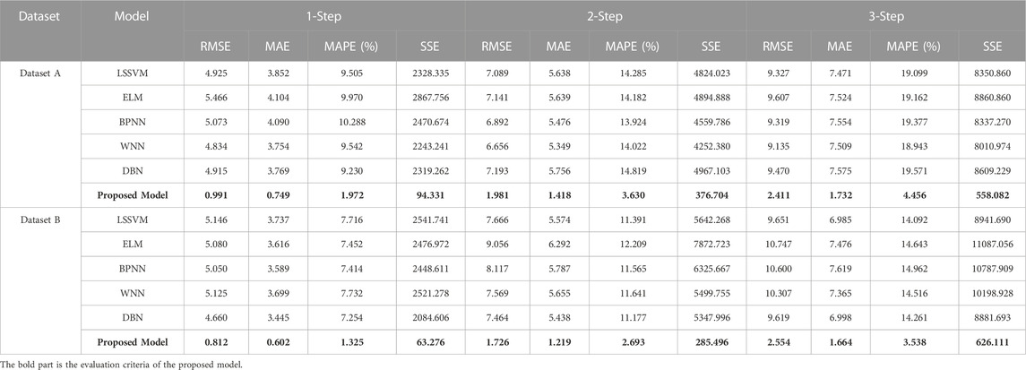
TABLE 7. Forecasting performance results of each model in Experiment 4.

For dataset A, in all the forecasting steps, the evaluation criteria of proposed model are significantly lower than that of other forecasting models. In the 3-step forecasting, the MAPE values of LSSVM, ELM, BPNN, WNN and DBN are 19.099%, 19.162%, 19.377%, 18.943% and 19.571%, respectively. In comparison, the MAPE value of the Proposed Model is 4.456%, which is reduced by 14.643%, 14.706%, 14.921%, 14.487% and 15.115%, respectively.

For Dataset B, in all the prediction steps, based on the four evaluation criteria used, Proposed Model is still significantly better than other prediction models. The MAPE values of 1-step, 2-step and 3-step are 1.325%, 2.693% and 3.538%, respectively, which has the smallest error compared with other prediction models. Taking the three-step prediction result as an example, the map value of The Proposed model decreased by 10.554%, 11.105%, 11.424%, 10.978% and 10.723%, respectively, compared with LSSVM, ELM, BPNN, WNN and DBN forecasting model.

4.4.4.1 Remark

In Experiment 4, the forecasting results of proposed model and other three forecasting models are significantly different. It can be seen that the combined forecasting model based on secondary decomposition has better wind power forecasting effect than the traditional single forecasting model.

5 Conclusion

Short-term wind power forecasting is of great significance to the operation of power system. However, the intermittence, randomness and high volatility of wind power limit the development of wind power. Therefore, it is very necessary to develop an accurate wind power forecasting model. In this study, a combined forecasting model based on secondary decomposition data processing technology and parameter optimization is proposed. Compared with other prediction models, the main contributions of this model are as follows: 1) Three individual prediction models are established, which are SDT-GWO-LSSVM,SDT-GWO-ELM and SDT-GWO-BPNN respectively. The combination forecasting model is established by using GWO algorithm to determine the optimal weight coefficient. In experiment 1, the three single forecasting models are compared with the proposed combination forecasting model, and the results show that the prediction accuracy of the proposed combination forecasting model is better than that of the single forecasting model. 2) Comparing experiment 1 with experiment 3, the prediction accuracy of SDT-GWO-LSSVM,SDT-GWO-ELM and SDT-GWO-BPNN prediction model based on secondary decomposition is improved compared with CEEMDAN-GWO-LSSVM,CEEMDAN-GWO-ELM and CEEMDAN-GWO-BPNN prediction model of single decomposition. It is verified that the use of CEEMDAN and WT secondary decomposition technology to preprocess wind power data reduces the difficulty of prediction, is conducive to better extraction of the characteristics of wind power series, and has a better prediction effect than the traditional single decomposition technology. 3) In experiment 2, the combination forecasting models of other data decomposition methods are compared, and the combination forecasting model based on secondary decomposition proposed in this paper has better prediction performance in data set An and data set B. this shows that the CEEMDAN-WT secondary decomposition strategy is better than other decomposition methods. 4) In experiment 4, the combination forecasting model is compared with several classical prediction models, from the point of view of evaluation criteria, the combination forecasting model is obviously better than other prediction models. Through the analysis of the results of experiment 1, experiment 2, experiment 3 and experiment 4, the prediction error of the proposed combination forecasting model is the smallest. Therefore, the proposed combination model has a broad application prospect in short-term wind power forecasting.

The next research work can be carried out from the following aspects: 1) Adopt relevant strategies to improve the GWO to enhance the optimization ability of the algorithm and improve the prediction performance of the model. 2) More single forecasting models are established to expand the model base, and the artificial intelligence method is adopted to select the optimal single forecasting model to construct the combined forecasting model to enhance the robustness of the combined forecasting model. 3) Adopt a more efficient strategy to select the optimal weight coefficient of the combination forecasting model.

Data availability statement

The raw data supporting the conclusions of this article will be made available by the authors, without undue reservation.

Author contributions

ZS: experiments, data processing, writing original draft. BZ: Manuscript modification, Data visualization. HL: supervision, project administration, review. All authors listed have made a substantial, direct, and intellectual contribution to the work and approved it for publication.

Funding

This work is supported by Open Research Fund of Wanjiang Collaborative Innovation Center for High-end Manufacturing Equipment, Award Number: GCKJ2018013; Research Project of Anhui Polytechnic University, Award Number: Xjky2020022; Graduate Education Innovation Fund of Anhui Polytechnic University.

Conflict of interest

The authors declare that the research was conducted in the absence of any commercial or financial relationships that could be construed as a potential conflict of interest.

Publisher’s note

All claims expressed in this article are solely those of the authors and do not necessarily represent those of their affiliated organizations, or those of the publisher, the editors and the reviewers. Any product that may be evaluated in this article, or claim that may be made by its manufacturer, is not guaranteed or endorsed by the publisher.

References

Bahrami, S., Hooshmand, R., and Parastegari, M. (2014). Short term electric load forecasting by wavelet transform and grey model improved by PSO (particle swarm optimization) algorithm. Energy 72, 434–442. doi:10.1016/j.energy.2014.05.065

CrossRef Full Text | Google Scholar

Bento, P. M. R., Pombo, J. A. N., Calado, M. R. A., and Mariano, S. J. P. S. (2019). Optimization of neural network with wavelet transform and improved data selection using bat algorithm for short-term load forecasting. Neurocomputing 358, 53–71. doi:10.1016/j.neucom.2019.05.030

CrossRef Full Text | Google Scholar

Chen, G., Tang, B., Zeng, X., Zhou, P., Kang, P., and Long, H. Y. (2022). Short-term wind speed forecasting based on long short-term memory and improved BP neural network. Int. J. Electr. Power & Energy Syst. 134, 107365. doi:10.1016/j.ijepes.2021.107365

CrossRef Full Text | Google Scholar

Chen, H., Birkelund, Y., Batalden, B., and Barabadi, A. (2022). Noise-intensification data augmented machine learning for day-ahead wind power forecast. Energy Rep. 8, 916–922. doi:10.1016/j.egyr.2022.05.265

CrossRef Full Text | Google Scholar

Ding, J., Chen, G., Huang, Y., Zhu, Z., Yuan, K., and Xu, H. (2021). Short-term wind speed prediction based on CEEMDAN-SE-improved PIO-GRNN model. Meas. Control 54 (1-2), 73–87. doi:10.1177/0020294020981400

CrossRef Full Text | Google Scholar

Dong, L., Yuan, X. F., Yan, B. S., Song, Y., Xu, Q. Y., and Yang, X. Y. (2022). An improved grey wolf optimization with multi-strategy ensemble for robot path planning. Sensors-Basel 22 (18), 6843. doi:10.3390/s22186843

PubMed Abstract | CrossRef Full Text | Google Scholar

Du, P., Wang, J., Guo, Z., and Yang, W. (2017). Research and application of a novel hybrid forecasting system based on multi-objective optimization for wind speed forecasting. Energy. Convers. manage. 150, 90–107. doi:10.1016/j.enconman.2017.07.065

CrossRef Full Text | Google Scholar

Duan, J., Wang, P., Ma, W., Fang, S., and Hou, Z. (2022). A novel hybrid model based on nonlinear weighted combination for short-term wind pow-er forecasting. Int. J. Electri-cal Power & Energy Syst. 134, 107452. doi:10.1016/j.ijepes.2021.107452

CrossRef Full Text | Google Scholar

Elia Transmission Company (2021). Wind power generation data. [Online]. Available: https://www.elia.be/en/grid-data/power-generation/wind-power-generation.

Google Scholar

Erdem, E., and Shi, J. (2011). ARMA based approaches for forecasting the tuple of wind speed and direction. Apply. Energy 88 (4), 1405–1414. doi:10.1016/j.apenergy.2010.10.031

CrossRef Full Text | Google Scholar

Hu, J., Wang, J., Zeng, G., and Zeng, G. (2013). A hybrid forecasting approach applied to wind speed time series. Renew. Energy 60, 185–194. doi:10.1016/j.renene.2013.05.012

CrossRef Full Text | Google Scholar

Hu, S., Xiang, Y., Huo, D., Jawad, S., and Liu, J. (2021). An improved deep belief network based hybrid forecasting method for wind power. Energy 224, 120185. doi:10.1016/j.energy.2021.120185

CrossRef Full Text | Google Scholar

Hu, W., Yang, Q., Chen, H. P., Yuan, Z., Li, C., Shao, S., et al. (2021). New hybrid approach for short-term wind speed predictions based on preprocessing algorithm and optimization theory. Renew. Energy. 179, 2174–2186. doi:10.1016/j.renene.2021.08.044

CrossRef Full Text | Google Scholar

Hua, L., Zhang, C., Peng, T., Ji, C., and Shahzad Nazir, M. (2022). Integrated framework of extreme learning machine (ELM) based on improved atom search optimization for short-term wind speed prediction. Energy. Convers. manage. 252, 115102. doi:10.1016/j.enconman.2021.115102

CrossRef Full Text | Google Scholar

Huang, G., Zhu, Q., and Siew, C. (2006). Extreme learning machine: Theory and applications. Neurocomputing 70 (1), 489–501. doi:10.1016/j.neucom.2005.12.126

CrossRef Full Text | Google Scholar

Huang, Z., and Chalabi, Z. S. (1995). Use of time-series analysis to model and forecast wind speed. J. Wind Eng. Industrial Aerodynamics 56 (2), 311–322. doi:10.1016/0167-6105(94)00093-s

CrossRef Full Text | Google Scholar

Jalali, S., Ahmadian, S., Khodayar, M., Khosravi, A., Shafie-khah, M., Nahavandi, S., et al. (2022). An advanced short-term wind power forecasting framework based on the optimized deep neural network models. Int. J. Electr. POWER & ENERGY Syst. 141, 108143. doi:10.1016/j.ijepes.2022.108143

CrossRef Full Text | Google Scholar

Khazaei, S., Ehsan, M., Soleymani, S., and Mohammadnezhad-Shourkaei, H. (2022). A high-accuracy hybrid method for short-term wind power forecasting. Energy 238, 122020. doi:10.1016/j.energy.2021.122020

CrossRef Full Text | Google Scholar

Li, L., Zhao, X., Tseng, M., and Tan, R. R. (2020). Short-term wind power forecasting based on support vector machine with improved dragonfly algorithm. J. Clean. Prod. 242, 118447. doi:10.1016/j.jclepro.2019.118447

CrossRef Full Text | Google Scholar

Liao, C., Wang, I., Lin, K., and Lin, Y. (2021). A fuzzy seasonal long short-term memory network for wind power forecasting. Mathematics 9 (11), 1178. doi:10.3390/math9111178

CrossRef Full Text | Google Scholar

Lin, B., and Zhang, C. (2021). A novel hybrid machine learning model for short-term wind speed prediction in inner Mongolia, China. Renew. Energy. 179, 1565–1577. doi:10.1016/j.renene.2021.07.126

CrossRef Full Text | Google Scholar

Liu, D., Niu, D., Wang, H., and Fan, L. (2014). Short-term wind speed forecasting using wavelet transform and support vector machines optimized by genetic algorithm. Renew. Energy 62, 592–597. doi:10.1016/j.renene.2013.08.011

CrossRef Full Text | Google Scholar

Lu, P., Ye, L., Zhong, W., Qu, Y., Zhai, B., Tang, Y., et al. (2020). A novel spatio-temporal wind power forecasting framework based on multi-output support vector machine and optimization strategy. J. Clean. Prod. 254, 119993. doi:10.1016/j.jclepro.2020.119993

CrossRef Full Text | Google Scholar

Meng, A., Chen, S., Ou, Z., Ding, W., Zhou, H., Fan, J., et al. (2022). A hybrid deep learning architecture for wind power prediction based on bi-attention mechanism and crisscross optimization. Energy 238, 121795. doi:10.1016/j.energy.2021.121795

CrossRef Full Text | Google Scholar

Mirjalili, S., Mirjalili, S. M., and Lewis, A. (2014). Grey wolf optimizer. Adv. Eng. Softw. 69, 46–61. doi:10.1016/j.advengsoft.2013.12.007

CrossRef Full Text | Google Scholar

Nguyen, T., and Phan, Q. B. (2022). Hourly day ahead wind speed forecasting based on a hybrid model of EEMD, CNN-Bi-LSTM embedded with GA optimization. Energy Rep. 8, 53–60. doi:10.1016/j.egyr.2022.05.110

CrossRef Full Text | Google Scholar

Ogliari, E., Guilizzoni, M., Giglio, A., and Pretto, S. (2021). Wind power 24-h ahead forecast by an artificial neural network and an hybrid model: Comparison of the predictive performance. Renew. Energy. 178, 1466–1474. doi:10.1016/j.renene.2021.06.108

CrossRef Full Text | Google Scholar

Peng, T., Zhou, J., Zhang, C., and Zheng, Y. (2017). Multi-step ahead wind speed forecasting using a hybrid model based on two-stage decomposition technique and AdaBoost-extreme learning machine. Energy. Convers. Manage 153, 589–602. doi:10.1016/j.enconman.2017.10.021

CrossRef Full Text | Google Scholar

Rajput, S. S., Bohat, V. K., and Arya, K. V. (2019). Grey wolf optimization algorithm for facial image super-resolution. Appl. Intell. 49 (4), 1324–1338. doi:10.1007/s10489-018-1340-x

CrossRef Full Text | Google Scholar

Rajput, S. S., and S-Gwo-Fh, (2022). S-GWO-FH: Sparsity-based grey wolf optimization algorithm for face hallucination. Soft Comput. 26 (18), 9323–9338. doi:10.1007/s00500-022-07250-1

CrossRef Full Text | Google Scholar

Ren, C., An, N., Wang, J., Li, L., Hu, B., and Shang, D. (2014). Optimal parameters selection for BP neural network based on particle swarm optimization: A case study of wind speed forecasting. Knowledge-Based Syst. 56, 226–239. doi:10.1016/j.knosys.2013.11.015

CrossRef Full Text | Google Scholar

Soman, S. S., Zareipour, H., Malik, O., and Mandal, P. (2010). A review of wind power and wind speed forecasting methods with different time horizons in Proceedings of the North american power symposium 2010, Arlington, TX, USA, 26-28 September 2010 (IEEE), 1–8.

Tascikaraoglu, A., and Uzunoglu, M. (2014). A review of combined approaches for prediction of short-term wind speed and power. Renew. Sustain. Energy Rev. 34, 243–254. doi:10.1016/j.rser.2014.03.033

CrossRef Full Text | Google Scholar

Wang, J., Zhang, L., Wang, C., and Liu, Z. (2021). A regional pretraining-classification-selection forecasting system for wind power point forecasting and interval forecasting. Appl. Soft Comput. 113, 107941. doi:10.1016/j.asoc.2021.107941

CrossRef Full Text | Google Scholar

Wang, Y. T., Li, C. H., and Yang, K. (2020). Coordinated control and dynamic optimal dispatch of islanded microgrid system based on GWO. Symmetry-Basel 12 (8), 1366. doi:10.3390/sym12081366

CrossRef Full Text | Google Scholar

Xiang, L., Deng, Z., and Hu, A. (2019). Forecasting short-term wind speed based on IEWT-LSSVM model optimized by bird swarm algorithm. IEEE Access 7, 59333–59345. doi:10.1109/access.2019.2914251

CrossRef Full Text | Google Scholar

Xiao, L., Wang, J., Dong, Y., and Wu, J. (2015). Combined forecasting models for wind energy forecasting: A case study in China. Renew. Sustain. Energy Rev. 44, 271–288. doi:10.1016/j.rser.2014.12.012

CrossRef Full Text | Google Scholar

Xiong, B., Lou, L., Meng, X., Wang, X., Ma, H., and Wang, Z. (2022). Short-term wind power forecasting based on attention mechanism and deep learning. Electr. Power Syst. Res. 206, 107776. doi:10.1016/j.epsr.2022.107776

CrossRef Full Text | Google Scholar

Yin, H., Ou, Z., Fu, J., Cai, Y., Chen, S., and Meng, A. (2021). A novel transfer learning approach for wind power prediction based on a serio-parallel deep learning architecture. Energy 234, 121271. doi:10.1016/j.energy.2021.121271

CrossRef Full Text | Google Scholar

Zhang, C. C., Liu, Y. F., and Hu, C. H. (2022). Path planning with time windows for multiple UAVs based on gray wolf algorithm. BIOMIMETICS 7 (4), 225. doi:10.3390/biomimetics7040225

PubMed Abstract | CrossRef Full Text | Google Scholar

Zhang, K., Qu, Z., Wang, J., Zhang, W., and Yang, F. (2017). A novel hybrid approach based on cuckoo search optimization algorithm for short-term wind speed forecasting. Environ. Prog. Sustain. Energy 36 (3), 943–952. doi:10.1002/ep.12533

CrossRef Full Text | Google Scholar

Zhang, P., Li, C., Peng, C., and Tian, J. (2020). Ultra-short-term prediction of wind power based on error following forget gate-based long short-term memory. Energies 13 (20), 5400. doi:10.3390/en13205400

CrossRef Full Text | Google Scholar

Zhang, Y., and Li, R. (2022). Short term wind energy prediction model based on data decomposition and optimized LSSVM. Sustain. Energy Technol. Assessments 52, 102025. doi:10.1016/j.seta.2022.102025

CrossRef Full Text | Google Scholar

Zhang, Z., Qin, H., Liu, Y., Yao, L., Yu, X., Lu, J., et al. (2019). Wind speed forecasting based on quantile regression minimal gated memory network and kernel density estimation. Energy. Convers. manage. 196, 1395–1409. doi:10.1016/j.enconman.2019.06.024

CrossRef Full Text | Google Scholar

Zhou, Y., Wang, J., Lu, H., and Zhao, W. (2022). Short-term wind power prediction optimized by multi-objective dragonfly algorithm based on variational mode decomposition,” Chaos. Solit. Fractals 157, 111982. doi:10.1016/j.chaos.2022.111982

CrossRef Full Text | Google Scholar

Zhu, T., Wang, W. B., and Yu, M. (2022). Short-term wind speed prediction based on FEEMD-PE-SSA-BP. Environ. Environ. Sci. Pollut. Res. 29, 79288–79305. doi:10.1007/s11356-022-21414-4

PubMed Abstract | CrossRef Full Text | Google Scholar