Multi-time scale stochastic production simulation under VHVDC long-term contract trading electricity quantity constraint

A two-layer multi-time scale stochastic production simulation framework is constructed to account for the long-term contract electricity quantity of ultra-high voltage direct current (UHVDC) transmission. On the upper layer, based on the characteristics of load demand and renewable energy output extracted from the historical operating data, monthly and daily production simulation models are carried out considering the seasonal characteristics of hydropower during a high-water period and low-water period to optimize the distribution of contract electric quantity sending through UHVDC transmission in the target year or month. According to the DC transmission electric quantity optimized by the daily production simulation in the upper layer, together with the forecast scenario, the lower layer of the framework provides the optimization of day-ahead scheduling and intra-day rolling dispatch in the implementation process. The day-ahead dispatch optimization makes full use of the adjustment capability of transmission and optimizes the DC transmission electric quantity correction. Its compensation is based on the result of the daily production simulation, then the correction will be returned to the upper layer to restart the optimization of the remaining UHVDC contract electric quantity of the subsequent period and its distribution plan. Combined with the day-ahead DC transmission plan, the intra-day rolling optimization is carried out to adjust the output of the unit using more accurate forecasting scenarios. The distributionally robust optimization model is used in the lower layer to convert an uncertain problem into a deterministic quadratically constrained quadratic programming (QCQP) problem according to the form of an uncertain distribution set. Then the QCQP problem is further converted into a linear programming (LP) problem by using the reformulation linearization technique (RLT). A test system with the energy composition and distribution referring to a real provincial power grid in northwest China is established for verification. The results show that the proposed method can effectively improve the economics of system operation and the accommodation of renewable energy based on ensuring security.

1 Introduction

The dual-carbon goal will promote the rapid development of renewable energy in China. It is estimated that the total installed capacity of wind power and solar power will reach more than 1.2 billion kilowatts by 2030 (Xi, 2020). Due to the reverse distribution of load and installed capacity of renewable energy, the limited level of grid interconnection and other reasons, the difficulty of renewable energy consumption in some areas has become increasingly apparent (Shu et al., 2017). Transmission of surplus power across regions is an effective way to solve the above problems, and UHVDC transmission plays an important role in the long-distance cross-regional consumption of wind and solar resources (Liu et al., 2014). Usually, the transmission mode for UHVDC is established with a fixed power adjustment according to the regional long-term contract trading electric quantity (Zhong et al., 2015), which is difficult to give full play to the power regulation potential of DC transmission and cannot adapt to the massive random power output of renewable energy. It causes the abandonment of renewable energy and the increase of the peak-shaving pressure of traditional units.

The existing studies involving DC transmission plan mostly focus on optimizing the day-ahead or intra-day power distribution of the known daily DC transmission electric quantity (Li et al., 2021; Cui et al., 2022; Zhang et al., 2022). However, there is limited research on how to obtain the daily delivery of electric quantity from the long-time-scale DC electric quantity contract which is usually signed on a yearly or monthly basis. In addition, due to the uncertainty of the actual operation scenarios, it is also necessary to continuously update the subsequent remaining contract electric quantity and its distribution plan based on the actual power delivered every day.

In recent years, scholars have focused intensively on unit commitment and economic dispatch for the power grid with increasing stochastic power source permeability, and successively put forward the scenario method (Wang et al., 2008; Papavasiliou and Oren, 2011; Hao et al., 2020), chance-constrained programming (Wu et al., 2014; Wang et al., 2019; Xu et al., 2020) and robust optimization (Wei et al., 2016; Lu et al., 2020; Velloso et al., 2020). Among them, the probability of stochastic renewable energy output distribution of scenario method and chance-constrained programming is difficult to obtain accurately, which makes the optimization results have safety risks. Moreover, the result of robust optimization is conservative. To solve the above-mentioned contradictions, some researches combine chance-constrained programming and robust optimization and establish the distributionally robust optimization (DRO) method (Delage et al., 2010; Bian et al., 2015; Lubin et al., 2016; Wang et al., 2017; Zhang et al., 2017; Xie et al., 2018; Zhang et al., 2018; Zhou et al., 2018). According to the different probability distribution sets (ambiguity sets) introduced to describe the random variable, DRO has corresponding decision models and processing methods (Delage et al., 2010). proposes DRO under the constraints of first and second moments, in which, the distribution type in the set and the moment information are not fixed, and the correlation between the uncertainties is considered. Based on this (Zhou et al., 2018), proposes a new model equivalent transformation method by using this distribution set, and equivalently transforms the original problem into a QCQP problem, and uses the RLT relaxation model to optimize the real-time dispatch of the system with wind power and thermal power units. The conventional units involved in the study of power grid economic dispatch are mostly thermal power units, with few related to hydropower and other units (Shao et al., 2020). There are many hydropower and wind power generation resources in Northwest China, while its regional load is generally small. Much of the clean energy power generation is sent out through inter-provincial DC transmission lines. Therefore, it is especially necessary to consider the seasonal characteristics and reservoir capacity constraints of hydropower plants in the production simulation.

In view of the above problems, a two-layer framework of multi-time scale stochastic production simulation under VHVDC long-term contract trading electricity quantity constraint is established in this paper. According to the energy composition and distribution of a provincial power grid in northwest China, a test system is established to verify the effectiveness of the proposed framework and method.

2 Multi-time scale stochastic production simulation framework

In this paper, a two-layer framework of multi-time scale stochastic production simulation for the power grid at the sending-end with high-proportion renewable energy is established under the constraint of UHVDC long-term contract trading electric quantity. Based on the characteristics of the load and renewable energy output extracted from the historical operation data for many years, the electric quantity distribution of UHVDC transmission in each month and each day is optimized. During the actual implementation process, the hourly and 15-min scale delivery power through UHVDC and unit output are optimized according to the forecast information of load and renewable energy, and if necessary, the subsequent electric quantity distribution of UHVDC transmission will be updated. The framework considers the completeness and accuracy of the information at different time scales, from comprehensive, low-precision, large-scale overall power quantity planning to local, high-precision, small-scale scheduling optimization, thus improving the reliability of optimization. The stochastic production simulation framework is shown in Figure 1.

1) The upper layer

FIGURE 1

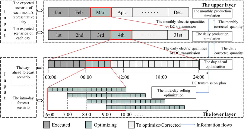
FIGURE 1. A two-layer framework for multi-time scale stochastic production simulation.

Through monthly and daily production simulation, together with the iteration between them, the upper layer of the framework can obtain the sending electric quantity of each month (or each day) through UHVDC transmission in the target year (or month) to be optimized. According to the expected scenario of the representative day of each month, the monthly production simulation optimizes the monthly distribution of electric quantity through UHVDC transmission under the contract trading electric quantity constraint of the target year. From this, the daily production simulation optimizes the daily electric quantity distribution in the target month according to the expected scenarios of each day in the target month to be optimized. The representative days and their expected scenarios of the target month for monthly production simulation and the expected scenario of each day in the target month for daily production simulation are both obtained by historical load demand and renewable energy output data mining. When the distribution result cannot meet the system operation constraints of a certain month, the fixed DC transmission electric quantity allocated to this month is taken as the constraint and optimize the daily DC transmission electric quantity in this month, and return the sum of the daily electric quantities to the monthly production simulation as the electric quantity correction of this month, then restart the monthly production simulation for the optimization of unexecuted months. The long-term production simulation can not only determine the distribution of DC transmission electric quantity in the following year by year-ahead optimization but also determine the DC transmission electric quantity in each unexecuted month or day by intra-year optimization combined with the correction information of the lower layer.

2) The lower layer

The lower layer of the framework optimizes the UHVDC transmission power and unit output power of the following period according to its DC transmission electric quantity plan optimized by the daily production simulation in the upper layer. The day-ahead dispatch can compensate for the DC transmission electric quantity given by the daily production simulation, and the electric quantity correction is sent back to the daily production simulation. The intra-day rolling dispatch optimizes the unit output power combined with more accurate short-time forecast information.

3) Iterative optimization of the upper and lower layers

The daily DC transmission electric quantities produced by the upper layer base on the expected scenarios may not completely suitable for the forecast scenarios in the economic scheduling of the lower layer. Therefore, these daily DC transmission electric quantities can be adjusted with compensation in the day-ahead optimization of the lower layer when necessary, and then the electric quantity correction is sent back to the daily production simulation and restart the daily production simulation to update the daily electric quantities for the remaining days of this month. When the iteration of this month is over, the corrected electric quantity of UHVDC transmission of this month is returned to the monthly production simulation and the electric quantities for the remaining months of this year are redistributed until the annual plan is completed.

4) Treatment of renewable energy output uncertainty

Considering the limited forecast accuracy of medium and long-term renewable energy output, in the monthly and daily production simulation of the upper layer, the expected scenario calculated based on long-term historical data is used to reflect the uncertainty of the system, and the long-term stochastic production simulation is carried out under the expected scenarios. The accuracy of day-ahead and intra-day forecast scenarios is better, but there are still forecast errors, which brings hidden risks to system safe operation. Therefore, the ambiguity set (Delage and Ye et al., 2010) is selected in the lower layer to describe the output forecast error of renewable energy units. Based on this, aiming at minimizing the operation cost under the forecast scenarios, the short-term DRO is carried out under the constraints of random variables.

3 Long-term stochastic production simulation

3.1 Objective function

The objective of long-term stochastic production simulation is to minimize the overall operation costs under the expected scenarios.

$\min {\displaystyle \sum }_{t\in \mathbb{T}}\left[\left({\displaystyle \sum }_{i\in \mathbb{G}}C\left(P_{i,t}\right)+C_t^{\mathrm{e}\mathrm{m}\mathrm{i}\mathrm{s}}\right)+\left(\delta {\displaystyle \sum }_{k\in \mathbb{K}}{A}_k{Q}_{k,t}^{\mathrm{s}}+\rho P_{n,t}^{\mathrm{c}\mathrm{u}\mathrm{r}\mathrm{t}}-{\lambda }_t{P}_{\mathrm{d}\mathrm{c},t}\right)\Delta t\right](1)$

$C\left(P_{i,t}\right)=\left({\alpha }_{i,1}{P}_{i,t}^2+{\alpha }_{i,2}{P}_{i,t}+{\alpha }_{i,3}\right)\Delta t(\mathrm{2a})$

$C_t^{\mathrm{e}\mathrm{m}\mathrm{i}\mathrm{s}}={\displaystyle \sum }_{i\in \mathbb{G}}{\upsilon }_i^{\mathrm{e}\mathrm{m}\mathrm{i}\mathrm{s}}{P}_{i,t}\Delta t(\mathrm{2b})$

where $\mathbb{T}$ is the set of time intervals in the calculation cycle; t is the serial number of time interval, the duration of each time interval is $\Delta t$; $\mathbb{G}$ is the set of thermal power units; i is the serial number of thermal power unit; $P_{i,t}$ is the output power of thermal power unit i in interval t; $C\left(P_{i,t}\right)$ is the power generation cost of thermal power unit i in interval t; $C_t^{\mathrm{e}\mathrm{m}\mathrm{i}\mathrm{s}}$ is the emission cost of system in interval t; δ is the electricity price of hydropower; $\mathbb{K}$ is the set of hydropower plants; k is the serial number of hydropower plant; $A_k$ is output coefficient of hydropower plant k; $Q_{k,t}^{\mathrm{s}}$ is the abandoned water spillage of hydropower plant k in interval t; ρ is the penalty factor of renewable energy power curtailment; $P_{n,t}^{\mathrm{c}\mathrm{u}\mathrm{r}\mathrm{t}}$ is the power curtailment of renewable energy unit n in interval t; λ_t is the price of DC transmission electric quantity in interval t; $P_{\mathrm{d}\mathrm{c},t}$ is the UHVDC transmission power in interval t; ${\alpha }_{i,1}$, ${\alpha }_{i,2}$ and ${\alpha }_{i,3}$ are the cost coefficients of thermal power unit i; ${\upsilon }_i^{\mathrm{e}\mathrm{m}\mathrm{i}\mathrm{s}}$ is the emission cost coefficients of thermal power unit i.

The specific process of the upper layer of the framework is shown in Supplementary Material S1.

3.2 Constraints

3.2.1 System operation constraint

System operation constraints include power balance constraint, branch transmission power constraint and system reserve capacity constraint, see (A1)-(A4) in Supplementary Material S2 for details.

3.2.2 Thermal power generation constraint

Thermal power generation constraints include the generator output power and the ramping up/down constraints, see (A5)-(A6) in Supplementary Material S3 for details.

3.2.3 Hydropower generation constraint

Hydropower generation needs to satisfy the constraints of unit output power, water consumption of power generation, reservoir capacity, water flow of power generation, abandoned water spillage, and water flow balance, see (A7)-(A12) in Supplementary Material S4 for details.

3.2.4 Renewable energy generation constraint

$\left(1-\varpi \right)P_{n,t}^{\mathrm{t}\mathrm{h}\mathrm{e}\mathrm{o}}\le P_{n,t}\le P_{n,t}^{\mathrm{t}\mathrm{h}\mathrm{e}\mathrm{o}}(3)$

where $P_{n,t}^{\mathrm{t}\mathrm{h}\mathrm{e}\mathrm{o}}$ is the theoretical output power for renewable energy unit n in interval t; $\varpi$ is the rate of renewable electric power curtailment.

3.2.5 UHVDC transmission constraint

1) DC transmission power constraint

${\underset{\_}{P}}_{\mathrm{d}\mathrm{c},t}\le P_{\mathrm{d}\mathrm{c},t}\le \min \left\{{\overline{P}}_{\mathrm{L},t}^{\mathrm{r}\mathrm{e}\mathrm{c}},{\overline{P}}_{\mathrm{d}\mathrm{c},t}\right\}(4)$

2) The ramp rate of DC transmission power

$\left\{\begin{array}{l}{y}_t=1,\hspace{1em}{R}_{\mathrm{d}\mathrm{c}}^{\mathrm{d}\mathrm{n}}\le \left|P_{\mathrm{d}\mathrm{c},t}-P_{\mathrm{d}\mathrm{c},t-1}\right|\le R_{\mathrm{d}\mathrm{c}}^{\mathrm{u}\mathrm{p}}\\ y_t=0,\hspace{1em}\left|P_{\mathrm{d}\mathrm{c},t}-P_{\mathrm{d}\mathrm{c},t-1}\right|=0\end{array}\right.(5)$

3) Regulation times constraint of UHVDC transmission during a day

${\displaystyle \sum }_{t=1}^T{y}_t\le \overline{\mathrm{\Psi }}(6)$

where ${\overline{P}}_{\mathrm{d}\mathrm{c},t}$ and ${\underset{\_}{P}}_{\mathrm{d}\mathrm{c},t}$ are the upper and lower limits of DC transmission power; ${\overline{P}}_{\mathrm{L},t}^{\mathrm{r}\mathrm{e}\mathrm{c}}$ is the maximum receivable power of the receiving-end power grid; y_t is the adjustment status variable, “1” means that the DC transmission power in interval t has been adjusted compared with that in interval t-1, “0” means unadjusted; $R_{\mathrm{d}\mathrm{c}}^{\mathrm{u}\mathrm{p}}$ and $R_{\mathrm{d}\mathrm{c}}^{\mathrm{d}\mathrm{n}}$ are the ramp-up and ramp-down limits of DC transmission power for each time respectively; T is the total number of time intervals in a day; $\overline{\mathrm{\Psi }}$ is the upper limit of adjustment times for DC transmission power in a day. In order to maintain the stability of UHVDC, the DC transmission power should be kept constant for a period of time after each adjustment.

4) Constraint of trading electric quantity

$\underset{\_}{E}-f_{\mathbb{M}}\left(P_{\mathrm{d}\mathrm{c},m,t},\Delta E_m\right)\le E^{\mathrm{r}\mathrm{e}\mathrm{s}}\le \overline{E}-f_{\mathbb{M}}\left(P_{\mathrm{d}\mathrm{c},m,t},\Delta E_m\right)(\mathrm{7a})$

$f_{\mathbb{M}}\left(P_{\mathrm{d}\mathrm{c},m,t},\Delta E_m\right)={\displaystyle \sum }_{m\in \mathbb{M}}\left({\zeta }_m{\displaystyle \sum }_{t\in T_{\mathrm{a}}}{P}_{\mathrm{d}\mathrm{c},m,t}\Delta t+\Delta E_m\right)(\mathrm{7b})$

${\underset{\_}{E}}_m-f_{\mathbb{D}}\left(P_{\mathrm{d}\mathrm{c},d,t},\Delta E_d\right)\le E_m^{\mathrm{r}\mathrm{e}\mathrm{s}}\le {\overline{E}}_m-f_{\mathbb{D}}\left(P_{\mathrm{d}\mathrm{c},d,t},\Delta E_d\right)(\mathrm{8a})$

$f_{\mathbb{D}}\left(P_{\mathrm{d}\mathrm{c},d,t},\Delta E_d\right)={\displaystyle \sum }_{d\in \mathbb{D}}\left({\displaystyle \sum }_{t\in T_{\mathrm{a}}}{P}_{\mathrm{d}\mathrm{c},d,t}\Delta t+\Delta E_d\right)(\mathrm{8b})$

where $\overline{E}$ and $\underset{\_}{E}$ are the upper and lower limits of DC transmission contract electric quantity of a year; ${\overline{E}}_m$ and ${\underset{\_}{E}}_m$ are the upper and lower limits of DC transmission contract electric quantity of month m; $\mathbb{M}$ and $\mathbb{D}$ are the sets of executed months and executed days respectively; $f_{\mathbb{M}}\left(P_{\mathrm{d}\mathrm{c},m,t},\Delta E_m\right)$ and $f_{\mathbb{D}}\left(P_{\mathrm{d}\mathrm{c},d,t},\Delta E_d\right)$ are the DC transmission electric quantity of the executed months and the executed days in the current month respectively; $P_{\mathrm{d}\mathrm{c},m,t}$ and $P_{\mathrm{d}\mathrm{c},d,t}$ are the DC transmission power in interval t of month m and day d respectively; $\Delta E_m$ and $\Delta E_d$ are the corrected electric quantity of DC transmission of month m and day d respectively; $E^{\mathrm{r}\mathrm{e}\mathrm{s}}$ and $E_m^{\mathrm{r}\mathrm{e}\mathrm{s}}$ are the remaining electric quantity to be distributed in the current year and current month respectively; ${\zeta }_m$ is the maximum number of days in month m.

4 Short-term DRO

4.1 Unit failure risk cost model

Compared with the uncertainty of wind/load, the power system operation is more seriously affected by unit failure and outage (Zhang et al., 2019). In this paper, the uncertainty of renewable energy is mainly regulated by thermal power and hydropower units. Therefore, the failure risk cost model of thermal power units is established by referring to the reference (Shao et al., 2022).

Risk cost caused by thermal power unit failure:

$A\left(P_t^{\mathrm{b}\mathrm{a}\mathrm{s}\mathrm{e}}\right)={\mathrm{C}}_{\mathrm{L}}{E}_t^{\mathrm{U}}(9)$

where $A\left(P_t^{\mathrm{b}\mathrm{a}\mathrm{s}\mathrm{e}}\right)$ is the risk cost caused by thermal power unit failure; ${\mathrm{C}}_{\mathrm{L}}$ is the unit loss of load cost; $E_t^{\mathrm{U}}$ is the expected value of thermal power unit failure in interval t.

The probability of a single unit failure is:

$P{R}_{\mathrm{G},i,t}=P{R}_{i,t}\prod _{y\ne i}\left(1-P{R}_{y,t}\right)i,y\in \mathbb{G}(10)$

where $P{R}_{\mathrm{G},i,t}$ is the probability that only unit $i$ fails at time $t$; $P{R}_{i,t}$ is the probability that unit $i$ fails in interval t.; $\mathbb{G}$ is the set of all units.

The formula for calculating $E_t^{\mathrm{U}}$ is:

$E_t^{\mathrm{U}}={\displaystyle \sum }_{i\in \mathbb{G}}P{R}_{\mathrm{G},i,t}{P}_{i,t}^{\mathrm{b}\mathrm{a}\mathrm{s}\mathrm{e}}(11)$

where $P_{i,t}^{\mathrm{b}\mathrm{a}\mathrm{s}\mathrm{e}}$ is the base point for thermal power unit $i$ in interval t.

4.2 Objective function

The objective of short-term DRO is to minimize the overall operation costs of forecast scenarios.

$\min {\displaystyle \sum }_{t\in \mathbb{T}}\left[({\displaystyle \sum }_{i\in \mathbb{G}}C\left(P_{i,t}^{base}\right)+C_t^{emis})+(\delta {\displaystyle \sum }_{h\in \mathbb{H}}{A}_h{Q}_{h,t}^s-{\lambda }_t{P}_{dc,t}+\tau \Delta P_{dc,t}+\rho P_{n,t}^{curt})\Delta t+A\left(P_t^{\text{base}}\right)\right](12)$

where τ is the modified price for DC transmission electric quantity; $\Delta P_{\mathrm{d}\mathrm{c},t}$ is the corrected DC transmission power in interval t by day-ahead optimization.

The specific process of the DRO in the lower layer of the framework is shown in Supplementary Material S5.

4.3 Constraints and distribution set construction

4.3.1 Constraints

1) Power balance constraint

${\displaystyle \sum }_{i\in \mathbb{G}}{P}_{i,t}^{\mathrm{b}\mathrm{a}\mathrm{s}\mathrm{e}}+{\displaystyle \sum }_{j\in \mathbb{J}}{P}_{j,t}^{\mathrm{b}\mathrm{a}\mathrm{s}\mathrm{e}}+{\displaystyle \sum }_{n\in \mathbb{N}}{P}_{n,t}=P_{\mathrm{L},t}+P_{\mathrm{d}\mathrm{c},t}(13)$

$P_{n,t}=P_{n,t}^{\mathrm{t}\mathrm{h}\mathrm{e}\mathrm{o}}-P_{n,t}^{\mathrm{c}\mathrm{u}\mathrm{r}\mathrm{t}}(14)$

where $P_{j,t}^{\mathrm{b}\mathrm{a}\mathrm{s}\mathrm{e}}$ is the base point for hydropower unit j in interval t.

2) The constraints of adjustment factor

In this paper, a random variable vector ${\mathit{\Omega }}_t$ is established to represent the output power forecast error of each renewable energy unit. An adjustment factor is introduced to represent the power forecast error shared by each adjustable unit, then the output power of each adjustable unit is:

$P_{i,t}=P_{i,t}^{\mathrm{b}\mathrm{a}\mathrm{s}\mathrm{e}}-{\sigma }_{i,t}{\mathit{e}}^{\mathrm{T}}{\mathit{\Omega }}_t(\mathrm{15a})$

$P_{j,t}=P_{j,t}^{\mathrm{b}\mathrm{a}\mathrm{s}\mathrm{e}}-{\sigma }_{j,t}{\mathit{e}}^{\mathrm{T}}{\mathit{\Omega }}_t(\mathrm{15b})$

${\displaystyle \sum }_{i\in \mathbb{G}}{\sigma }_{i,t}+{\displaystyle \sum }_{j\in \mathbb{J}}{\sigma }_{j,t}=1,\hspace{1em}t\in \mathbb{T}(16)$

where e is the column vector with all elements being one; ${\sigma }_{i,t}$ is the adjustment factor of thermal power unit i in interval t; ${\sigma }_{j,t}$ is the adjustment factor of hydropower unit j in interval t.

3) Robust chance constraint

$\underset{{\mathit{\Omega }}_t\in \mathit{D}}{\inf }\mathrm{Pr}\left\{P_{i,t}^{\mathrm{b}\mathrm{a}\mathrm{s}\mathrm{e}}-{\sigma }_{i,t}{\mathit{e}}^{\mathrm{T}}{\mathit{\Omega }}_t\le {\overline{P}}_i\right\}\ge 1-\epsilon ,\hspace{1em}\forall i\in \mathbb{G}(\mathrm{17a})$

$\underset{{\mathit{\Omega }}_t\in \mathit{D}}{\inf }\mathrm{Pr}\left\{P_{i,t}^{\mathrm{b}\mathrm{a}\mathrm{s}\mathrm{e}}-{\sigma }_{i,t}{\mathit{e}}^{\mathrm{T}}{\mathit{\Omega }}_t\ge {\underset{\_}{P}}_i\right\}\ge 1-\epsilon ,\hspace{1em}\forall i\in \mathbb{G}(\mathrm{17b})$

$\underset{{\mathit{\Omega }}_t\in \mathit{D}}{\inf }\mathrm{Pr}\left\{P_{k,j,t}^{\mathrm{b}\mathrm{a}\mathrm{s}\mathrm{e}}-{\sigma }_{j,t}{\mathit{e}}^{\mathrm{T}}{\mathit{\Omega }}_t\le {\overline{P}}_{k,j}\right\}\ge 1-\epsilon ,\hspace{1em}\forall j\in \mathbb{J}(\mathrm{17c})$

$\underset{{\mathit{\Omega }}_t\in \mathit{D}}{\inf }\mathrm{Pr}\left\{P_{k,j,t}^{\mathrm{b}\mathrm{a}\mathrm{s}\mathrm{e}}-{\sigma }_{j,t}{\mathit{e}}^{\mathrm{T}}{\mathit{\Omega }}_t\ge {\underset{\_}{P}}_{\mathit{k,j}}\right\}\ge 1-\epsilon ,\hspace{1em}\forall j\in \mathbb{J}(\mathrm{17d})$

$\underset{{\mathit{\Omega }}_t\in \mathit{D}}{\inf }\mathrm{Pr}\left\{{\sigma }_{i,t}{\mathit{e}}^{\mathrm{T}}{\mathit{\Omega }}_t\le r_i^{\mathrm{u}\mathrm{p}}\right\}\ge 1-\epsilon ,\hspace{1em}\forall i\in \mathbb{G}(\mathrm{18a})$

$\underset{{\mathit{\Omega }}_t\in \mathit{D}}{\inf }\mathrm{Pr}\left\{{\sigma }_{i,t}{\mathit{e}}^{\mathrm{T}}{\mathit{\Omega }}_t\ge r_i^{\mathrm{d}\mathrm{n}}\right\}\ge 1-\epsilon ,\hspace{1em}\forall i\in \mathbb{G}(\mathrm{18b})$

$\underset{{\mathit{\Omega }}_t\in \mathit{D}}{\inf }\mathrm{Pr}\left\{{\sigma }_{j,t}{\mathit{e}}^{\mathrm{T}}{\mathit{\Omega }}_t\le r_j^{\mathrm{u}\mathrm{p}}\right\}\ge 1-\epsilon ,\hspace{1em}\forall j\in \mathbb{J}(\mathrm{18c})$

$\underset{{\mathit{\Omega }}_t\in \mathit{D}}{\inf }\mathrm{Pr}\left\{{\sigma }_{j,t}{\mathit{e}}^{\mathrm{T}}{\mathit{\Omega }}_t\ge r_j^{\mathrm{d}\mathrm{n}}\right\}\ge 1-\epsilon ,\hspace{1em}\forall j\in \mathbb{J}(\mathrm{18d})$

$P_{b,t}={\mathit{K}}_b^{\mathrm{G}\mathrm{T}}{\mathit{P}}_{\mathrm{G},t}+{\mathit{K}}_b^{\mathrm{J}\mathrm{T}}{\mathit{P}}_{\mathrm{J},t}+{\mathit{K}}_b^{\mathrm{N}\mathrm{T}}\left({\mathit{P}}_{\mathrm{N},t}+{\mathit{\Omega }}_t\right)-{\mathit{K}}_b^{\mathrm{L}\mathrm{T}}{\mathit{P}}_{\mathrm{L},t}-K_b^{\mathrm{d}\mathrm{c}}{P}_{\mathrm{d}\mathrm{c},t}(\mathrm{19a})$

$\underset{{\mathit{\Omega }}_t\in \mathit{D}}{\inf }\mathrm{Pr}\left\{\left|P_{b,t}\right|\le {\overline{P}}_b\right\}\ge 1-\epsilon ,\hspace{1em}\forall b\in \mathbb{B}(\mathrm{19b})$

where $1-\epsilon$ is the confidence level; $\mathit{D}$ is the distribution set that represents the uncertainty of ${\mathit{\Omega }}_t$, as shown in Eq. 17a; $r_i^{\mathrm{u}\mathrm{p}}$ and $r_i^{\mathrm{d}\mathrm{n}}$ are the upper and lower adjustment limits of thermal power unit i respectively; $r_j^{\mathrm{u}\mathrm{p}}$ and $r_j^{\mathrm{d}\mathrm{n}}$ are the upper and lower adjustment limits of hydropower unit j respectively. $P_{b,t}$ is the transmission power of line b in interval t; ${\mathit{K}}_b^{\mathrm{G}}$, ${\mathit{K}}_b^{\mathrm{J}}$ and ${\mathit{K}}_b^{\mathrm{N}}$ are the injection shift factor vectors of thermal power unit bus, hydropower unit bus and new energy unit bus to branch b respectively; Output vector for all thermal; ${\mathit{P}}_{\mathrm{G},t}$, ${\mathit{P}}_{\mathrm{J},t}$ and ${\mathit{P}}_{\mathrm{N},t}$ is the total output power vectors of all thermal power units, hydropower units and renewable energy units in interval t respectively.

4) Other constraints

The rest of the constraints are the same as Eqs 4–6, (A6) and (A8)-(A12).

4.3.2 Construction of distribution set

The ambiguity set D proposed in (Delage et al., 2010) is chosen to describe the uncertainty of ${\mathit{\Omega }}_t$ in this paper, which is as follows.

$\mathit{D}=\left\{\begin{array}{l}\int f\left({\mathit{\Omega }}_t\right)\mathrm{d}{\mathit{\Omega }}_t=1,\hspace{1em}f\left({\mathit{\Omega }}_t\right)\ge 0\\ {\left[E\left({\mathit{\Omega }}_t\right)-{\mathit{\mu }}_0\right]}^{\mathrm{T}}{\mathit{\Sigma }}_0^{-1}\left[E\left({\mathit{\Omega }}_t\right)-{\mathit{\mu }}_0\right]\le {\gamma }_1\\ E\left[\left({\mathit{\Omega }}_t-{\mathit{\mu }}_0\right){\left({\mathit{\Omega }}_t-{\mathit{\mu }}_0\right)}^{\mathrm{T}}\right]\preccurlyeq {\gamma }_2{\mathit{\Sigma }}_0\\ {\gamma }_1\ge 0,\hspace{1em}{\gamma }_2\ge 1\end{array}\right.(20)$

where $f\left({\mathit{\Omega }}_t\right)$ is the joint probability distribution function of ${\mathit{\Omega }}_t$; ${\mathit{\mu }}_0$, ${\mathit{\Sigma }}_0$ are statistical of the mean vector and statistical of the covariance matrix of ${\mathit{\Omega }}_t$ respectively; ${\gamma }_1$ and ${\gamma }_2$ are the conservative coefficients.

To sum up, Eqs 9–17 constitute the model of short-term DRO. However, it is difficult to solve the robust chance constraint directly, we need to transform it to an easy-to-solve model.

4.4 Conversion and solution.

4.1 Deterministic QCQP optimization problem

The key to solving the above short-term DRO model lies in the equivalent transformation of Eqs 14–16 (Zhang et al., 2022). gives an equivalent conversion method and proves it. Based on this method, the robust chance constraints of Eqs 14–16 can be transformed into Eqs 18–21, thus forming a deterministic QCQP optimization problem. The detailed transformation process is shown in Supplementary Material S6.

$-{\sigma }_{i,t}{\mathit{\mu }}_0^{\mathrm{T}}\mathit{e}+\xi {\sigma }_{i,t}\sqrt{{\mathit{e}}^{\mathrm{T}}{\mathit{\Sigma }}_0\mathit{e}}\le {\overline{P}}_i-P_{i,t}^{\mathrm{b}\mathrm{a}\mathrm{s}\mathrm{e}}(\mathrm{21a})$

${\sigma }_{i,t}{\mathit{\mu }}_0^{\mathrm{T}}\mathit{e}+\xi {\sigma }_{i,t}\sqrt{{\mathit{e}}^{\mathrm{T}}{\mathit{\Sigma }}_0\mathit{e}}\le P_{i,t}^{\mathrm{b}\mathrm{a}\mathrm{s}\mathrm{e}}-{\underset{\_}{P}}_i(\mathrm{21b})$

$-{\sigma }_{j,t}{\mathit{\mu }}_0^{\mathrm{T}}\mathit{e}+\xi {\sigma }_{j,t}\sqrt{{\mathit{e}}^{\mathrm{T}}{\mathit{\Sigma }}_0\mathit{e}}\le {\overline{P}}_{k,j}-P_{k,j,t}^{\mathrm{b}\mathrm{a}\mathrm{s}\mathrm{e}}(\mathrm{21c})$

${\sigma }_{j,t}{\mathit{\mu }}_0^{\mathrm{T}}\mathit{e}+\xi {\sigma }_{j,t}\sqrt{{\mathit{e}}^{\mathrm{T}}{\mathit{\Sigma }}_0\mathit{e}}\le P_{k,j,t}^{\mathrm{b}\mathrm{a}\mathrm{s}\mathrm{e}}-{\underset{\_}{P}}_{\mathit{k,j,t}}(\mathrm{21d})$

${\sigma }_{i,t}{\mathit{\mu }}_0^{\mathrm{T}}\mathit{e}+\xi {\sigma }_{i,t}\sqrt{{\mathit{e}}^{\mathrm{T}}{\mathit{\Sigma }}_0\mathit{e}}\le r_i^{\mathrm{u}\mathrm{p}}(\mathrm{22a})$

$-{\sigma }_{i,t}{\mathit{\mu }}_0^{\mathrm{T}}\mathit{e}+\xi {\sigma }_{i,t}\sqrt{{\mathit{e}}^{\mathrm{T}}{\mathit{\Sigma }}_0\mathit{e}}\le -r_i^{\mathrm{d}\mathrm{n}}(\mathrm{22b})$

${\sigma }_{j,t}{\mathit{\mu }}_0^{\mathrm{T}}\mathit{e}+\xi {\sigma }_{j,t}\sqrt{{\mathit{e}}^{\mathrm{T}}{\mathit{\Sigma }}_0\mathit{e}}\le r_j^{\mathrm{u}\mathrm{p}}(\mathrm{22c})$

$-{\sigma }_{j,t}{\mathit{\mu }}_0^{\mathrm{T}}\mathit{e}+\xi {\sigma }_{j,t}\sqrt{{\mathit{e}}^{\mathrm{T}}{\mathit{\Sigma }}_0\mathit{e}}\le -r_j^{\mathrm{d}\mathrm{n}}(\mathrm{22d})$

$\left\{\begin{array}{l}{\xi }^2{\left[{\mathit{K}}_b^{\mathrm{N}}-\mathit{e}\left({\mathit{\sigma }}_{\mathrm{G},t}^{\mathrm{T}}{\mathit{K}}_b^{\mathrm{G}}+{\mathit{\sigma }}_{\mathrm{J},t}^{\mathrm{T}}{\mathit{K}}_b^{\mathrm{J}}\right)\right]}^{\mathrm{T}}{\mathit{\Sigma }}_0\left[{\mathit{K}}_b^{\mathrm{N}}-\mathit{e}\left({\mathit{\sigma }}_{\mathrm{G},t}^{\mathrm{T}}{\mathit{K}}_b^{\mathrm{G}}+{\mathit{\sigma }}_{\mathrm{J},t}^{\mathrm{T}}{\mathit{K}}_b^{\mathrm{J}}\right)\right]\le \\ {\left[P_{1,b}-{\mathit{K}}_b^{\mathrm{G}\mathrm{T}}{\mathit{P}}_{\mathrm{G},t}^{\mathrm{b}\mathrm{a}\mathrm{s}\mathrm{e}}-{\mathit{K}}_b^{\mathrm{J}\mathrm{T}}{\mathit{P}}_{\mathrm{J},t}^{\mathrm{b}\mathrm{a}\mathrm{s}\mathrm{e}}+{{\mathit{\mu }}_0}^{\mathrm{T}}\mathit{e}\left({\mathit{\sigma }}_{\mathrm{G},t}^{\mathrm{T}}{\mathit{K}}_b^{\mathrm{G}}+{\mathit{\sigma }}_{\mathrm{J},t}^{\mathrm{T}}{\mathit{K}}_b^{\mathrm{J}}\right)\right]}^2\\ P_{1,b}-{\mathit{K}}_b^{\mathrm{G}\mathrm{T}}{\mathit{P}}_{\mathrm{G},t}^{\mathrm{b}\mathrm{a}\mathrm{s}\mathrm{e}}-{\mathit{K}}_b^{\mathrm{J}\mathrm{T}}{\mathit{P}}_{\mathrm{J},t}^{\mathrm{b}\mathrm{a}\mathrm{s}\mathrm{e}}+{{\mathit{\mu }}_0}^{\mathrm{T}}\mathit{e}\left({\mathit{\sigma }}_{\mathrm{G},t}^{\mathrm{T}}{\mathit{K}}_b^{\mathrm{G}}+{\mathit{\sigma }}_{\mathrm{J},t}^{\mathrm{T}}{\mathit{K}}_b^{\mathrm{J}}\right)\ge 0,\hspace{1em}\forall b\in \mathbb{B}\end{array}\right.(23)$

$\left\{\begin{array}{l}{\xi }^2{\left[\mathit{e}\left({\mathit{\sigma }}_{\mathrm{G},t}^{\mathrm{T}}{\mathit{K}}_b^{\mathrm{G}}+{\mathit{\sigma }}_{\mathrm{J},t}^{\mathrm{T}}{\mathit{K}}_b^{\mathrm{J}}\right)-{\mathit{K}}_b^{\mathrm{N}}\right]}^{\mathrm{T}}{\mathit{\Sigma }}_0\left[\mathit{e}\left({\mathit{\sigma }}_{\mathrm{G},t}^{\mathrm{T}}{\mathit{K}}_b^{\mathrm{G}}+{\mathit{\sigma }}_{\mathrm{J},t}^{\mathrm{T}}{\mathit{K}}_b^{\mathrm{J}}\right)-{\mathit{K}}_b^{\mathrm{N}}\right]\le \\ {\left[P_{2,b}+{\mathit{K}}_b^{\mathrm{G}\mathrm{T}}{\mathit{P}}_{\mathrm{G},t}^{\mathrm{b}\mathrm{a}\mathrm{s}\mathrm{e}}+{\mathit{K}}_b^{\mathrm{J}\mathrm{T}}{\mathit{P}}_{\mathrm{J},t}^{\mathrm{b}\mathrm{a}\mathrm{s}\mathrm{e}}-{{\mathit{\mu }}_0}^{\mathrm{T}}\mathit{e}\left({\mathit{\sigma }}_{\mathrm{G},t}^{\mathrm{T}}{\mathit{K}}_b^{\mathrm{G}}+{\mathit{\sigma }}_{\mathrm{J},t}^{\mathrm{T}}{\mathit{K}}_b^{\mathrm{J}}\right)\right]}^2\\ P_{2,b}+{\mathit{K}}_b^{\mathrm{G}\mathrm{T}}{\mathit{P}}_{\mathrm{G},t}^{\mathrm{b}\mathrm{a}\mathrm{s}\mathrm{e}}+{\mathit{K}}_b^{\mathrm{J}\mathrm{T}}{\mathit{P}}_{\mathrm{J},t}^{\mathrm{b}\mathrm{a}\mathrm{s}\mathrm{e}}-{{\mathit{\mu }}_0}^{\mathrm{T}}\mathit{e}\left({\mathit{\sigma }}_{\mathrm{G},t}^{\mathrm{T}}{\mathit{K}}_b^{\mathrm{G}}+{\mathit{\sigma }}_{\mathrm{J},t}^{\mathrm{T}}{\mathit{K}}_b^{\mathrm{J}}\right)\ge 0,\hspace{1em}\forall b\in \mathbb{B}\end{array}\right.(24)$

where $\xi =\sqrt{{\gamma }_1}+\sqrt{\left(\frac{1-\epsilon }{\epsilon }\right)\left({\gamma }_2-{\gamma }_1\right)}$; ${\mathit{\sigma }}_{\mathrm{G},t}$, ${\mathit{\sigma }}_{\mathrm{J},t}$ are the adjustment factor vectors for all thermal power units and hydropower units in interval t respectively; $P_{1,b}={\overline{P}}_b-{\mathit{K}}_b^{\mathrm{N}\mathrm{T}}{\mathit{P}}_{\mathrm{N},t}+{\mathit{K}}_b^{\mathrm{L}\mathrm{T}}{\mathit{P}}_{\mathrm{L},t}+K_b^{\mathrm{d}\mathrm{c}}{P}_{\mathrm{d}\mathrm{c},t}-{{\mathit{\mu }}_0}^{\mathrm{T}}{\mathit{K}}_b^{\mathrm{N}}$; $P_{2,b}={\overline{P}}_b+{\mathit{K}}_b^{\mathrm{N}\mathrm{T}}{\mathit{P}}_{\mathrm{N},t}-{\mathit{K}}_b^{\mathrm{L}\mathrm{T}}{\mathit{P}}_{\mathrm{L},t}-K_b^{\mathrm{d}\mathrm{c}}{P}_{\mathrm{d}\mathrm{c},t}+{{\mathit{\mu }}_0}^{\mathrm{T}}{\mathit{K}}_b^{\mathrm{N}}$.

4.2 RLT method

RLT is used to transform the QCQP model into LP problems. To facilitate RLT relaxation (Sherali and Tuncbilek et al., 1995), the QCQP optimization problem is further converted into a general form:

$\min {\mathit{x}}^{\mathrm{T}}{\mathit{\omega }}_0\mathit{x}+{\mathit{a}}_0^{\mathrm{T}}\mathit{x}+b_0(25)$

$\mathrm{s}.\mathrm{t}.{\mathit{x}}^{\mathrm{T}}{\mathit{\omega }}_i\mathit{x}+{\mathit{a}}_i^{\mathrm{T}}\mathit{x}=b_i,\hspace{1em}i\in E_c(26)$

${\mathit{x}}^{\mathrm{T}}{\mathit{\omega }}_i\mathit{x}+{\mathit{a}}_i^{\mathrm{T}}\mathit{x}\le b_i,\hspace{1em}i\in I_c(27)$

$\underset{\_}{\mathit{x}}\le \mathit{x}\le \overline{\mathit{x}}(28)$

where $\mathit{x}={\left[{\mathit{P}}_{G,t}^{base\mathrm{T}},{\mathit{Q}}_{J,t}^{p\mathrm{T}},{\mathit{P}}_{N,t}^{curt\mathrm{T}},{\mathit{\sigma }}_t^{\mathrm{T}}\right]}^{\mathrm{T}}$, all decision variables are included [Transformation of hydropower unit combination (A8)]; $\overline{\mathit{x}}$、 $\underset{\_}{\mathit{x}}$ are the upper and lower limits of x respectively; $\mathit{\omega }$ is a high-dimensional symmetric constant coefficient matrix; $E_c$ is the set of equality constraints; $I_c$ is the set of inequality constraints; ${\mathit{a}}_0$, ${\mathit{a}}_i$ are the high-dimensional column vectors with constant coefficients of the objective function and constraints respectively; $b_0$, $b_i$ are the constant coefficients corresponding to the objective function and constraints respectively.

By comparing Eqs 25–28 with the QCQP optimization problem above, it can be found ${\mathit{\omega }}_0$ is a diagonal matrix. The ${\mathit{\omega }}_i$ of the second constraint in Eqs 13, 16, 21, 22, 23, 24 are all 0 matrices. The solution of the first constraint in Eqs 23, 24 can be referred to literature (Zhou et al., 2020), which will not be repeated here.

According to the characteristics of RLT (Anstreicher, 2009), the original QCQP optimization problem is expressed as:

$\min {\mathit{\omega }}_0•\mathit{X}+{\mathit{a}}_0^{\mathrm{T}}\mathit{x}+b_0(29)$

$\mathrm{s}.\mathrm{t}.{\mathit{\omega }}_i•\mathit{X}+{\mathit{a}}_i^{\mathrm{T}}\mathit{x}=b_i,\hspace{1em}i\in E_c(30)$

${\mathit{\omega }}_i•\mathit{X}+{\mathit{a}}_i^{\mathrm{T}}\mathit{x}\le b_i,\hspace{1em}i\in I_c(31)$

$\underset{\_}{\mathit{x}}\le \mathit{x}\le \overline{\mathit{x}},\mathit{X}={\mathit{X}}^{\mathrm{T}}(32)$

where $\mathit{X}={\mathit{x}\mathit{x}}^{\mathrm{T}}$; $\mathit{\omega }•\mathit{X}={\displaystyle \sum }_{i=1}^n{\displaystyle \sum }_{j=1}^n{\omega }_{ij}{X}_{ij}$.

The constraint conditions of $\mathit{X}$ were further determined (Anstreicher. 2009), thus the QCQP optimization problem was relaxed and processed into LP problem. Since RLT is not the focus of this paper, only a brief introduction is made in this paper, and the specific process is not described too much.

5 Case study

Referring to the energy source composition and distribution of the provincial-level sending-end power grid with clean energy as its main source in northwest China, and considering the conditions of its receiving-end power grid, this paper modifies the IEEE 10-machine 39-bus system to construct a test system with a UHVDC interconnection line between the sending and receiving ends, the system is shown in Figure 2. The power grid of sending-end is divided into five areas of A, B, C, D, and E. The renewable energy mainly locates in areas A and D, in which, wind farms G₆ and G₇ are connected to bus 30 and 31 respectively, photovoltaic power stations G₈ and G₉ are connected to bus 37 and 32 respectively. Hydropower and thermal power plants are mainly located in area C, in which G₃ is the frequency modulation power plant. Area B also contains part of the hydropower plant such as G₅. Area E has no power and no load, which is only used as a power exchange area. The receiving-end power grid uses thermal power plant G₁₀ and load for equivalence. The period from May to October is set as high-water period, and the remaining months are set as low-water period. The relevant parameters of the test system are shown in Supplementary Material S7. The simulation is based on MATLAB platform, using Yalmip toolkit and calling CPLEX solver to calculate.

FIGURE 2

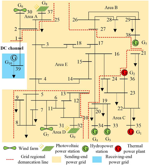
FIGURE 2. Modified 10-machine 39-bus system.

5.1 Long-term stochastic production simulation

Based on the expected scenario for each representative day of a month and the expected scenario for each day, the monthly and daily production simulations of the test system for the year to be optimized are carried out by the upper layer of the framework proposed in this paper. The generation of DC electric quantity correction in February, August and November during daily production optimization restarts the monthly production simulation respectively, and finally the DC transmission electric quantities for each month and day of the year to be optimized are obtained. The DC transmission electric quantity for each month is shown in Supplementary Figure S1. It can be seen that the overall DC transmission electric quantities from May to October are relatively big, and the electric quantity in May is the biggest in the whole year. Whereas, the monthly DC transmission electric quantities from January to April and November to December are relatively small. The electric quantity in November is the smallest in the whole year.

Taking January in the low-water period and July in the high-water period as examples, the daily UHVDC transmission electric quantity of January and July are shown in Supplementary Figures S2, S3 respectively. It can be seen that the DC transmission electric quantity difference among each day in July is small, while the difference of daily DC transmission electric quantity in January is big. The daily electric quantities in July are generally higher than those in January. The main reason is that most of the conventional units in the sending-end power grid are hydropower units, to reduce the abandoned water in high-water period, the outputs of hydropower stations are not allowed to be less than 70% of their installed capacity from May to October. Therefore, the UHVDC transmission electric quantity in the high-water period is quite different from that in the low-water period.

5.2 Short-term DRO

5.2.1 Day-ahead optimization

When execute to January 21, the day-ahead optimization is performed for January 22, and the optimization results are shown as Figure 3; Supplementary Figure S4. Compared to the daily expected scenario and the DC transmission plan in daily production simulation of January 22, the following observations can be obtained from the figures. From 9:00 to 12:00, the expected renewable energy output of the power grid at the sending-end is huge, which makes the daily optimization process in the upper layer already adjust the DC transmission power upwards according to the single maximum DC adjustment range, and there is no room for upward adjustment during the day-ahead optimization, therefore, although the day-ahead predicted renewable energy output is significantly larger than that of the expected scenario, the DC transmission results of the day-ahead optimization are still close to that of the daily production simulation. From 13:00 to 24:00, the predicted renewable energy output is greater than that of the daily expected scenario, and there is sufficient room for upward adjustment of DC transmission, so the DC transmission plan obtained from the day-ahead optimization increases compared with that of the daily production simulation, further improving the consumption of renewable energy.

FIGURE 3

FIGURE 3. Day-ahead optimization results of January 22.

When execute to June 30, the day-ahead simulation is performed for July 1, and the optimization results are shown as Figure 4; Supplementary Figure S5. In order to make full use of water resources, the hydropower units were set to the constrain of high output power during the high-water period including July 1, which makes it impossible to maintain the DC transmission plan formulated by the daily production simulation by greatly changing the output of hydropower units as in the low-water period, but more dependent on the adjustment capacity of DC transmission. Therefore, on the whole, there is a big difference between the day-ahead optimized DC transmission plan and the result of daily production simulation. When the day-ahead predicted renewable energy output decreases, the day-ahead optimized DC transmission power from 7:00 to 12:00 is still adjusted upwards compared with that of the daily production simulation. The reason is that in order to satisfy the robust chance constraints of Eqs 16, 21, it is necessary to increase the output of adjustable units during 7:00 to 9:00, so as to reserve sufficient downward adjustment capacity of units, which leads to the increase of day-ahead optimized DC transmission power. The renewable energy output is large during 10:00 to 12:00, at the same time the units have the ability to increase the output power according to the single maximum DC adjustment range at this stage, so the DC transmission power increases.

FIGURE 4

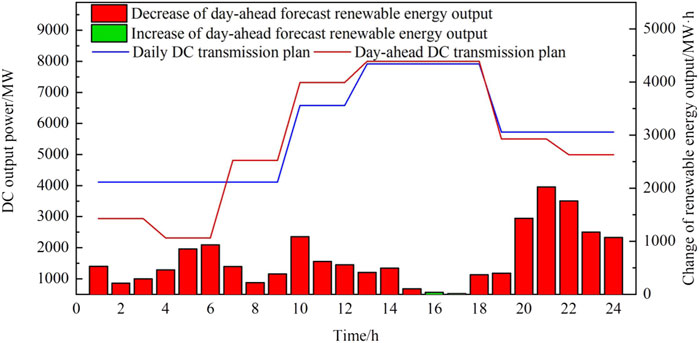
FIGURE 4. Day-ahead optimization results of July 1.

The daily electric quantity correction of UHVDC transmission in January and July are generated after the day-ahead optimization respectively, as shown in Supplementary Figures S6, S7, and then are returned to the daily production simulation. The monthly electric quantity correction of UHVDC transmission is shown in Supplementary Figure S8. By observing the monthly corrected electric quantity, we can find that the monthly electric quantity correction from January to April and November to December are all positive, and those of May to October are all negative, showing obvious characteristics of the high-water period and low-water period. In addition, the absolute electric quantity correction during the low-water period is greater than that in the high-water period, indicating that the electric quantity correction produced by day-ahead optimization during each day of the low-water period is relatively large, while it is smaller in the high-water period, which is consistent with the results in Supplementary Figures S6, S7. It can be seen that for the power grid with a high proportion of hydropower capacity, the seasonal characteristics of high-water and low-water have a great influence on renewable energy consumption and power dispatching.

5.2.2 Intra-day rolling optimization

Taking January 22 and July 1 as the examples, the intra-day rolling DRO is carried out, the optimization results for the 2 days are shown in Figure 5; Figure 6 respectively, and the adjustment factors are shown in Figure 7; Figure 8.

FIGURE 5

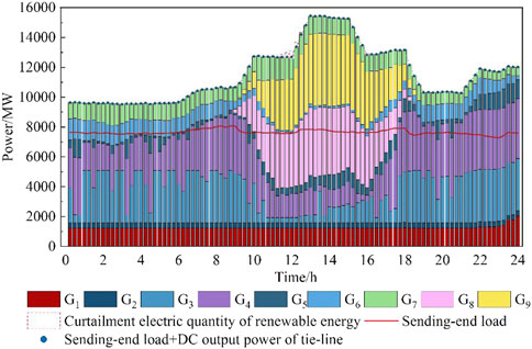
FIGURE 5. Intra-day optimization results of January 22.

FIGURE 6

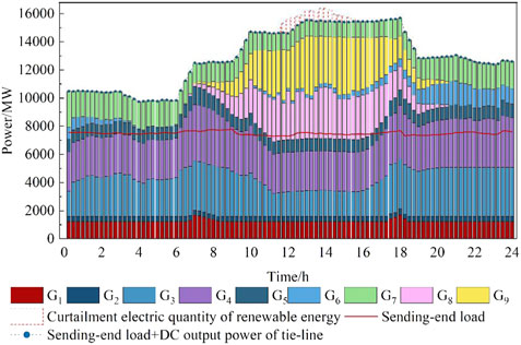
FIGURE 6. Intra-day optimization results of July 1.

FIGURE 7

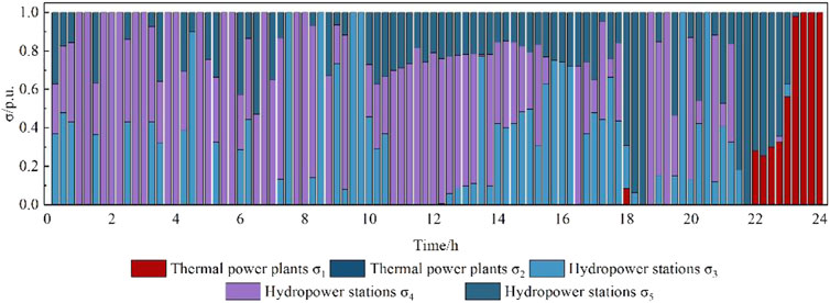
FIGURE 7. Intra-day optimization results of σ on January 22.

FIGURE 8

FIGURE 8. Intra-day optimization results of σ on July 1.

The optimization results of January 22 in Figure 5 show that: 1) From 1:00 to 8:00 and from 18:00 to 21:00, the output of renewable energies is mainly wind power, and in that period the wind power output is relatively low. So, the output of hydropower units is increased preferentially to meet the load demand of the sending-end power grid together with the DC transmission planed power. Because of the poor power supply economy, the thermal power units maintain their minimum technical output. 2) From 9:00 to 17:00, the overall output of renewable energies is at a high level due to the increasing generation of photovoltaic, in this process the thermal power units continue to maintain the minimum technical output, while hydropower units reduce their output as much as possible to increase the consumption of renewable energy. 3) From 22:00 to 24:00, the hydropower units are in full output power state. In order to cope with the decrease of wind power output, G₂ which has lower power generation costs among thermal power plants gives priority to increasing its output, and then the output of thermal power plant G₁ also increases to make up for the power shortage. 4) Some electric power from renewable energy is curtailed around 12:00, at which time the thermal power is the minimum technical output, and hydropower output also reaches the lower limit of robust constraints.

It can be seen from the intra-day optimization results of high-water period shown in Figure 6 that the hydropower units can increase their output during the low-output period of renewable energy to provide the cheap adjustment capacity, and reduce their output during the high-output period of renewable energy to promote the consumption of renewable energy. In order not to abandon water as much as possible, the hydropower units decrease their output with limit during the period that the renewable energy output is high, and increase their output when the renewable energy is low so as to meet the daily water level of the hydropower station. From 11:00 to 15:00, some electric power from renewable energy is curtailed, and at this time, both the thermal power and the hydropower units are in their minimum output state meeting the constraints.

It can be seen from Figures 7; Figure 8 that thermal power units essentially do not participate in capacity adjustment. In the high-water period, hydropower plant G₃ is the main capacity adjustment power plant. In Figure 8, G₃ is in full output power state from 20:00 to 24:00, and there is no more adjustable capacity, so hydropower plant G₄ then undertakes the capacity adjustment task.

5.3 Security analysis of the scheduling method

The risk coefficient is set to $\epsilon =0.2$, and by simulating the actual operation scenario for several times (1000 times), the ratio of the number of times that did not meet the constraints to the total number of simulations was counted as the probability of crossing the boundary to measure the operation risk. The results were shown in Table 1.

TABLE 1

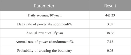
TABLE 1. Simulation results of the method in this paper.

It can be seen from the table that the probability of crossing the boundary corresponding to the method in this paper is only 0.08, far less than the risk coefficient 0.2 set in this paper. This indicates that the robust chance constraint method adopted in this paper can effectively ensure the safe operation of the high-proportion renewable energy sending-end power grid.

6 Conclusion

In this paper, a two-layer framework of multi-time scale stochastic production simulation for the optimization of UHVDC transmission is established for the sending-end power grid with a high proportion of clean energy. Referring to the energy composition and distribution of the provincial-level sending-end power grid with clean energy as its main sources in northwest China, a test system is established for verification. The research results show that: 1) Changing the daily transmission electric quantity of DC transmission line from a fixed value to a long- and short-term coordinated optimization can better adapt to the uncertainty of renewable energy output, load or system operation conditions. 2) Changing the adjustment ability of DC transmission line from traditional two-stage to multi-stage can make full use of DC transmission ability and promote the consumption of renewable energy in the power grid. 3) In the lower layer, the DRO method is adopted to deal with the randomness of renewable energy output, which improves the system operation economy while meeting certain safety requirements. 4) Taking full account of the hydropower seasonal characteristics and the storage capacity of reservoir, the adjustment ability of hydropower units can be reflected more accurately, and the renewable energy consumption and dispatching plans can be formulated more effectively. In this paper, the setting of the inter-provincial power transaction is relatively simple, and the related research will be further refined in the follow-up.

Data availability statement

The original contributions presented in the study are included in the article/Supplementary Material, further inquiries can be directed to the corresponding author.

Author contributions

All authors listed have made a substantial, direct, and intellectual contribution to the work and approved it for publication.

Funding

This paper is supported by the Science and Technology Project of State Grid Corporation of China (Research on Key Technologies of Power Grid Coordination of HVDC Send-side for All-Clean Energy Power) under SGQH0000DKJS2000124. The funder was not involved in the study design, collection, analysis, interpretation of data, the writing of this article, or the decision to submit it for publication.

Conflict of interest

HC was employed by the State Grid Zhejiang Ningbo Fenghua District Power Supply Company.

The remaining authors declare that the research was conducted in the absence of any commercial or financial relationships that could be construed as a potential conflict of interest.

Publisher’s note

All claims expressed in this article are solely those of the authors and do not necessarily represent those of their affiliated organizations, or those of the publisher, the editors and the reviewers. Any product that may be evaluated in this article, or claim that may be made by its manufacturer, is not guaranteed or endorsed by the publisher.

Supplementary material

The Supplementary Material for this article can be found online at: https://www.frontiersin.org/articles/10.3389/fenrg.2023.1075889/full#supplementary-material

References

Anstreicher, K. M. (2009). Semidefinite programming versus the reformulation-linearization technique for nonconvex quadratically constrained quadratic programming. J. Glob. Optim. 43, 471–484. doi:10.1007/s10898-008-9372-0

CrossRef Full Text | Google Scholar

Bian, Q., Xin, H., Wang, Z., Gan, D., and Wong, K. (2015). Distributionally robust solution to the reserve scheduling problem with partial information of wind power. IEEE Trans. Power Syst. 30, 2822–2823. doi:10.1109/TPWRS.2014.2364534

CrossRef Full Text | Google Scholar

Cui, Y., Li, C., Zhao, Y., Zhong, W., Wang, M., and Wang, Z. (2022). Source-grid-load multi-time interval optimization scheduling method considering wind-photovoltaic-photothermal combined DC transmission. Proc. CSEE 42, 559–573. doi:10.13334/j.0258-8013.pcsee.201907

CrossRef Full Text | Google Scholar

Delage, E., and Ye, Y. (2010). Distributionally robust optimization under moment uncertainty with application to data-driven problems. Operations Res. 58, 595–612. doi:10.1287/opre.1090.0741

CrossRef Full Text | Google Scholar

Halilbaisc, L., Pinson, P., and Chatzivasileiadis, S. (2019). Convex relaxations and approximations of chance-constrained AC-OPF problems. IEEE Trans. Power Syst. 34, 1459–1470. doi:10.1109/TPWRS.2018.2874072

CrossRef Full Text | Google Scholar

Hao, L., Ji, J., Xie, D., Wang, H., Li, W., and Asaah, P. (2020). Scenario-based unit commitment optimization for power system with large-scale wind power participating in primary frequency regulation. J. Mod. Power Syst. Clean Energy 8, 1259–1267. doi:10.35833/MPCE.2019.000418

CrossRef Full Text | Google Scholar

Li, G., Li, X., Bian, J., and Li, Z. (2021). Two level scheduling strategy for inter-provincial DC power grid considering the uncertainty of PV-load prediction. Proc. CSEE 41, 4763–4776. doi:10.13334/j.0258-8013.pcsee.200763

CrossRef Full Text | Google Scholar

Liu, Z., Zhang, Q., Dong, C., Zhang, L., and Wang, Z. (2014). Efficient and security transmission of wind, photovoltaic and thermal power of large-scale energy resource bases through UHVDC projects. Proc. CSEE 34, 2513–2522. doi:10.13334/j.0258-8013.pcsee.2014.16.001

CrossRef Full Text | Google Scholar

Lu, Z., Xu, X., Yan, Z., Wu, J., Sang, D., and Wang, P. (2020). Overview on data-driven optimal scheduling methods of power system in uncertain environment. Automation Electr. Power Syst. 44, 172–183. doi:10.7500/AEPS20200202004

CrossRef Full Text | Google Scholar

Lubin, M., Dvorkin, Y., and Backhaus, S. (2016). A robust approach to chance constrained optimal power flow with renewable generation. IEEE Trans. Power Syst. 31, 3840–3849. doi:10.1109/TPWRS.2015.2499753

CrossRef Full Text | Google Scholar

Papavasiliou, A., Oren, S., and O'Neill, R. (2011). Reserve requirements for wind power integration: A scenario-based stochastic programming framework. IEEE Trans. Power Syst. 26, 2197–2206. doi:10.1109/TPWRS.2011.2121095

CrossRef Full Text | Google Scholar

Shao, C., Feng, C., Wang, Y., Wang, X., and Wang, X. (2020). Multiple time-scale production simulation of power system with large-scale renewable energy. Proc. CSEE 40, 103–6113. doi:10.13334/j.0258-8013.pcsee.191281

CrossRef Full Text | Google Scholar

Shao, Y., Hao, L., Cai, Y., Wang, J., Song, Z., and Wang, Z. (2022). Day-ahead joint clearing model of electric energy and reserve auxiliary service considering flexible load. Front. Energy Res. 10. doi:10.3389/fenrg.2022.998902

CrossRef Full Text | Google Scholar

Sherali, H. D., and Tuncbilek, C. H. (1995). A reformulation-convexification approach for solving nonconvex quadratic programming problems. J. Glob. Optim. 7, 1–31. doi:10.1007/BF01100203

CrossRef Full Text | Google Scholar

Shu, Y., Zhang, Z., Guo, J., and Zhang, Z. (2017). Study on key factors and solution of renewable energy accommodation. Proc. CSEE 37, 1–8. doi:10.13334/j.0258-8013.pcsee.162555

CrossRef Full Text | Google Scholar

Velloso, A., Street, A., Pozo, D., Arroyo, J., and Cobos, N. (2020). Two-stage robust unit commitment for co-optimized electricity markets:an adaptive data-driven approach for scenario-based uncertainty sets. IEEE Trans. Sustain. Energy 11, 958–969. doi:10.48550/arXiv.1803.06676

CrossRef Full Text | Google Scholar

Wang, J., Shahidehpour, M., and Li, Z. (2008). Security-constrained unit commitment with volatile wind power generation. IEEE Trans. Power Syst. 23, 1319–1327. doi:10.1109/TPWRS.2008.926719

CrossRef Full Text | Google Scholar

Wang, S. J., Shahidehpour, S. M., Kirschen, D. S., Mokhtari, S., and Irisarri, G. D. (1995). Short-term generation scheduling with transmission and environmental constraints using an augmented Lagrangian relaxation. IEEE Trans. Power Syst. 10, 1294–1301. doi:10.1109/59.466524

CrossRef Full Text | Google Scholar

Wang, Z., Bian, Q., Xin, H., and Gan, D. (2017). A distributionally robust coordinated reserve scheduling model considering CVaR-based wind power reserve requirements. IEEE Trans. Sustain. Energy 7, 1–12. doi:10.1109/TSTE.2015.2498202

CrossRef Full Text | Google Scholar

Wang, Z., Lou, S., Fan, Z., Wu, Y., and Yang, Y. (2019). Chance-constrained programming based congestion dispatching optimization of power system with large-scale wind power integration. Automation Electr. Power Syst. 43, 147–154. doi:10.7500/AEPS20181219003

CrossRef Full Text | Google Scholar

Wei, W., Liu, F., and Mei, S. (2016). Distributionally robust co-optimization of energy and reserve dispatch. IEEE Trans. Sustain. Energy 7, 289–300. doi:10.1109/TSTE.2015.2494010

CrossRef Full Text | Google Scholar

Wu, H., Shahidehpour, M., Li, Z., and Tian, W. (2014). Chance-constrained day-ahead scheduling in stochastic power system operation. IEEE Trans. Power Syst. 29, 1583–1591. doi:10.1109/TPWRS.2013.2296438

CrossRef Full Text | Google Scholar

Xie, W., and Ahmed, S. (2018). Distributionally robust chance constrained optimal power flow with renewables: A conic reformulation. IEEE Trans. Power Syst. 33, 1860–1867. doi:10.1109/TPWRS.2017.2725581

CrossRef Full Text | Google Scholar

Xu, S., Wu, W., Zhu, T., and Wang, Z. (2020). Convex relaxation based iterative solution method for stochastic dynamic economic dispatch with chance constrains. Automation Electr. Power Syst. 44, 43–51. doi:10.7500/AEPS20190906001

CrossRef Full Text | Google Scholar

Zhang, H., Shen, J., Wang, G., and Hu, Y. (2022). Day-ahead two-stage stochastic optimal dispatch of AC/DC power grid considering reactive power equipment action. Automation Electr. Power Syst. 46, 133–142. doi:10.7500/AEPS20210406006

CrossRef Full Text | Google Scholar

Zhang, Y., Jiang, R., and Shen, S. (2018). Ambiguous chance-constrained binary programs under mean-covariance information. SIAM J. Optim. 28, 2922–2944. doi:10.1137/17M1158707

CrossRef Full Text | Google Scholar

Zhang, Y., Shen, S., and Mathieu, J. (2017). Distributionally robust chance-constrained optimal power flow with uncertain renewables and uncertain reserves provided by loads. IEEE Trans. Power Syst. 32, 1378–1388. doi:10.1109/TPWRS.2016.2572104

CrossRef Full Text | Google Scholar

Zhang, Z., Cheng, Y., Liu, X., and Wang, W. (2019). Two-stage robust security-constrained unit commitment model considering time autocorrelation of wind/load rediction error and outage contingency probability of units. IEEE ACCESS 7, 25398–25408. doi:10.1109/ACCESS.2019.2900254

CrossRef Full Text | Google Scholar

Zhong, H., Xia, Q., Ding, M., and Zhang, H. (2015). A new mode of HVDC tie-line operation optimization for maximizing renewable energy accommodation. Automation Electr. Power Syst. 39, 36–42. doi:10.7500/AEPS20140529005

CrossRef Full Text | Google Scholar

Zhou, A., Yang, M., Wang, M., and Zhang, Y. (2020). A linear programming approximation of distributionally robust chance-constrained dispatch with wasserstein distance. IEEE Trans. Power Syst. 35, 3366–3377. doi:10.1109/TPWRS.2020.2978934

CrossRef Full Text | Google Scholar

Zhou, A., Yang, M., Wang, Z., and Li, P. (2018). A linear solution method of generalized robust chance constrained real-time dispatch. IEEE Trans. Power Syst. 33, 7313–7316. doi:10.1109/TPWRS.2018.2865184

CrossRef Full Text | Google Scholar