Available power estimation of wind farms based on deep spatio-temporal neural networks

With the development of advanced digital infrastructure in new wind power plants in China, the individual wind-turbine level data are available to power operators and can potentially provide more accurate available wind power estimations. In this paper, considering the state of the wind turbine and the loss in the station, a four-layer spatio-temporal neural network is proposed to compute the available power of wind farms. Specifically, the long short-term memory (LSTM) network is built for each wind turbine to extract the time-series correlations in historical data. In addition, the graph convolution network (GCN) is employed to extract the spatial relationship between neighboring wind turbines based on the topology and patterns of historical data. The case studies are performed using actual data from a wind farm in northern China. The study results indicate that the computation error using the proposed model is lower than that using the conventional physics-based methods and is also lower than that using other artificial intelligence methods.

1 Introduction

In recent years, the installed capacity of wind power has gradually increased, and the proportion of new energy power generation has gradually increased. In July 2022, the Global Wind Energy Council released the “Global Wind Report 2022.” This report shows that the new installed capacity of global wind power is 93.6 GW. By the end of 2021, the cumulative installed capacity of global wind power reached 837 GW, a year-on-year increase of 12.4%. However, due to the random, fluctuating, and intermittent characteristics of wind power, it brings significant challenges to real-time dispatching of power grids (Li et al., 2019a). In this work, we focus on the available power estimation of wind farms, which refers to the theoretical power subtracting the power output of wind turbines under losses in wind farms (State Grid Corporation of China, 2018). Accurate available power is important for system operators to determine the optimal dispatch on the wind farm and other types of generators. It could also serve as an important input for many real-time monitoring and control systems.

At present, the theoretical power computation and prediction of wind farms can be divided into physics-based methods, statistics-based methods, artificial intelligence-based methods, and hybrid methods. The physics-based method mainly uses the numerical weather forecast model to calculate the future wind speed. Then, the predicted wind speed is brought into the relevant wind farm power curve (Tascikaraoglu et al., 2014) (usually provided by the wind farm manufacturer) to predict the wind farm power generations. The physical methods include the prototype machine method (Ding et al., 2016), the wind measurement tower extrapolation method (Guo et al., 2019), and the nacelle wind speed method (Jiang et al., 2014). When using the prototype method, using the prototype data to represent other wind turbine data of the same model will result in large errors. Since the wind tower extrapolation method needs to consider several factors, such as the topography, humidity, and pressure of the wind farm, the macro- and micro-climate model is very complicated. In addition, the estimation accuracy is acceptable for larger regional levels. However, for the wind farm level, it suffers from poor performance.

The statistical method is based on the statistical analysis of the correlation between wind farm power generations, wind speed, and wind direction data and establishes the mapping relationship between wind speed and wind direction and the output power of the wind farm. In the literature (Rajagopalan and Santoso, 2009), according to the actual measurement data of the wind farm, the model is based on the autoregressive moving average model (ARMA). Since ARMA can only handle stationary time series, the researchers applied the autoregressive integral moving average model (ARIMA), which can handle non-stationary time series, to wind power forecasting. However, statistical methods only analyze the superficial relationship between variables in time series. It is difficult to deal with complex and non-linear relationships.

At present, artificial intelligence-based methods are generally used for wind power forecasting and available power estimations. The artificial intelligence method uses historical power data, NWP data, etc., as input information to establish a non-linear mapping relationship between the output and multi-variables. Compared with statistical methods, the adaptability and self-learning ability of artificial intelligence methods have been significantly improved. Li et al. (2019b) used the Spearman rank correlation coefficient method to determine the hyperparameters of the long short-term memory (LSTM) network prediction model, which can effectively determine the initial step size range. Compared with the BP neural network, the wind power prediction accuracy based on the LSTM model is higher. Kisvari et al. (2021) combined the grid search method to adjust the hyperparameters of the gated recurrent unit (GRU) neural network. The proposed method achieves high accuracy with low computational cost. It shows robustness and low sensitivity to noise. The aforementioned wind power prediction methods only consider historical time-series features and do not consider complex spatial relationships. Therefore, the convolutional neural network (CNN) is used to extract the spatial features of wind farms to improve the accuracy of wind power prediction. Bai et al. (2018) redesigned the structure of CNN and proposed a temporal convolutional network (TCN). The research object of the aforementioned literature is only a single wind farm, and in most cases, regional prediction of wind power is required. Therefore, the temporal and spatial correlation between multiple wind farms needs to be further considered. Wang et al. (2022b) considered the dynamic spatio-temporal correlation between adjacent wind farms and calculated the spatio-temporal correlation matrix, modeling a graph structure with dynamic spatio-temporal correlation information as a graph convolution network (GCN) input. Experiments prove that the prediction accuracy of theoretical power generation of wind farms has been improved.

A combined model is a combination of two or more models, which eliminates the limitations of the individual models by combining their advantages in order to maximize the advantages of each method and improve the accuracy of wind farm power prediction. In a study by He et al. (2022), the weather is divided into different types according to the meteorological characteristics, and the IOWA operator is applied to assign different weight coefficients to the CNN and LSTM. The final power prediction is obtained by weighting the outputs of the two models. In a study by Liang et al. (2021), a method of CNN combined with LSTM is proposed to obtain spatial distribution characteristics of the long-term wind speed and short-term time-series characteristics. Since the CNN can only be used to process regularly arranged images, the GCN is proposed to enable feature extraction for non-Euclidean structured data. Kan and Liu (2019) used the LSTM model to extract temporal features from historical data and used the graph convolution technique to extract spatial features from multiple PV plant data in the same region. Liao et al. (2022) combined the GCN and LSTM network, adopted the GCN, captured the complex spatial correlation between adjacent wind farms through the adjacency matrix, and learned the dynamic change of the wind power curve based on LSTM. Compared with the single wind power prediction method, the combined method predicts the wind farm power with higher accuracy (Chen et al., 2021), which can retain the advantages of each model. Therefore, wind farm power prediction models based on combined methods have received extensive attention from researchers. In recent years, some scholars have adopted more advanced hybrid models, including the correlation-constrained and sparsity-controlled vector autoregressive models for spatio-temporal wind power forecasting (Zhao et al., 2018), feature extraction of meteorological factors for wind power prediction based on the variable weight-combined method (Lu et al., 2021), spatial model-based short-term wind power prediction (Ye et al., 2017), and ultra-short-term combined prediction approach based on kernel function with a specially designed switch mechanism (Peng et al., 2021).

Most of the existing wind farm power prediction methods used numerical weather forecast data or measurement data from weather towers in wind farms as model inputs and the theoretical power of the whole wind farm as the model output. Since the state of the wind turbines and the loss in the field are not taken into account, they can only be used for theoretical power generation calculation and theoretical prediction of wind farms. Few studies have been conducted to calculate the available power of wind farms.

The previous theoretical power estimation is aimed at using numerical weather forecasts to estimate the total power generated by the entire wind farm, which cannot be accurate to each wind turbine, and the error is large. The emergence of a stand-alone information system can provide the nacelle wind speed of each wind turbine so that the grid dispatching department can be based on stand-alone actual measurement data to more accurately estimate the wind turbine and wind farm available power generation. Second, in most areas of the country, the only data available to the grid dispatching department are the weather forecast data and the active power of the grid connection point, which does not include the status of waiting for wind, planned shutdown, unit failure shutdown, and other wind turbine operating conditions. However, the active power emitted by the wind turbine in the normal power generation operation state reflects the real power generation capacity of the wind turbine.

Regional control centers in China enhanced the existing SCADA system to collect each wind turbine’s operating status, wind speed, and wind direction from every wind farm, which provides an opportunity for accurate computation of available power of each wind farm. In this paper, we propose a deep spatio-temporal neural network for calculating the available power generation in wind farms based on the data to integrate wind farm’s SCADA into the control center’s SCADA. Long short-term memory (LSTM) is used to extract temporal information, and the graph convolutional network (GCN) is used to describe the topology between wind turbines in wind farms and then solve the problem of spatial correlation and station loss.

In this paper, in order to improve the prediction accuracy, based on the real-time meteorological information of each wind turbine provided by the stand-alone information system, an ultra-short-term available power calculation method is proposed. This method combines the GCN and LSTM and considers the spatio-temporal correlation of wind farms and station losses. The key contributions are as follows:

1) Stand-alone information systems are used in wind power forecasting. They can provide real-time meteorological information such as the wind speed of each wind turbine and the information on the operating status of the wind turbine.

2) A novel graph neural network-based hybrid approach is proposed for ultra-short-term power prediction. LSTM is used to excavate the temporal characteristics of the wind speed of the wind turbine. The spatial position relationship of the wind turbine constitutes graph data, which is used as an input to the GCN to capture spatial dependence.

3) Based on the construction of the electrical topology connection diagram, the station loss problem is solved in combination with the GCN.

2 Problem formulation of available power estimation of wind farms

The available power of a wind farm refers to the maximum power theoretically available from the wind energy subtracting the power output of a wind turbine under maintenance and line losses in the wind farm. Additionally, instead of the actual power output of the wind farm, it may also be subject to curtailment and dispatch signals. To estimate the maximum available power of a wind farm, the wind speed information is used as the input. In this work, we used the historical wind speed data measured at each turbine and the turbine output power data under the maximum power point tracking working condition. Therefore, the summation of power generations of all the turbines, subtracting the total losses of the wind farm, equals the maximum available power of the wind farm.

$P_{avai,i}=G\left(s_{windspeed,i}\right),(1)$

$P_{farm}={\sum }_1^n{P}_{avai,i}-P_{loss},(2)$

where $s_{windspeed,i}$ is the wind speed at the $i$^th wind turbine and $G\left(•\right)$ is the estimation method which takes the wind speed as the input and outputs the maximum power generation of the turbine. $P_{avai,i}$ is the available power of the $i$^th turbine. $n$ is the total number of turbines, and $P_{loss}$ is the loss within the wind farm. $P_{farm}$ is the estimated maximum available power of the wind farm.

The aforementioned available power calculation does not take into account the in-station losses. Since the sources of loss in the station are diverse and difficult to estimate, therefore, it is proposed to construct an electrical connection diagram of wind farm wind turbines based on the GCN using the wind farm electrical main wiring diagram, and the characteristics of the loss in the station are included in the wind turbine electrical connection diagram.

There is a correlation between the available power generation of wind turbines and the historical nacelle wind speed. The LSTM neural network layer can be constructed to effectively mine the time-series correlation information of wind turbine wind speed data. The complex topography and wake effects in the wind farm space have an impact on the power generated by the wind turbines. There is a correlation between adjacent wind turbines. Due to the different spatial distribution of WTGs and their own operating conditions, even the available power generation of WTGs of the same model varies. Therefore, based on the GCN, the fan relationship connection diagram is considered to extract spatial features.

3 The spatio-temporal NN-based algorithm for available power estimation

In terms of the structure of the proposed algorithm, in this work, a two-stage deep neural network-based algorithm is proposed, which mainly consists of four major layers. The first stage contains the first two layers, namely, the LSTM layer and the GCN layer. LSTM is a type of recurrent neural network that is proven to be very effective in terms of handling the input data with temporal relationships. The time-series wind speed data are used as the input of the LSTM layer. The GCN layer is implemented to extract the spatial topology of the wind dynamics in the wind farm to help the estimation of the available power. In the second stage, a third GCN layer is used to calculate the losses in the wind farm, where the topology of the wind farm is also used. The last layer is a fully connected layer for the final output. It should be noted that the layer here refers to a section of small network, which contains multiple sub-layers, like single GCN layers, activation function, and pooling layer. The first stage and the second stage can be pre-trained separately under the supervised learning scheme with SGD and then combined together for fine-tuning the parameters. Figure 1 shows the general framework of the proposed model, which demonstrated the structure of the proposed model. The details of the model are presented in the following sub-sections.

FIGURE 1

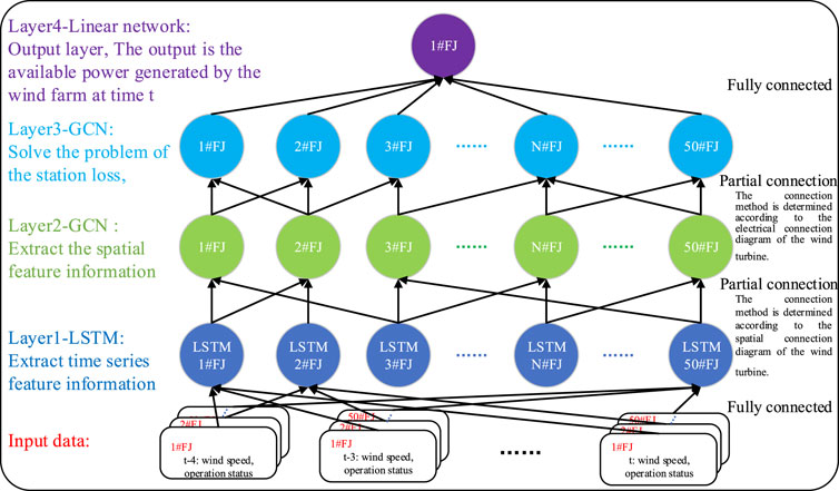
FIGURE 1. Model general frame diagram.

3.1 The correlation of time sequence extraction by the LSTM algorithm

There is a correlation between the available power generation of wind turbines and the historical nacelle wind speed (Wang et al., 2021). As a typical time series, forecasting the current wind power is not only related to forecasting the current input but also to the previous input and output. In order to fully exploit the information contained in the historical wind speed, this paper uses a long short-term memory network to extract the potential time-series information of wind turbine wind speed data for the estimation of available power generation of wind turbines.

The long short-term memory network is a variant of the recurrent neural network (RNN), which solves the problem of RNN gradient explosion and gradient disappearance. Based on the RNN, LSTM changes the single neural network layer in the RNN to one with four neural networks.

By changing the structure of neurons, LSTM introduces the gate mechanism and removes and adds information in the neurons through the gate mechanism (Hochreiter and Schmidhuber, 1997). The LSTM network can consist of one or more LSTM units that represent the data independent of each other in the time series and the data of multiple consecutive moments on the data of the current moment. The structure principle is shown in Figure 2. In Figure 2, $x_t$ represents the nacelle wind speed and the individual operating state at moment t; $h_t$ represents the power generated by the WTGs at moment t; and $c_t$ represents the effect of the power generated by the WTGs at moments t-4, t-3, t-2, and t-1 on the power generated by the WTGs at moment t.

FIGURE 2

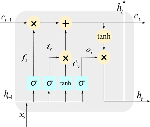
FIGURE 2. LSTM internal structure diagram.

The LSTM unit consists of four parts: information storage chain, forgetting gate, memory gate, and output gate. The information storage chain runs through all the LSTM units before and after the LSTM network and is responsible for the storage and transmission of wind speed and operation status information of wind turbines at historical moments, and the information in the information storage chain of each LSTM unit is updated. $\omega$ and $b$ denote the weight vector and offset value in each gate mechanism, respectively; $\sigma$ is the sigmoid activation function.

The role of the forgetting gate is to selectively forget the wind speed and operating status information components of some historical moments and to avoid too much information from the historical moments to affect the neural network’s processing of the wind speed and operating status inputs of the wind turbine at the current moment. By the effect of the forgetting gate, the information in the historical moments of WTGs that are not strongly correlated with the estimated moments can be eliminated. The mathematical expression of the forgetting gate is shown in Eq. 3.

$f_t=\sigma \left(W_f.\left[h_{t-1},x_t\right]+b_f\right).(3)$

The memory gate is the control unit used to control whether the wind speed and operating status data of the WTGs at time t (now) are incorporated into the network cell state. First, the $\mathit{tanh}$ function layer is used to extract the valid information from the present vector, and the output is ${\stackrel{\sim }{C}}_t$; then, the sigmoid function is used to control "how much” of this memory is to be put into the unit state, and the output is $i_t$. By using the memory gate, the strong correlation between the WTG historical moments and the estimated moments can be retained in the network cell state and passed to the next moment. The mathematical representation of the memory gate is as follows:

${\stackrel{\sim }{C}}_t=\tanh \left(W_c.\left[h_{t-1},x_t\right]+b_c\right),(4)$

$i_t=\sigma \left(W_i.\left[h_{t-1},x_t\right]+b_i\right).(5)$

The output gate integrates the output data processed by the forgetting gate and the memory gate as the output of the power generated by the wind turbine at moment t. The mathematical expression of the output gate is as follows:

$o_t=\sigma \left(W_o.\left[h_{t-1},x_t\right]+b_0\right),(6)$

$h_t=o_t*\tanh \left(C_t\right).(7)$

The network unit status is used to store information about the current WTG power, wind speed, and operating status and pass it to the next moment, which affects the output of the WTG power at the next moment. The update equation of the network unit status is shown in Eq. 8.

$C_t=f_t*C_{t-1}+i_t*{\stackrel{\sim }{C}}_{t.}(8)$

The LSTM neural network layer can be constructed to effectively mine the time-series correlation information of wind turbine wind speed data. The key historical moments of wind speed are first screened out, and then the wind speed and operation status of the key historical moments are passed into the LSTM network as input vectors, and the valid information in the key historical moments is selected through memory gates and forgetting gates to update the network unit states, thus making the LSTM network fully consider the temporal correlation when estimating the available power generation of wind turbines and thus improving the available power estimation accuracy.

3.2 The temporal correlation by the GCN algorithm

The complex topography and wake effects in the wind farm space have an impact on the power generated by the wind turbines. The wind turbines are not distributed in isolation in the wind farm space, and the data of neighboring turbines have a large contribution to the estimation of the available power generation of wind turbines. From the perspective of wind speed in wind turbine nacelle, the nacelle wind speed of a WTG at moment t in a certain wind direction has a strong correlation with the nacelle wind speed of an upstream WTG at a moment t before, and when the wind direction changes, the upstream unit of that turbine will also change. In addition, due to the different spatial distribution of WTGs and their own operating conditions, even the available power generation of WTGs of the same model varies. Therefore, in this paper, we will analyze the spatial correlation of WTGs based on the Pearson correlation coefficient of the nacelle wind speed of each WTG and construct a WTG connection relationship diagram. Then, we use a GCN to extract the spatial information within the wind farm based on the output information of the LSTM network in the previous section and establish a differentiated WTG available power generation estimation model for the wind farm.

Traditional convolutional neural networks are limited to modeling Euclidean spatial data only, while graph convolutional networks can process non-Euclidean spatial data using graph representation, which makes them more suitable for modeling all wind turbines in a wind farm. In the wind farm available power estimation, the graph data are first constructed based on the WTG connection relationship graph and the nacelle wind speed and operation status data of WTGs, and then the extraction of spatial features among WTGs is completed based on the graph convolutional neural network.

Before extracting the spatial features of wind farms using the GCN, the wind turbine connection relationship graph should be constructed based on the correlation of all wind turbines in the wind farm. Each wind turbine in the wind farm is abstracted into nodes, and the correlation of nacelle wind speed between all wind turbines in the wind farm is analyzed by the Pearson correlation coefficient, and the units with the correlation coefficient greater than the set threshold can be judged as having a correlation, and the units with a correlation are connected to form edges. Taking a wind farm with six wind turbines as an example, the connection relationship diagram of wind turbines in the wind farm is constructed, as shown in Figure 3.

FIGURE 3

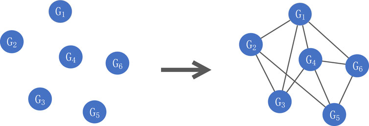
FIGURE 3. Schematic diagram of building a connection diagram of wind turbines.

The GCN is a neural network that performs feature extraction on graphs. A graph consists of a set of vertices and edges connecting the vertices [27]; the vertices are the objects studied, and the edges are specific relationships between two objects. In the wind power plant turbine connectivity graph, turbines are abstracted as nodes, and units with a strong correlation with each other constitute edges. The fan connection relationship graph notation can be expressed as $=\left(V,E\right)$, where V is the set of nodes (turbines) and E is the set of edges. The connections between turbines can be represented by the adjacency matrix $\stackrel{\sim }{A}$, and the number of edges directly connected by a given turbine is represented by the degree matrix $\stackrel{\sim }{D}$. The adjacency and degree matrices for the aforementioned example are constructed and shown in Figure 4.

FIGURE 4

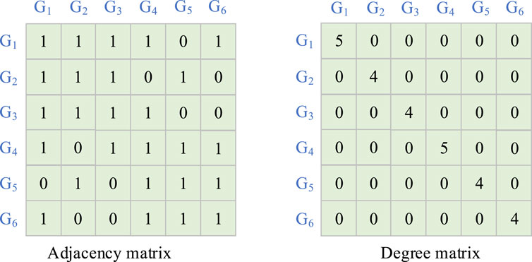
FIGURE 4. Adjacency matrix and degree matrix.

The graph convolutional neural network uses the structural information of the edge–vertex connections of the WTG connectivity graph $\stackrel{\sim }{A}$ and the input data H of each WTG to perform feature extraction of the implicit graph information. The message propagation between layers is given by Eq. 9, and the feature aggregation between turbines is given by Eq. 10.

$H^{\left(l+1\right)}=\sigma \left({\stackrel{\sim }{D}}^{-\frac{1}{2}}\stackrel{\sim }{A}{\stackrel{\sim }{D}}^{-\frac{1}{2}}{H}^{\left(l\right)}{W}^{\left(l\right)}\right),(9)$

$\begin{array}{l}{\left({\stackrel{\sim }{D}}^{0.5}\stackrel{\sim }{A}{\stackrel{\sim }{D}}^{0.5}H\right)}_i={\left({\stackrel{\sim }{D}}^{0.5}\stackrel{\sim }{A}\right)}_i{\stackrel{\sim }{D}}^{0.5}H\\ =\left({\displaystyle \sum }_k{\stackrel{\sim }{D}}_{ik}^{0.5}{\stackrel{\sim }{A}}_i\right){\stackrel{\sim }{D}}^{0.5}H\\ ={\stackrel{\sim }{D}}_{ii}^{0.5}{\displaystyle \sum }_j{\stackrel{\sim }{A}}_{ij}{\displaystyle \sum }_k{\stackrel{\sim }{D}}_{jk}^{0.5}{H}_j\\ ={\stackrel{\sim }{D}}_{ii}^{-0.5}{\displaystyle \sum }_j{\stackrel{\sim }{A}}_{ij}{\stackrel{\sim }{D}}_{jj}^{-0.5}{H}_j\\ ={\displaystyle \sum }_j\frac{1}{\sqrt{{\stackrel{\sim }{D}}_{ii}{\stackrel{\sim }{D}}_{jj}}}{\stackrel{\sim }{A}}_{ij}{H}_j\end{array}.(10)$

In Eq. 9, $H^{\left(l\right)}$ represents the input data of WTGs in the layer l network after l-1 network aggregation, $H^{\left(l+1\right)}$ represents the output data of the layer l network, n is the total number of turbines in the turbine connectivity graph, and each turbine is represented by a d-dimensional feature vector; $\stackrel{\sim }{A}=A+I_N$, where if A is multiplied directly with H, only the neighboring turbine features are considered, so it is common to add the self-loop, i.e., the unit matrix, to take into account the turbines’ own $\stackrel{\sim }{D}$, which is the degree matrix of the undirected graph, ${\stackrel{\sim }{D}}_{ii}={\sum }_j{\stackrel{\sim }{A}}_{ij}$; $W^{\left(l\right)}$ is the training parameter needed for the model and h is the output dimension; $\sigma$ is the activation function, usually ReLU or Sigmoid. After aggregation and multiplication by the weight parameter matrix, the input of the next layer of the network is obtained after the non-linear activation function $H^{\left(l+1\right)}$.

The spatial correlation problem between wind turbines can be effectively solved by using the GCN, and the schematic diagram of extracting spatial features using the GCN is shown in Figure 5. In the wind farm wind turbine connectivity graph, the initial attribute of each node, i.e., the input, is the temporal feature vector of each wind turbine extracted after LSTM. After the first layer of the GCN, the wind speed and operation status information of each wind turbine’s neighboring units are fully aggregated, and the feature vector of each node is transformed into one dimension, outputting N*1 dimensional data, so that the model considers both the temporal characteristics of the wind speed and the spatial characteristics within the wind farm, and the output of this layer is the available power generated by the wind turbine.

FIGURE 5

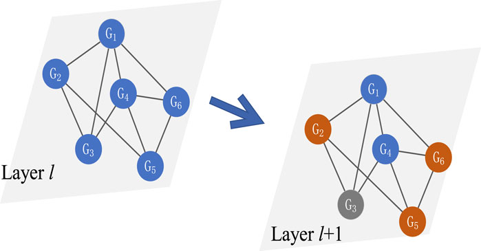
FIGURE 5. Schematic diagram of extracting spatial features by the GCN.

3.3 The station loss problem based on the layer 2 GCN algorithm

Station losses also need to be taken into account when making available power estimates. Wind turbines in the wind farm through the transformer step-up, and the power lines are connected together, and they finally go through the wind farm main transformer step-up voltage to the grid. This process will inevitably produce line losses, box transformer losses, main transformer losses, etc., which are collectively referred to as station losses. Because the station loss is not part of the power sent through the grid connection point, the station loss does not belong to the wind farm available power generation. The calculation of the wind farm available power generation needs to subtract this part of the power loss. However, station losses come from a variety of sources and are difficult to estimate, making it difficult to eliminate the impact of direct calculation on their accuracy.

Using the graph convolutional neural network, the wind turbine electrical connection relationship diagram can be constructed according to the main wind farm electrical wiring diagram, and the characteristics of the station losses are implied in the wind turbine electrical connection relationship diagram so as to indirectly complete the calculation of the losses of the convergence line, the main transformer in the wind farm. The schematic diagram of the wind turbine electrical connection relationship diagram is shown in Figure 6.

FIGURE 6

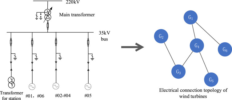
FIGURE 6. Electrical connection topology of the wind turbines.

The wind turbines are abstracted as nodes in the second layer of the GCN graph, and the power transmission paths are abstracted as edges between the nodes. The propagation process of the nodes’ own attributes in the GCN well-simulates the losses occurring in the power transmission process of the WTGs’ power generation. The input of the second GCN layer is the output matrix of the first GCN layer $H_1=R^{\left(N*l\right)}$, and the output features are the available power generation of each WTG in the wind farm, $H_2=R^{\left(N*l\right)}$. Finally, after the fully connected layer, the node characteristics of N wind turbines $H_2$ are used as the input to output the available power generated by the whole wind farm.

4 Case study

The actual operation data of a wind farm are used as an example to test the model of this paper. The installed capacity of the wind farm is 100 MW, including 50 turbines with a single capacity of 2 MW, one main transformer with a rated capacity of 120 MW, 50 box transformers with a rated capacity of 2,300 kW, and six convergence lines; the turbine models are consistent. The wind farm data include the actual power of wind turbines, wind speed, and the actual power of wind farm grid connection points, and the data sampling interval is 1 December 2020–31 December 2020, with a sampling frequency of 1 min/point and a total of 44,640 samples. To use the data more efficiently for training, testing, and validation, the 10-fold cross validation is used.

The proposed deep neural network is trained with the stochastic gradient descent (SGD) optimization algorithm and the cross-entropy loss functions. The cross-entropy loss increases as the predicted probability diverges from the actual label. A perfect model has a loss of 0. However, balancing the over and under fitting is important for the training process. Therefore, the loss will not be 0 in reality. The SGD is an iterative method for optimizing an objective function with smoothness properties. It can be considered a stochastic approximation of the conventional gradient decent optimization, where an estimated gradient is used as the replacement of the actual gradient.

In this paper, four models are compared with the proposed method. The proposed model is marked as model_1, which establishes a wind farm available output estimation model based on LSTM and GCN considering the spatial and temporal correlation within the wind farm and the loss within the wind farm; model 2 is the prototype machine method (Ding et al., 2016), and model 4 is the power curve method (Tascikaraoglu et al., 2014); model 3 considers the temporal sequence within the wind farm, based on LSTM to complete the estimation. The estimation of available power generation of wind farms is done based on LSTM (Li et al., 2019b). Model_5 is an estimation model based on LSTM and the single-layer GCN without considering in-station losses.

After the adjustment of the model structure and parameters, the parameters of the proposed model are as follows:

(1) LSTM layer: Since the input variables of the model are only the nacelle wind speed and operation status, the dimension of the input layer is 2; the number of key historical moments is determined to be 4 based on correlation analysis, so the number of time steps of the input layer is 5; for the estimation of available power generation in wind farms, this paper only considers a single-layer LSTM estimation model, so the number of hidden layer parameters is 1; the dimension of the hidden layer is generally chosen to be four times the number of input variables Therefore, the number of hidden layer dimensions of the model is 8.

(2) GCN layer: The model in this paper uses two layers of the GCN. The graph topology of the first layer network is shown in Figure 7, which is determined by the spatial correlation of WTGs, with 50 nodes and 736 edges, and the input layer dimension of each node is determined by the hidden layer dimension of LSTM, which is 8, and the output layer dimension is 1; the graph topology of the second layer network is shown in Figure 8, which is determined by the wind farm electrical connection diagram with 50 nodes and 98 edges, each of which has an input layer dimension of 1 and an output layer dimension of 1.

FIGURE 7

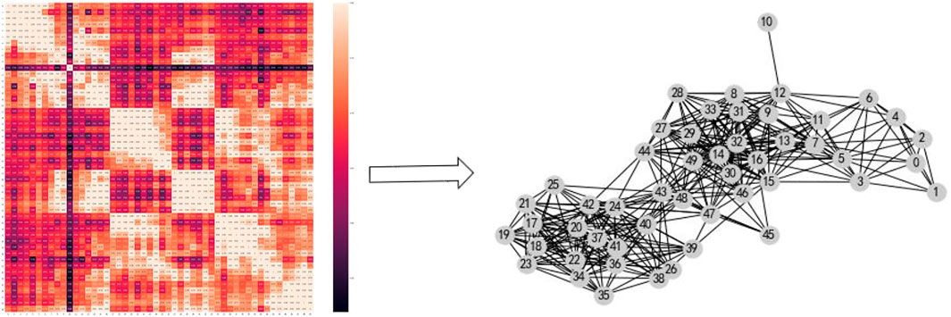
FIGURE 7. Construction of the wind farm wind turbine connection diagram.

FIGURE 8

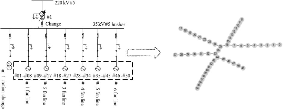
FIGURE 8. Construction of the electrical connection diagram of the wind turbine.

(3) Fully connected layer: The fully connected layer is selected as the output layer of the spatio-temporal neural network. The input layer dimension of this layer is 50, which represents the available power generation of 50 wind turbines; the output layer dimension is 1, which represents the estimated value of the available power generation of wind farms.

Based on the data of pre-processed samples completed the aforementioned four wind farm available power generation estimation models, the test set in each model estimation results is shown in Figure 9; the root mean square error and the average absolute error of the estimated value of each model and the real value are shown in Table 1.

FIGURE 9

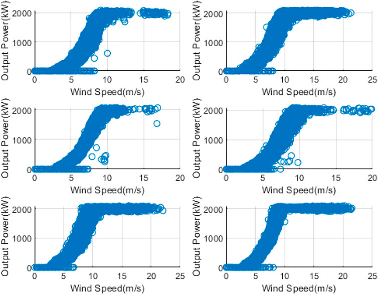
FIGURE 9. Plot of wind speed versus power output for six turbines.

TABLE 1

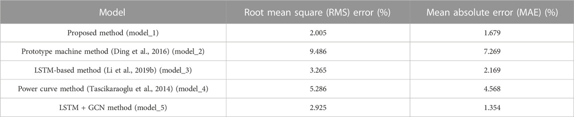
TABLE 1. Errors in the test set of the theoretical power generation estimation model for wind turbines.

In Figure 9, the original data in terms of wind speed versus output power are plotted for six different turbines. We have the data for all of the turbines in the wind farm. Due to the space limitation, only six of them are presented here. From the pattern in the figure, we can see that the maximum power of each turbine is around 2 MW. The output power of the turbines saturated around 2 MW. When the wind speed is low, in addition to the dead zone of the turbines, there are also chances that the wind turbines do not produce any power due to operation dispatches. Furthermore, the data contain outlier points due to maintenance or other reasons.

In Figure 10, the estimated power output results of the proposed method are shown for the six wind turbines. From the result, it can be seen that the proposed method can provide relatively accurate results, comparing with the real outputs.

FIGURE 10

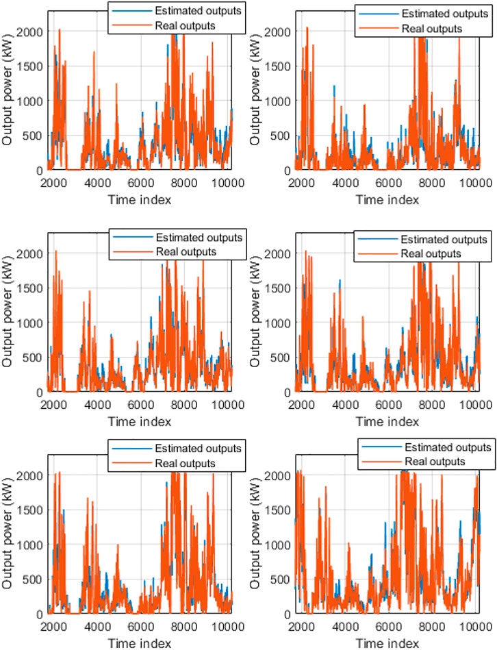
FIGURE 10. Estimated power output versus the real power outputs of the six turbines.

From Figure 11, the estimation error of model_2 is unstable and increases significantly when the wind farm is at high power generation, and the estimation error of some samples is significantly larger than that of others at low power generation, compared with the model proposed in this paper (model_1), the LSTM model (model_3), and the power curve method (model_4), which are more stable. The estimated value of the LSTM model (model_3) is lower than the real value when the wind farm is at high power generation and slightly higher than the real value when it is at low power generation. The estimated values of the proposed model (model_1) and the power curve method (model_4) are slightly higher than the true values when the wind farm is at high power generation and slightly lower than the true values when it is at low power generation. As can be seen from Figure 9, the difference between the estimated values and the true values for all the samples tested in the proposed model (model_1) is not large when the wind farm is at low power, while the difference between the estimated values and the true values for some samples of the prototype method (model_2) is small, but there are also some samples that differ significantly from the true values.

FIGURE 11

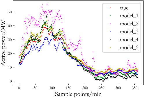
FIGURE 11. Comparison of estimated power values and real power values of a part of the test set.

From Table 1, it can be seen that the estimation error of the wind farm available power estimation model (model_1) proposed in this paper is 2.005%, and it is improved by 7.481% compared with the model_2 and by 1.26%, 3.281%, and 0.92% compared with model 3, model 4, and model_5, respectively. Model_5 adds a layer of GCN relative to model_3 to consider the spatial correlation within the wind field, reducing its root mean square error by 0.34%.

To sum up, based on the long short-term memory network and the graphical convolutional neural network, this paper establishes a model (model_1) that considers the temporal order of the wind speed of wind turbines and the spatial correlation of wind turbines inside wind farms and the station loss and has a more stable performance than that of model 2, model 3, model 4, and model_5, and its estimation error is lower and closer to the real value; by comparing model_3 and model_5 with the models proposed in this paper, it can be seen that the two-layer GCN in the model can effectively extract the spatial information inside the wind farm and solve the problem of loss in the station.

5 Conclusion

We investigate the problem of estimating the available power generation of wind farms and propose a model for calculating the available power generation of wind farms based on long short-term memory networks and graph convolutional networks.

When comparing the proposed method with the four available power generation estimation methods, namely, the sample machine method, the LSTM model, the power curve method, and the available generation power estimation method that considers only the spatio-temporal correlation method in the wind farm, the root mean square error of the proposed method is 2.138%, which is 77.5%, 34.5%, 59.6%, and 26.9% higher than that of the sample machine method, the LSTM model, the power curve method, and the method that considers only the spatio-temporal correlation within the wind farm, respectively, proving the feasibility and superiority of the proposed method.

The improvement of the accuracy of the estimation of the available power generation of wind farms will facilitate the online dispatching and optimization of the strategy of the direct wind power AGC (automatic generation control) system by the dispatching department of the State Grid Corporation, promote the consumption of new energy, and help the country achieve the reduction of carbon emissions.

In terms of the findings, limitations, and recommendations, the authors would like to share the following:

1) Due to the aerodynamics, the output power of wind farms has strong spatial correlations.

2) With the help of the data from individual turbines, more accurate estimation results in terms of available power can be generated because the state of individual turbines can be considered, including the rotating maintenance of turbines within the wind farm.

3) The performance of the machine learning algorithms is limited by the quality of the input/training dataset. Therefore, it is very important to wash and clean the dataset and find the outliers, resulting in improved estimation accuracy.

The limitation of the proposed method is also the data availability. It is fortunate that we have the data of individual wind turbines in terms of wind speed, output power, and operation states. Therefore, the model can be developed in this work, and the available power can be estimated based on individual turbine outputs and losses. Otherwise, the conventional wind forecasting is the best way to predict the output power of a wind farm.

Data availability statement

The original contributions presented in the study are included in the article/Supplementary Material; further inquiries can be directed to the corresponding author.

Author contributions

YL and PZ proposed the algorithm, KH and JL wrote the manuscript, and ZL provided valuable comments.

Funding

The work is supported by the State Grid of China, North China Branch, under Project No. SGNCOOOODKJS2000265.

Conflict of interest

Author YL was employed by North China Branch of the State Grid Corporation of China.

The remaining authors declare that the research was conducted in the absence of any commercial or financial relationships that could be construed as a potential conflict of interest.

Publisher’s note

All claims expressed in this article are solely those of the authors and do not necessarily represent those of their affiliated organizations, or those of the publisher, the editors, and the reviewers. Any product that may be evaluated in this article, or claim that may be made by its manufacturer, is not guaranteed or endorsed by the publisher.

References

Bai, S., Kolter, J. Z., and Vjapa, Koltun (2018). An empirical evaluation of generic convolutional and recurrent networks for sequence modeling. arXiv:1803 https://arxiv.org/abs/1803.01271.

Google Scholar

Chen, H., Birkelund, Y., and Yuan, F. J. E. R. (2021). Examination of turbulence impacts on ultra-short-term wind power and speed forecasts with machine learning. Energy Rep. 7, 332–338. doi:10.1016/j.egyr.2021.08.040

CrossRef Full Text | Google Scholar

Ding, Kun, Qingquan, Lü, and Xu, Cai (2016). Statistical analysis of measured data on the calculation of wind farm curtailed wind power by model machine method. Renew. energy 1, 56–63.

Google Scholar

Focken, U., Lange, M., and Waldl, H. P. (2001). “Previento-a wind power prediction system with an innovative upscaling algorithm,” in Proceedings of the European Wind Energy Conference, Copenhagen, Denmark, 276.

Google Scholar

Fu, Yang, Ren, Zixu, Shurong, Wei, Wang, Yang, Huang, Lingling, and Jia, Feng (2022). Ultra-short-term power prediction of offshore wind power based on improved LSTM-TCN model. Chin. J. Electr. Eng. 12. doi:10.13334/j.0258-8013.pcsee.210724

CrossRef Full Text | Google Scholar

Guo, Haisi, He, Hui, and Bao, Daen (2019). Theoretical power generation calculation and comparative optimization of wind turbines. Electr. Power Energy 40 (3), 339–343.

Google Scholar

He, B., Ye, L., Pei, M., Lu, P., Dai, B., and Li, Z. (2022). A combined model for short-term wind power forecasting based on the analysis of numerical weather prediction data. Energy Rep. 8, 929–939. doi:10.1016/j.egyr.2021.10.102

CrossRef Full Text | Google Scholar

Hochreiter, S., and Schmidhuber, J. (1997). Long short-term memory. Neural Comput. 9 (8), 1735–1780. doi:10.1162/neco.1997.9.8.1735

PubMed Abstract | CrossRef Full Text | Google Scholar

Jiang, Wenling, Feng, Shuanglei, and Sun, Yong (2014). Research on the calculation method of abandoned wind power in wind farms based on wind speed data of engine room. Power Grid Technol. 38 (3), 647–652. doi:10.13335/j.1000-3673.pst.2014.03.016

CrossRef Full Text | Google Scholar

Kan, Bowen, and Liu, Guangyi (2019). Prediction of distributed photovoltaic power generation based on graph machine learning. Power Supply 36 (11), 20–27. doi:10.19421/j.cnki.1006-6357.2019.11.003

CrossRef Full Text | Google Scholar

Kisvari, A., Lin, Z., and Liu, X. J. R. E. (2021). Wind power forecasting–A data-driven method along with gated recurrent neural network. Renew. Energy 163, 1895–1909. doi:10.1016/j.renene.2020.10.119

CrossRef Full Text | Google Scholar

Li, J., Geng, D., Zhang, P., Meng, X., Liang, Z., and Fan, G. “Ultra-short term wind power forecasting based on LSTM neural network,” in Proceedings of the 2019 IEEE 3rd International Electrical and Energy Conference (CIEEC), Beijing, China, September 2019 (IEEE).

Google Scholar

Li, K., Zhang, P., Li, G., Wang, F., Mi, Z., and Chen, H. J. I. A. (2019). Day-ahead optimal joint scheduling model of electric and natural gas appliances for home integrated energy management. IEEE Access 7, 133628–133640. doi:10.1109/access.2019.2941238

CrossRef Full Text | Google Scholar

Liang, Chao, Liu, Yongqian, Zhou, Jiakang, Yan, Jie, and Lu, Zongxiang (2021). Multi-point wind speed prediction method in wind farm based on convolutional recurrent neural network. Power Grid Technol. 45 (2), 534–542. doi:10.13335/j.10003673.pst.2020.0767

CrossRef Full Text | Google Scholar

Liao, W., Bak-Jensen, B., Pillai, J. R., Yang, Z., and Liu, K. J. E. P. S. R. (2022). Short-term power prediction for renewable energy using hybrid graph convolutional network and long short-term memory approach. Electr. Power Syst. Res. 211, 108614. doi:10.1016/j.epsr.2022.108614

CrossRef Full Text | Google Scholar

Liu, Zhongyu, Li, Yanlin, and Zhou, Yang (2020). Graph neural networks: Analysis of GNN principles. Beijing, China: Machinery Industry Press.

Google Scholar

Lu, P., Ye, L., Zhao, Y., Dai, B., Pei, M., and Li, Z. (2021). Feature extraction of meteorological factors for wind power prediction based on variable weight combined method. Renew. Energy 179, 1925–1939. doi:10.1016/j.renene.2021.08.007

CrossRef Full Text | Google Scholar

Peng, L. A., Lin, Y. A., Yong, T. B., Yz, A., Wz, B., and Ying, Q. C. (2021). Ultra-short-term combined prediction approach based on kernel function switch mechanism. Renew. Energy 164, 842–866. doi:10.1016/j.renene.2020.09.110

CrossRef Full Text | Google Scholar

State Grid Corporation of China, (2018). Calculation method of wind power theoretical power and blocked power: Q/Gdw 11900-2018. Beijing: State Grid Corporation of China

Google Scholar

Rajagopalan, S., and Santoso, S. “Wind power forecasting and error analysis using the autoregressive moving average modeling,” in Proceedings of the IEEE Power & Energy Society General Meeting, Calgary, AB, Canada, July 2009.

Google Scholar

Tascikaraoglu, A., Uzunoglu, M. J. R., and Reviews, S. E. (2014). A review of combined approaches for prediction of short-term wind speed and power. Renew. Sustain. Energy Rev. 34, 243–254. doi:10.1016/j.rser.2014.03.033

CrossRef Full Text | Google Scholar

Wang, Y., Zou, R., Liu, F., Zhang, L., and Liu, Q. (2021). A review of wind speed and wind power forecasting with deep neural networks. Applied Energy 304, 117766. doi:10.1016/j.apenergy.2021.117766

CrossRef Full Text | Google Scholar

Wang, F., Chen, P., Zhen, Z., Yin, R., Cao, C., and Zhang, Y. (2022). Dynamic spatio-temporal correlation and hierarchical directed graph structure based ultra-short-term wind farm cluster power forecasting method. Appl. Energy 323, 119579. doi:10.1016/j.apenergy.2022.119579

CrossRef Full Text | Google Scholar

Wang, L., He, Y., Liu, X., Li, L., and Shao, K. J. E. R. (2022). M2TNet: Multi-modal multi-task Transformer network for ultra-short-term wind power multi-step forecasting. Energy Rep. 8, 7628–7642. doi:10.1016/j.egyr.2022.05.290

CrossRef Full Text | Google Scholar

Ye, L., Zhao, Y., Zeng, C., and Zhang, C. (2017). Short-term wind power prediction based on spatial model. Renew. energy 101 (4), 1067–1074. doi:10.1016/j.renene.2016.09.069

CrossRef Full Text | Google Scholar

Zeiler, A., Brooks, D., Blau, G., and Pekny, J. (2011). Elsevier, Improved wind power forecasting with ARIMA modelsComput. Aided Chem. Eng., 29 1789–1793.

Google Scholar

Zhao, Y., Ye, L., Pinson, P., Tang, Y., and Lu, P. (2018). Correlation-constrained and sparsity-controlled vector autoregressive model for spatio-temporal wind power forecasting. IEEE Trans. Power Syst. 33, 5029–5040. doi:10.1109/tpwrs.2018.2794450

CrossRef Full Text | Google Scholar