Research on the state of health estimation of lithium-ion batteries for energy storage based on XGB-AKF method

With the advantages of high energy density, long cycle life and high stability, lithium-ion batteries have been used in a large number of fields such as electric vehicles and grid scale energy storage. To ensure the safe and reliable operation of battery systems, it is important to make an accurate and rapid estimation of the state of health (SOH) of Li-ion cells. A Li-ion cell is a complex nonlinear dynamic system. The SOH of a Li-ion can not be measured directly in actual working conditions; it can only be estimated indirectly by external characteristic parameters that reflects the extent of cell aging. It is difficult to ensure the reliability of method based on a single aging feature or model. Therefore, this paper proposes a multi-feature SOH estimation method that combines data-driven XGBoost and a Kalman filter. Firstly, a principal component analysis algorithm to reconstruct multiple battery aging features based on data is used, and an XGBoost online estimation model incorporating multiple features based on the reconstructed feature data is constructed. Finally, the joint optimal estimation of SOH of Li-ion cells by introducing a time-domain Kalman filter based on the real-time correction of the XGBoost model is achieved in this method. The results show that the method improves the accuracy and robustness of the estimation model and achieves a high-precision joint estimation of SOH for Li-ion cells.

1 Introduction

The standard definition of the state of health (SOH) of a cell is the ratio of the current capacity to the nominal capacity of the cell (Yang et al., 2022). The SOH of a new cell is 100%, which decreases continually with the continuous decline in the cycle performance of the cell. According to IEEE standards, a cell has been aged and cannot be used when the SOH drops to 80%, which should be replaced timely. SOH indicators serve as an important parameter for battery management systems (BMSs) and fault detection, and SOH estimation plays an important role in improving cell life and ensuring system safety (Berecibar et al., 2016; Li et al., 2021). With the rapid development of large-scale battery energy storage stations, the functions of such enhanced BMS need to be improved (Carkhuff et al., 2018). At present, SOH estimation is the weak point of the BMSs, which directly affects the efficiency, safety, and reliability of the Li-ion cell usage.

As one of the core parameters of BMSs, the main methods for SOH estimation can be divided into three categories: direct measurement methods, model-based methods and data-driven methods (Xiong et al., 2018; Tan et al., 2022). Each of the three categories contain multiple specific methods as shown in Figure 1. The direct measurement method estimates the SOH by experimentally measuring the maximum capacity or internal resistance of the cell (Waag et al., 2013; Gholizadeh and Yazdizadeh, 2020). The capacity measurement is usually carried out by charging and discharging the Li-ion cell at 100% depth under specific standard operating conditions, and the cell capacity is obtained by the Ampere counting method. The model-based methods mainly include the electrochemical model and the Equivalent circuit models ECM (Lai et al., 2020). The electrochemical modelling method has a high accuracy and is built from the molecular level perspective of the internal reaction mechanism of the cell, providing insight into its internal microscopic working mechanism. The ECM is built from the perspective of a circuit, which is composed of an ideal voltage source, a capacitor, resistor, and constantphase elements, and it is used to describe the behavior of nonideal electric double layer capacitors (Chen and Wang, 2014; Shi et al., 2021). The data-driven methods treat the cell as a black box, eliminating the need to study its complex chemistry and internal structure (Jain et al., 2021). These methods mine aging information from historical operation data and achieve the SOH estimation of a new cell by using the pre-trained model. The direct measurement methods are usually used in calibrating the true value of SOH. The estimation accuracy of the direct measurement is not satisfactory due to the single aging characteristic and high equipment accuracy requirement. However, the electrochemical modelling method have high complexity, and contains a large number of parameters that cannot be measured externally (Zhang et al., 2022). Therefore, the electrochemical modelling method is generally used in the laboratory for theoretical research and are hardly applied in practical engineering.

FIGURE 1

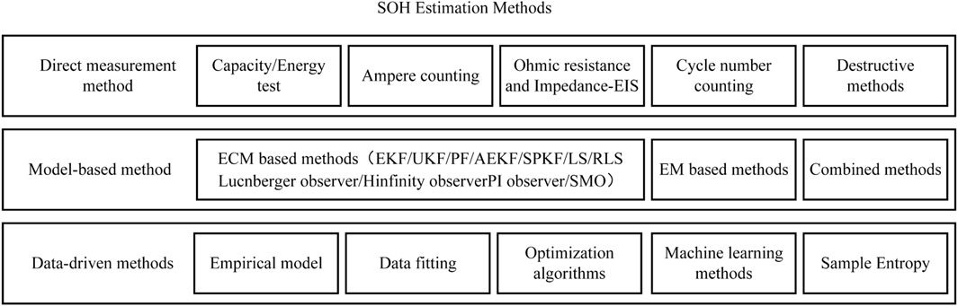
FIGURE 1. Classification of SOH estimation methods.

At present, research on the SOH estimation method of lithium-ion cells is not sufficient: the aging characteristics of lithium-ion cells are relatively single, and the reliability and accuracy of the model requires improvement. Data-driven methods establish an estimation model based on data through statistical laws, so as to establish a nonlinear mapping relationship between the external cell characteristics parameters and the SOH. These methods effectively avoid the complexity of the model building and have ideal estimation accuracy and practicality, making them the most ideal methods for estimating the SOH at present (Chang et al., 2021). The limitations of data-driven methods are an excessive dependence on historical data and a lack of model variation with structural time series trends. The prediction results of such methods may be affected by the uncertainty of the data. Therefore, more in-depth research is necessary to improve the reliability of the parameters characterizing the SOH. In summary, it is important to find an accurate and fast method for estimating the SOH of lithium-ion cells to improve the safety and reliability of battery energy storage systems.

With the improvement’ of computer hardware, the emergence of artificial intelligence algorithms, and the advent of the era of big data, data-driven methods have gradually become the mainstream research direction. Machine learning as a data-driven method to achieve artificial intelligence has been widely used in various fields in recent years, which only needs to monitor the battery voltage and current data to achieve a battery SOH estimation. For example, machine learning applications such as autoregressive models, Gaussian process regression, support vector machines, and neural networks have been applied to the prediction of battery SOH and remaining service life (Widodo and Yang, 2011; Liu et al., 2013; Long et al., 2013; Klass et al., 2014), and good results have been achieved.

By improving the data-driven estimation model, this paper combines XGBoost and adaptive Kalman filter to learn from each other’s strengths. In this paper, the XGBoost algorithm is used to build a data-driven online estimation model, and the Kalman filter is introduced to correct the adverse effects of historical data on the XGBoost model by using its state equation based on time-domain recursion. A data validation analysis shows that the method improves the accuracy and robustness of the model, making the final estimation results smoother and more accurate.

The rest of this paper is organized as follows. In the second section, the relevant principles about the Kalman filter and the adaptive filter are introduced. The third section investigates the XGB-AKF-based SOH estimation method for lithium-ion cells for battery energy storage and verifies the accuracy of the method through experiments. The fourth section summarizes the entirety of this study.

2 Introduction of related principles

2.1 XGBoost algorithm

The XGBoost algorithm is an optimization algorithm proposed by Chen at the University of Washington in 2015 based on the idea of gradient boosting, which has gained widespread attention due to its excellent learning ability and efficient learning speed. The weighted quantile method in the XGBoost algorithm (used to search for the approximate optimal split point), parallel and distributed computing, and efficient and fast processing methods for large amounts of data based on chunking technology have led to significant improvements in the computational speed and prediction accuracy of the model. A sparse perception algorithm based on decision trees can automatically learn the splitting direction for samples with missing feature values, which improves the accuracy of estimation results in the case of missing features in the test set. XGBoost, in comparison with GBDT and AdaBoost, avoids the model overfitting problem and improves the adaptability of the model due to the inclusion of the regularization-oriented structural loss function as the optimization objective function.

The XGBoost algorithm used in this paper uses integrated learning based on CART regression trees, which use the Gini index to select the segmentation features. The Gini index is the probability that a randomly selected sample is misclassified in the sample data. The magnitude of the Gini index indicates the probability that the selected sample is misclassified. The smaller the value, the higher the purity of the set; in other words the Gini index (Gini impurity) is equal to the probability that the sample is selected multiplied by the probability that the sample is misclassified. The equation for the Gini coefficient is shown below (Jing-tai and Wang., 2022).

$\begin{array}{c}Gini\left(p\right)={\sum }_{k=1}^K{p}_k\left(1-p_k\right)=1-{\sum }_{k=1}^K{p_k}^2\end{array}(1)$

where $p_k$ denotes the probability that the selected sample belongs to category k. The probability that the sample is misclassified is (1-$p_k$).

For a sample set D the Gini index is (FEI Chen et al., 2022):

$\begin{array}{c}Gini\left(D\right)=1-{\sum }_{k=1}^K{\left(\frac{\left|C_k\right|}{\left|D\right|}\right)}^2\end{array}(2)$

A feature (A) is divided into v subsets $\left(D_1,D_2,\dots ,D_v\right)$ by v different values, and the value with the smallest Gini index (i.e., the largest information gain) is determined to be the splitting point. Then, the Gini index of feature A is related to data set D as in Eq. 3 (Ma and Cheng, 2022):

$\begin{array}{c}Gini\left(D,A\right)={\sum }_{y=1}^V\frac{\left|D^v\right|}{\left|D\right|}Gini\left(D^v\right)\end{array}(3)$

The feature that minimizes the Gini index of the sample is used as the attribute of the split node when building the regression decision tree. For an arbitrary division of data for feature A, suppose the corresponding division point (s) is divided into data sets $D_1$ and D2 on both sides, and the feature and eigenvalue division point that minimizes the Gini index of the respective sets of $D_1$ and $D_2$, while the Gini index of $D_1$ and $D_2$ is minimized, is selected. The expression is as follows.

$\begin{array}{c}\min \left[{\mathit{min}}_{c1}{\sum }_{x_i\in D_1\left(A,s\right)}{\left(y_i-c_1\right)}^2+{\mathit{min}}_{c2}{\sum }_{x_i\in D_2\left(A,s\right)}{\left(y_i-c_2\right)}^2\right]\end{array}(4)$

where c1 is the sample output mean of dataset $D_1$ and c2 is the sample output mean of dataset $D_2$. We then iterate through the feature variables and scan cut point s for fixed feature A, select the best cut point (A, s) that minimizes the value of Eq. 4, and calculate the corresponding leaf node output values (c1,c2) to get two sub-regions $(D_1$, $D_2)$. We continue to traverse the feature variables to divide the subregions until either the number of samples is less than the threshold or there are no features. Finally, the input samples are divided into m subregions $\left(D_1{,D}_2,\dots ,D_m\right)$ to generate the decision tree:

$\begin{array}{c}f\left(x\right)={\sum }_{m=1}^M{c}_{m}I\left(x\in D_m\right)\end{array}(5)$

At the core of the XGBoost algorithm is a Boosting optimization model based on decision trees, which combines weak learners into strong learners through iteration. XGBoost uses CART regression trees as weak learners, first determines the optimal structure of the tree (number of leaf nodes, depth), and adopts a stepwise forward additive model; in each generation of a single tree, the weight of the data from the previous division of error is adjusted upward before acting on the current tree. The overall error of the model is gradually reduced by continuously adding trees until the end of training. XGBoost training is performed for each tree, whose model can be written as follows:

$\begin{array}{c}{f}_t\left(x\right)=w_{q\left(x\right)},w\in R^T,q:R^d\left\{\mathrm{1,2},\cdots T\right\}\end{array}(6)$

where $w$ is the leaf node score. $x$ denotes the input sample data, $q\left(x\right)$ denotes the leaf node corresponding to sample $x$, and $T$ is the number of leaf nodes in the tree. The formula for adding thet^th

Tree to the model is as follows.

$\begin{array}{c}{\widehat{y}}_i^{\left(t\right)}={\displaystyle \sum }_{k=1}^t{f}_k\left(x_i\right)={\widehat{y}}_i^{\left(t-1\right)}+f_t\left(x_i\right)\end{array}(7)$

For the training of a single CART tree it is first necessary to determine the objective function.

$\begin{array}{c}Obj\left(\theta \right)={\displaystyle \sum }_{i=1}^{n}L\left(y_j,{\widehat{y}}_i^{\left(t\right)}\right)+{\displaystyle \sum }_{k=1}^t\Omega \left(f_K\right)\end{array}(8)$

The objective function is divided into two parts: a loss function (L) and a regularization term $\left(\Omega \right)$. As a regression problem the loss function is usually chosen as L2 loss (i.e., the square of the residuals between the predicted and true values) to evaluate the degree of model fit, and the regularization term is used to penalize the complexity of the model to prevent overfitting. The regularization term is defined as follows (CHAI et al., 2022).

$\begin{array}{c}\Omega \left(f_t\right)=rT+\frac{1}{2}\lambda {\Sigma }_{j=1}^T{w}_j^2\end{array}(9)$

where $T$ is the number of leaf nodes, $w_j$ is the L2 norm for the fraction of leaf nodes, and $r$ and $\lambda$ are used as parameters to control the tree complexity. From this expression, the regularization term can be calculated, and then Eqs 6 and Eqs 7 are included in the objective function and expanded using the second-order Taylor formula to obtain the tth tree leaf node form (Wu et al., 2022).

${Obj}^t\left(\theta \right)={\displaystyle \sum }_{i=1}^n\left[g_i{w}_{q\left(x_i\right)}\frac{1}{2}{h}_i{w}_{q\left(x_i\right)}^2\right]+\frac{1}{2}\lambda {\displaystyle \sum }_{j=1}^T{w}_j^2$

$={\displaystyle \sum }_{j=1}^T\left[\left({\displaystyle \sum }_{\mathrm{i}\in I_j}{g}_i\right)w_j+\frac{1}{2}\left({\displaystyle \sum }_{\mathrm{i}\in I_j}{h}_i+\lambda \right)w_j^2\right]+rT(10)$

We let $G_j={\displaystyle \sum }_{\mathrm{i}\in I_j}{g}_i$ and $H_j={\displaystyle \sum }_{\mathrm{i}\in I_j}{h}_i$ Bringing into Eq. 10 and taking the partial derivative of the objective function with respect to w_j and making the derivative function zero, we solve for w_j:

$\begin{array}{c}{w}_j^{*}=-\frac{G_j}{H_j+\lambda }\end{array}(11)$

Plugging Eq. 11 into the objective function yields the following expression:

$\begin{array}{c}{Obj}^{*}=-\frac{1}{2}{\displaystyle \sum }_{j=1}^T\frac{G_j^2}{H_j+\lambda }+rT\end{array}(12)$

${Obj}^{*}$ serves as a criterion to evaluate the structure of a single CART regression tree, and XGBoost enumerates the splitting schemes of all features starting from the tree with depth 0 and calculates their objective function values to determine the optimal structure of the tree. When the tree reaches the maximum depth, the sum of sample weights is less than the set threshold (i.e., too few samples of leaf nodes), and the model stops building the decision tree. The proportion of samples drawn from each tree is controlled by the set parameters, and the optimal structure of a tree is finally trained by adjusting the parameters.

XGBoost uses Boosting for the next round of training after a tree is trained (the objective function of the next tree contains the previous prediction results), and the optimal model structure is obtained through iteration. XGBoost multiplies the weights of the leaf nodes by the learning rate after one iteration to weaken the influence of each tree and allow more learning space forlater trees. Finally, the optimal number of model iterations is determined, namely, the number of decision trees need to complete the training of the model.

2.2 Kalman filtering principle

The Kalman filter algorithm constructs a state equation describing the linear system and substitutes the observation data of the system input and output into Eequation 13) for prediction and correction, so as to achieve the optimal estimation of the system state (Sinopoli et al., 2004). The core of the Kalman filter algorithm is to recursively update the estimates through a series of recursive equations combined with the observed parameters. The discrete state equations describing the linear system are first established as follows (Li et al., 2020).

$\begin{array}{c}\{\begin{array}{c}{x}_{k+1}=A_k{x}_k+B_k{u}_k+w_k\\ z_k=C_k{x}_k+D_k{u}_k+v_k\end{array}\end{array}(13)$

where $x_k$ is the system state variable, $z_k$ is the observed variable, and $w_k$ and $v_k$ denote the system state noise and the observed noise, respectively. $w_k$ and $v_k$ are mutually independent Gaussian white noise with zero mean. The variances of $w_k$ and $v_k$ are Q and R, respectively. $u_k$ is the external input to the system, which is zero when there is no external input.

The Kalman filter substitutes the optimal state estimate at the previous moment into the system state equation to derive the a priori state estimate, and it uses the Kalman gain to record the measured values at one moment in the a posteriori estimate at the next moment by multiplying them after obtaining the observed values. That is, the posterior estimate at a certain time is the maximum probability obtained by weighing the posterior estimate at the previous time and the current observation value. Thus, the current posterior estimate is an optimization of the prior estimate. The Kalman filter expresses the error between the estimated and true values in terms of the covariance $\left(P_k\right)$ as follows (Yan, 2016):

$\begin{array}{c}{P}_k=E\left[\left(x_{\mathrm{k}}-x_{\mathrm{k}}^{+}\right){\left(x_{\mathrm{k}}-x_{\mathrm{k}}^{+}\right)}^T\right],\end{array}(14)$

where $x_k$ denotes the true value of the parameter to be measured, and $x_{\mathrm{k}}^{+}$ denotes the estimated value at the kth moment.

The specific iterative steps of the Kalman filtering algorithm are as follows (Zhu and He, 2019):

1) System initialization:

$\begin{array}{c}\{\begin{array}{c}{x}_0^{+}=E\left[x_0\right]\\ P_0^{+}=E\left[\left(x_0-x_0^{+}\right){\left(x_0-x_0^{+}\right)}^T\right]\end{array}\end{array}(15)$

2) A priori state estimation:

$\begin{array}{c}{x}_k^{-}=A_{k-1}{x}_{k-1}^{+}+B_k{u}_{k-1}\end{array}(16)$

3) Error covariance a priori estimation:

$\begin{array}{c}{P}_k^{-}=A_{k-1}{P}_{k-1}^{+}{A}_{k-1}^T+Q\end{array}(17)$

4) Calculate the Kalman gain:

$\begin{array}{c}{K}_k=P_k^{-}{C}_k^T{\left[C_k{P}_k^{-}{C}_k^T+R\right]}^{-1}\end{array}(18)$

5) System status update:

$\begin{array}{c}{x}_k^{+}=x_k^{-}+K_k\left(z_k-C_k{x}_k^{-}-D_k{u}_k\right)\end{array}(19)$

6) Posterior covariance estimates:

$\begin{array}{c}{P}_k^{+}=P_k^{-}\left(I-K_k{C}_k\right)\end{array}(20)$

7) k = 2,3,4... Repeat steps 2–6 recursively.

The Kalman filter algorithm is widely used in parameter estimation, which estimates system state $x_k^{-}$ at moment k under system state $x_{k-1}^{+}$ and system input $u_{k-1}$, calculates the optimal estimate $x_k^{+}$ by combining the current observation $z_k$, filters the Gaussian white noise in the data, and quickly tracks the changes of the state and parameters.

2.3 Adaptive filtering principle

The Sage-Husa-based adaptive Kalman filter (AKF) is composed of two parts: the classical Kalman filter algorithm and a noise estimator. The adaptive adjustment process refers to the real-time correction of system errors and observation errors through the time-varying noise statistical estimator during the iterative state-updating process of the Kalman filter, so as to reduce noise interference and improve model accuracy (Myers and Tapley, 1976; Oldham, 2008). The AKF equation is as follows (Garcia et al., 2019):

$\begin{array}{c}\{\begin{array}{c}{x}_k=A_{k-1}{x}_{k-1}+B_{k-1}{u}_{k-1}+q_{k-1}\\ z_k=C_{k-1}{x}_{k-1}+D_{k-1}{u}_{k-1}+r_{k-1}\end{array}\end{array}(21)$

And the AKF noise estimator is as follows (Zhu and He, 2019):

$\begin{array}{c}{e}_k=z_k-H_{k-1}{x}_{k-1}-r_{k-1}\end{array}(22)$

$\begin{array}{c}{r}_k=\left(1-d_{k-1}\right)r_{k-1}+d_{k-1}\left(z_k-H_k{x}_{k-1}\right)\end{array}(23)$

$\begin{array}{c}{q}_k=\left(1-d_{k-1}\right)q_{k-1}+d_{k-1}\left(x_k-A_k{x}_{k-1}\right)\end{array}(24)$

$\begin{array}{c}{Q}_k=\left(1-d_{k-1}\right)Q_{k-1}+d_{k-1}\left(K_k{e}_k{e}_k^T{K}_k^T+P_k-A_k{P}_k{A}_k^T\right)\end{array}(25)$

$\begin{array}{c}{R}_k=\left(1-d_{k-1}\right)R_{k-1}+d_{k-1}\left(e_k{e}_k^T-H_k{P}_k{H}_k^T\right)\end{array}(26)$

$\begin{array}{c}{d}_k=\frac{\left(1-b\right)}{\left(1-b^{k-1}\right)}\end{array}(27)$

where $r_k$ represents the observed noise mean, $q_k$ represents the system noise mean, $R_k$ represents the observed noise variance, and $Q_k$ represents the system noise variance. The noise estimator is added to the Kalman filter iterative algorithm by the time-varying noise-extreme a posteriori estimator to dynamically update the noise variance $r_{k+1},q_{k+1},R_{k+1}$ and $Q_{k+1}$ simultaneously after the kth iteration of the filter. $d_k$ in Eq. 27 denotes the forgetting factor, which is used to reduce the impact of longer time data on the current $r_k,q_k{,R}_k,\mathrm{a}\mathrm{n}\mathrm{d}{Q}_k$ and enhance the impact of data in the nearer moments. The forgetting factor takes the value range of 0 < b < 1 and is usually set between 0.95 and 0.99, which not only aggravates the most recent observations but also limits the memory length of the filter. The introduction of the forgetting factor can regulate the weight of the observations at different moments of the system. The Sage–Husa-based AKF continuously adapts to the changes of system parameters by adjusting the weights to reduce the model estimation error.

2.4 Principal component analysis

Principal component analysis (PCA) is a multivariate statistical method that converts n-dimensional features of data into k-dimensional new orthogonal features by an orthogonal transformation according to the maximum variance theory. The reconstructed k-dimensional features retain most of the information in the original data and are uncorrelated with each other, and PCA minimizes information loss while compressing the data. PCA is often used in data analysis and processing for data dimensionality reduction, which can maximize the simplification of attributes within the specified loss range, remove the redundant interference of strong correlation between features on the training process, and improve the model training speed and accuracy.

The specific steps of PCA are as follows (Abdi and Williams, 2010):

(1) The sample feature data are composed of m rows and n columns of sample matrix X by rows (one sample per row and one dimensional feature per column).

(2) Calculate the covariance matrix (C) of the data set (X); the covariance formula is as follows:

$\begin{array}{c}cov\left(X_i,X_j\right)=\frac{{\sum }_{i=1}^n\left(X_i-\overline{X_i}\right)\left(X_j-\overline{X_j}\right)}{n-1}\end{array}(28)$

where $X_i\mathrm{a}\mathrm{n}\mathrm{d}{X}_j$ are the characteristic column data of the dataset and $n$ is the number of column samples.

(3) Calculate the eigenvalues (D) and eigenvectors (V) of covariance matrix C. The eigenvalues are arranged in descending order of values, and the first K eigenvectors $\left(u_1{,u}_2{\dots ,u}_k\right)$, which form the downscaling transformation matrix (U), are obtained after the downscaling transformation $Z=X\times U$ of X.

3 Joint XGB-AKF-based estimation of SOH for Li-ion cells

Firstly, the joint XGB-AKF estimation method establishes the nonlinear mapping relationship between cell health characteristics and SOH using the XGBoost algorithm, and constructs an XGBoost algorithm-based SOH estimation model for a certain type of lithium-ion cell by fitting the training data. Then, by introducing the AKF algorithm and establishing the state equation based on the time series degradation trend to correct the XGBoost model estimation results, the joint optimal estimation of SOH based on the XGB-AKF model is finally realized. In this paper, cell aging characteristics swere studied, and experimental data of the SOH-cycle count of the cell were obtained by using a high-performance cell testing system, as shown in Figure 2. The test cells were lithium iron phosphate square aluminum-case cells, with a nominal capacity of 206 Ah.

FIGURE 2

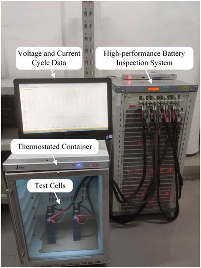
FIGURE 2. Experimental equipment for charging and discharging.

3.1 Construction of the XGB-AKF kalman filter

The Kalman filter algorithm mainly combines observations with prior state estimates to make optimal estimates of the system state through time updates and observation updates (Guo et al., 2019). The temporal update refers to Eq. 16–17, which substitute the optimal estimate of the system state at moment k-1, $x_{k-1}^{+}$ into the state equation to derive the a priori estimate $x_k^{-}$ at moment k. The observation update is accomplished by Eq. 19–20, combining the current observation $\left(z_k\right)$ and the a priori state estimate ${(x}_k^{-})$ to correct the system state ${(x}_k^{+})$.

To establish the Kalman filter equation for the XGB-KF model, the initial value of the system state is preferred to determine the initial value of the cell SOH as the state variable $\left(x_0^{+}\right)$.The initial ${SOH}_0^{+}$ is about 100% and the initial error covariance ${(P}_0^{+})$ is about 0 because the selected cell is brand new. The estimation accuracy of the joint estimation model mainly depends on the XGBoost model, and the Kalman filter mainly plays the role of correction filtering. Therefore, the measurement noise variance (R) should be set smaller than the system state noise variance (Q). To verify the effectiveness of the algorithm, several experiments were conducted, in which the typical data are as follows.

As shown in Figure 3, the current SOHs of the cell and the cycle times were closely related. Therefore, this paper uses the linear equation fitted with the average decreasing trend of SOH for cell1, cell 2, and cell 3 as the state equation; A_k = 1, and the slope of the straight line is K_avg.

FIGURE 3

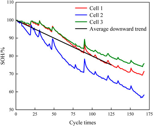
FIGURE 3. Training set with SOH and cycle number.

Due to the phenomenon that reactants may dissipate after standing for a period of time, the cell may exhibit capacity rebound, which has been found to be closely related to the rest time (Tang et al., 2014; Qin et al., 2017). In this paper, to improve the model prediction accuracy, the capacity rebound amount is added to the equation of state $U_k$, when the cell’s rest time is greater than the threshold. According to the relationship between the rest times and SOHs of cells 1, 2, and 3, there was a significant capacity rebound phenomenon at a rest time threshold of about 1 h, with an average rest capacity rebound $\left(C_{rest}\right)$ of 2%, as shown in Figures 4 and 5. Then the a priori state estimation equation is as follows:

$\begin{array}{c}{SOH}_k^{-}={SOH}_{k-1}^{+}+K_{avg}+U_k{C}_{rest}\end{array}(29)$

FIGURE 4

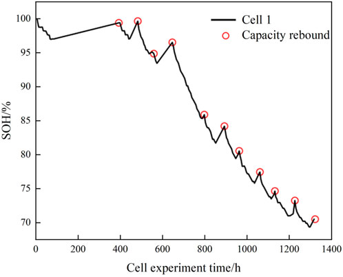
FIGURE 4. Cell one rest time greater than threshold cycle mark.

FIGURE 5

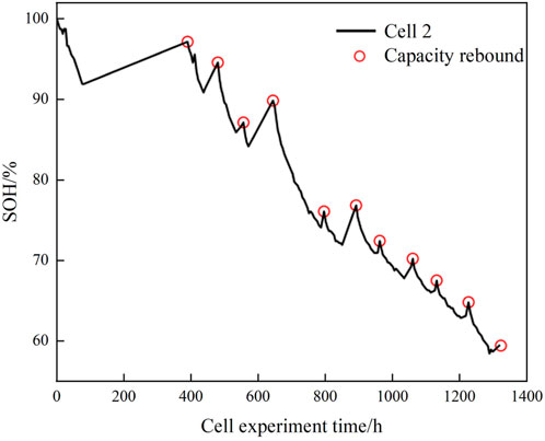
FIGURE 5. Cell two rest time greater than threshold cycle mark.

The SOH estimation output from the XGBoost online estimation model based on the kth cycle of the cell extracted features ($f_k$) is used as the observation $\left(z_k\right)$; then, $C_k$ = 1, and its system state update equation is as follows:

$\begin{array}{c}{SOH}_k^{+}={SOH}_k^{-}+K_k\left(XGB\left(f_k\right)-{SOH}_k^{-}\right)\end{array}(30)$

We determine the initial value of the system and update the equations back into the Kalman filter algorithm. When completing each charge/discharge cycle, the joint optimal estimation is achieved by the Kalman filter algorithm by weighing the estimated results of the observation equation XGBoost and the a priori estimation based on the time series.

3.2 Implementation of the joint XGB-AKF estimation method

After setting the initial values of the system state, they are substituted into the Kalman filter iteration formula to realize the real-time correction of the XGBoost estimation results. The Kalman filter algorithm substitutes the last cycle estimate ${(SOH}_{k-1}^{+})$ into Eq. 29 to derive the current cycle’s a priori estimated ${SOH}_k^{-}$. The state correction processcalculates the Kalman gain, substitutes the observed value into the state update Equation 30, weighs the observed value and the a priori estimate, corrects the current cycle cell health state ${(SOH}_k^{+})$, and updates the noise variance and error covariance to prepare for the next iteration.

The AKF corrects the error fluctuations of the XGBoost estimation results according to its state equations based on the determined initial state and the degradation trend of the rest time with cycle number. The adaptive noise algorithm is added to enhance the random noise adaptation and filter the disturbing noise in the data to make the final estimation results smoother and more accurate. The overall structural framework of the joint XGB-AKF estimation model is shown in Figure 6.

FIGURE 6

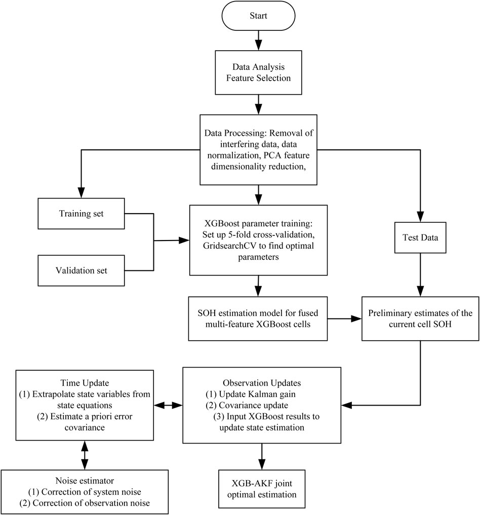
FIGURE 6. XGB-AKF model to estimate SOH framework for Li-ion cells.

3.3 Results validation and analysis

Cell four is used as a test battery to verify the accuracy of the model, and cells 1, 2, and three are used to complete the training of the XGBoost model. The characteristic data of the test cell after each cycle are extracted as the input of the XGBoost model. The preliminary SOH estimation results are then fed into the joint estimation model Kalman filter for correction filtering, and the final SOH joint estimation value of all cycles of cell4 is obtained. The estimation results based on the joint XGB-AKF estimation model, the XGBoost model, and the XGB-KF model without the adaptive filtering process are shown in Figures 7–9, respectively, and summarized in Table 1.

FIGURE 7

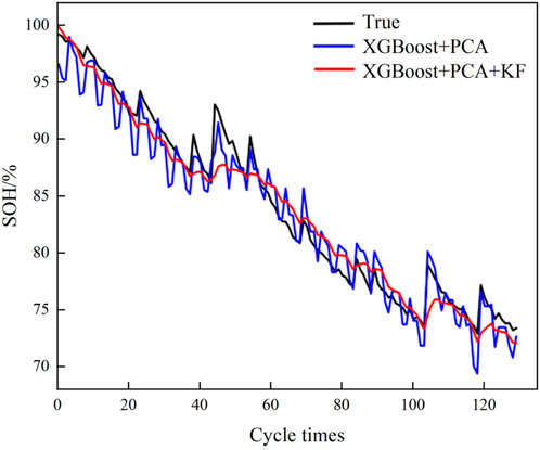
FIGURE 7. XGB-KF model to estimate SOH results for Li-ion cells.

FIGURE 8

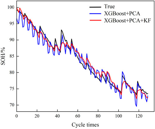
FIGURE 8. XGB-AKF model to estimate SOH results for Li-ion cells.

FIGURE 9

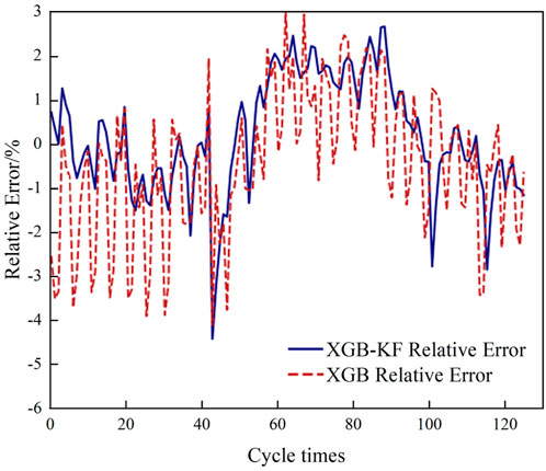
FIGURE 9. Comparison of the relative errors of XGB and XGB-KF model test sets.

TABLE 1

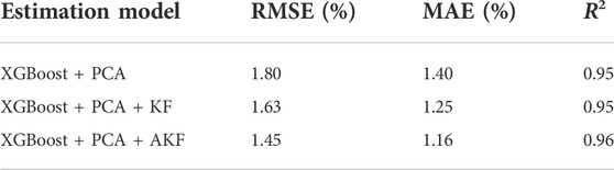
TABLE 1. Evaluation indicators based on joint model estimation results.

According to the evaluation metrics of different models in Table 2, the joint mean errors of the XGB-KF and XGB-AKF estimation models are found to be 10.7% and 17.1% lower than the XGBoost results, and the root-mean-square errors are reduced by 9.4% and 19.4%, respectively. The R² is above 0.95, indicating that all three algorithms fit well. Thus, the average error and root-mean-square error of the joint estimation model with the Kalman filter algorithm are reduced, and the average error between the estimated results and the true values is about 1.2%. The prediction curve is smoother and more accurate when the Kalman filter is introduced, which suppresses the error fluctuations caused by the XGBoost data-driven model influenced by historical data. The root mean square error and mean error of XGB-AKF (with the introduction of adaptive filtering) were reduced by 11.0% and 7.2% compared to XGB-KF, respectively. The larger decrease in the root mean square error indicates that the adaptive filtering mainly enhances the estimation adaptability and robustness of the joint estimation model.

TABLE 2

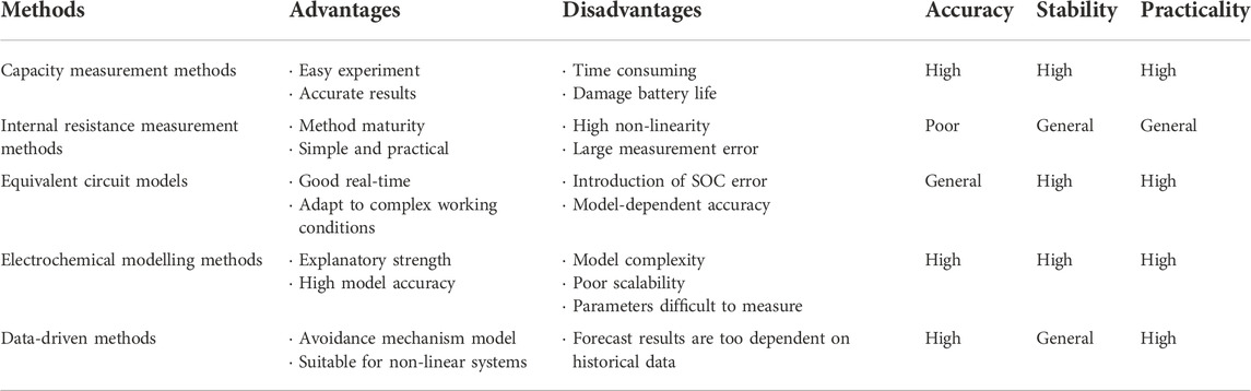
TABLE 2. Evaluation indicators based on joint model estimation results.

4 Conclusion

In this paper, the XGBoost data-driven model and the Kalman filter algorithm are combined to correct the fluctuation error of XGBoost by Kalman filtering the state equation based on the degradation trend of the time series. The joint XGB-AKF-based SOH estimation method for lithium-ion cells firstly constructs an online estimation model based on data-driven XGBoost. Then, the system is enhanced by introducing an adaptive Karman filtering algorithm with noise reduction filtering capability, and the XGBoost estimation results are corrected according to the time-domain equation of state. The results show that the method compensates for the shortcomings of the XGBoost data-driven algorithm—which is affected by the uncertainty of historical data and the Kalman filtering—and improves the accuracy and robustness of the estimation model to achieve a high-precision joint estimation of SOH for Li-ion cells.

Data availability statement

The original contributions presented in the study are included in the article/supplementary material, further inquiries can be directed to the corresponding author.

Author contributions

All authors listed have made a substantial, direct and intellectual contribution to the work, and approved it for publication.

Acknowledgments

The authors are grateful to the Science and Technology Project 5216A521001K of the State Grid Hunan Electric Power Company.

Conflict of interest

SX, F-LZ, B-WH, BY, H-BH, TZ, W-QM, J-JW, J-QW, S-KG, TW, X-YD, and S-FX are employed by the company Hunan Electric Power Co., Ltd.

Publisher’s note

All claims expressed in this article are solely those of the authors and do not necessarily represent those of their affiliated organizations, or those of the publisher, the editors and the reviewers. Any product that may be evaluated in this article, or claim that may be made by its manufacturer, is not guaranteed or endorsed by the publisher.

References

Abdi, H., and Williams, L. J. (2010). Principal component analysis. WIREs. Comp. Stat. 2, 433–459. doi:10.1002/wics.101

CrossRef Full Text | Google Scholar

Berecibar, M., Gandiaga, I., Villarreal, I., Omar, N., Van Mierlo, J., and Van den Bossche, P. (2016). Critical review of state of health estimation methods of Li-ion batteries for real applications. Renew. Sustain. Energy Rev. 56, 572–587. doi:10.1016/j.rser.2015.11.042

CrossRef Full Text | Google Scholar

Carkhuff, B. G., Demirev, P. A., and Srinivasan, R. (2018). Impedance-based battery management system for safety monitoring of lithium-ion batteries. Ieee Trans. Ind. Electron. 65, 6497–6504. doi:10.1109/TIE.2017.2786199

CrossRef Full Text | Google Scholar

Chai, J., Liu, Y., Wang, A., Qu, S., and Ouyang, Y. (2022). Prediction of strata behaviors law based on GRU and XGBoost. Gong-Kuang Zidonghua 48, 91–97. doi:10.13272/j.issn.1671-251x.2021070062

CrossRef Full Text | Google Scholar

Chang, C., Wang, Q., Jiang, J., and Wu, T. (2021). Lithium-ion battery state of health estimation using the incremental capacity and wavelet neural networks with genetic algorithm. J. Energy Storage 38, 102570. doi:10.1016/j.est.2021.102570

CrossRef Full Text | Google Scholar

Chen, F. E. I., Zhao, L., Wang, Y., and Wang, S. (2022). SOH estimation of Li-ion battery based on XGBoost algorithm. Zhejiang Dianli 41, 14–21. doi:10.19585/j.zjdl.202205003

CrossRef Full Text | Google Scholar

Chen, Z., and Wang, Q. (2014). “The application of UKF algorithm for 18650-type lithium battery SOH estimation,” in Computer and information technology. Editors P. Yarlagadda, S. B. Choi, and Y. H. Kim (Durnten-Zurich: Trans Tech Publications Ltd), 1079–1084. doi:10.4028/www.scientific.net/AMM.519-520.1079

CrossRef Full Text | Google Scholar

Garcia, R. V., Pardal, P. C. P. M., Kuga, H. K., and Zanardi, M. C. (2019). Nonlinear filtering for sequential spacecraft attitude estimation with real data: Cubature Kalman Filter, Unscented Kalman Filter and Extended Kalman Filter. Adv. Space Res. 63, 1038–1050. doi:10.1016/j.asr.2018.10.003

CrossRef Full Text | Google Scholar

Gholizadeh, M., and Yazdizadeh, A. (2020). Systematic mixed adaptive observer and EKF approach to estimate SOC and SOH of lithium-ion battery. IET Electr. Syst. Transp. 10, 135–143. doi:10.1049/iet-est.2019.0033

CrossRef Full Text | Google Scholar

Guo, F., Hu, G., Xiang, S., Zhou, P., Hong, R., and Xiong, N. (2019). A multi-scale parameter adaptive method for state of charge and parameter estimation of lithium-ion batteries using dual Kalman filters. Energy 178, 79–88. doi:10.1016/j.energy.2019.04.126

CrossRef Full Text | Google Scholar

Jain, P., Saha, S., and Sankaranarayanan, V. (2021). “Novel method to estimate SoH of lithium-ion batteries,” in 2021 Innovations in energy management and renewable resources(iemre 2021), Kolkata, India, 05-07 February 2021 (IEEE). doi:10.1109/IEMRE52042.2021.9386881

CrossRef Full Text | Google Scholar

Jing-tai, L., and Wang, X. (2022). XGBoost for imbalanced data based on cost-sensitive activation function. Ji Suan Ji Ke Xue 49, 135–143. doi:10.11896/jsjkx.210400064

CrossRef Full Text | Google Scholar

Klass, V., Behm, M., and Lindbergh, G. (2014). A support vector machine-based state-of-health estimation method for lithium-ion batteries under electric vehicle operation. J. Power Sources 270, 262–272. doi:10.1016/j.jpowsour.2014.07.116

CrossRef Full Text | Google Scholar

Lai, X., Wang, S., Ma, S., Xie, J., and Zheng, Y. (2020). Parameter sensitivity analysis and simplification of equivalent circuit model for the state of charge of lithium-ion batteries. Electrochimica Acta 330, 135239. doi:10.1016/j.electacta.2019.135239

CrossRef Full Text | Google Scholar

Li, H., Tan, Y., Dong, R., and Cheng, R. (2020). Modified Kalman filtering for Hammerstein systems with dynamic hysteresis. Kongzhi Lilun Yu Yingyong 37, 767. doi:10.7641/CTA.2019.90114

CrossRef Full Text | Google Scholar

Li, R., Li, W., Zhang, H., Zhou, Y., and Tian, W. (2021). On-line estimation method of lithium-ion battery health status based on PSO-svm. Front. Energy Res. 9, 693249. doi:10.3389/fenrg.2021.693249

CrossRef Full Text | Google Scholar

Liu, D., Pang, J., Zhou, J., Peng, Y., and Pecht, M. (2013). Prognostics for state of health estimation of lithium-ion batteries based on combination Gaussian process functional regression. Microelectron. Reliab. 53, 832–839. doi:10.1016/j.microrel.2013.03.010

CrossRef Full Text | Google Scholar

Long, B., Xian, W., Jiang, L., and Liu, Z. (2013). An improved autoregressive model by particle swarm optimization for prognostics of lithium-ion batteries. Microelectron. Reliab. 53, 821–831. doi:10.1016/j.microrel.2013.01.006

CrossRef Full Text | Google Scholar

Ma, L., and Cheng, S. (2022). Abnormal state early warning of Wind turbine generator based on support vector data description and XGBoost. Dian Gong Ji Shu Xue Bao 37, 3241. doi:10.19595/j.cnki.1000-6753.tces.210625

CrossRef Full Text | Google Scholar

Myers, K. A., and Tapley, B. D. (1976). Adaptive sequential estimation with unknown noise statistics. IEEE Trans. Autom. Contr. 21, 520–523. doi:10.1109/TAC.1976.1101260

CrossRef Full Text | Google Scholar

Oldham, K. B. (2008). A Gouy-Chapman-Stern model of the double layer at a (metal)/(ionic liquid) interface. J. Electroanal. Chem. (Lausanne). 613, 131–138. doi:10.1016/j.jelechem.2007.10.017

CrossRef Full Text | Google Scholar

Qin, T., Zeng, S., Guo, J., and Skaf, Z. (2017). State of health estimation of Li-ion batteries with regeneration Phenomena: A similar rest time-based prognostic framework. Symmetry (Basel). 9, 4. doi:10.3390/sym9010004

CrossRef Full Text | Google Scholar

Shi, G., Chen, S., Yuan, H., You, H., Wang, X., Dai, H., et al. (2021). Determination of optimal indicators based on statistical analysis for the state of health estimation of a lithium-ion battery. Front. Energy Res. 9, 690266. doi:10.3389/fenrg.2021.690266

CrossRef Full Text | Google Scholar

Sinopoli, B., Schenato, L., Franceschetti, M., Poolla, K., Jordan, M. I., and Sastry, S. S. (2004). Kalman filtering with intermittent observations. IEEE Trans. Autom. Contr. 49, 1453–1464. doi:10.1109/TAC.2004.834121

CrossRef Full Text | Google Scholar

Tan, X., Liu, X., Wang, H., Fan, Y., and Feng, G. (2022). Intelligent online health estimation for lithium-ion batteries based on a parallel attention network combining multivariate time series. Front. Energy Res. 10, 844985. doi:10.3389/fenrg.2022.844985

CrossRef Full Text | Google Scholar

Tang, S., Yu, C., Wang, X., Guo, X., and Si, X. (2014). Remaining useful life prediction of lithium-ion batteries based on the wiener process with measurement error. Energies 7, 520–547. doi:10.3390/en7020520

CrossRef Full Text | Google Scholar

Waag, W., Kaebitz, S., and Sauer, D. U. (2013). Experimental investigation of the lithium-ion battery impedance characteristic at various conditions and aging states and its influence on the application. Appl. Energy 102, 885–897. doi:10.1016/j.apenergy.2012.09.030

CrossRef Full Text | Google Scholar

Widodo, A., and Yang, B.-S. (2011). Machine health prognostics using survival probability and support vector machine. Expert Syst. Appl. 38, 8430–8437. doi:10.1016/j.eswa.2011.01.038

CrossRef Full Text | Google Scholar

Wu, J., Mei, F., Zheng, J., Zhang, Z., and Zuo, H. (2022). Classification of power quality composite disturbances based on improved empirical wavelet transform and XGBoost. Dian Gong Ji Shu Xue Bao 37, 232. doi:10.1049/gtd2.12407

CrossRef Full Text | Google Scholar

Xiong, R., Li, L., and Tian, J. (2018). Towards a smarter battery management system: A critical review on battery state of health monitoring methods. J. Power Sources 405, 18–29. doi:10.1016/j.jpowsour.2018.10.019

CrossRef Full Text | Google Scholar

Yan, D. (2016). Spatial kalman filtering and spatial-temporal kalman filtering algorithm. Lanzhou Li Gong Xue Xue Bao J. Lanzhou Univ. Technol. Lanzhou Ligong Daxue Xuebao 42, 5323. doi:10.1109/ICOSP.2014.7015323

CrossRef Full Text | Google Scholar

Yang, N., Yu, T., Luo, Q., and Wang, K. (2022). Fast and accurate health assessment of lithium-ion batteries based on typical voltage Segments. Front. Energy Res. 10, 925947. doi:10.3389/fenrg.2022.925947

CrossRef Full Text | Google Scholar

Zhang, D., Zhao, W., Wang, L., Chang, X., Li, X., and Wu, P. (2022). Evaluation of the state of health of lithium-ion battery based on the temporal convolution network. Front. Energy Res. 10, 929235. doi:10.3389/fenrg.2022.929235

CrossRef Full Text | Google Scholar

Zhu, W., and He, F. (2019). Adaptive kalman filtering based on variable weight innovation covariance. Xi Hua Xue Xue Bao J. Xihua Univ. Zi Ran Ke Xue Ban. 33, 23 doi:10.3969/j.issn.1001-506X.2011.12.23

CrossRef Full Text | Google Scholar