An improved deep learning algorithm in enabling load data classification for power system

Load behaviors significantly impact the planning, dispatching, and operation of the modern power systems. Load classification has been proved as one of the most effective ways of analyzing the load behaviors. However, due to the issues of data collection, transmission, and storage in current power systems, data missing problems frequently occur, which prevents the load classification tasks from precisely identifying the load classes. Simultaneously, because of the diversities of the load categories, different loads contribute various amounts of data, which causes the class imbalance issue. The traditional load data classification algorithms lack the ability to solve the aforementioned issues, which may deteriorate the load classification accuracy. Therefore, this study proposed an improved deep learning algorithm based on the load classification approach in terms of raising the classification performances with solving the data missing and class imbalance issues. First, the LATC (low-rank autoregressive tensor completion) algorithm is used to solve the data missing issue to improve the quality of the training dataset. A Borderline-SMOTE algorithm is further adopted to improve the class distribution in the training dataset to improve the training performances of biGRU (bidirectional gated recurrent unit). Afterward, to improve the classification accuracy in the classification task, the biGRU algorithm, combined with the attention mechanism, is used as the underlying infrastructure. The experimental results show the effectiveness of the proposed approach.

1 Introduction

It is admitted that loads could significantly influence the planning, dispatching, and operation of the modern power systems (Xu et al., 2017; Liu et al., 2020; Liu et al., 2021; Ullah et al., 2022). Hongbo et al. (2019) and Hong and Hsiao (2022) pointed out that the load is one of the most important factors that determine the locations and the capacities of generators in power system planning. Jia et al. (2019) and Yao et al. (2019) suggested that loads are also a key factor of modern power system economic dispatch. Ross and Mathieu (2021) and Harishma et al. (2022) demonstrated that power system safe operation also depends on load characteristics. Therefore, although challenging, it is important to figure out an effective way of analyzing load in the power system field. Currently, the load classification has been proven as the most suitable method for obtaining load awareness (Yang et al., 2018; Alam et al., 2020; Phyo and Jeenanunta, 2021).

Traditionally, researchers mainly focused on the unsupervised machine learning algorithms, such as K-means (Sinaga and Yang, 2020), FCM (fuzzy C-means) (Sun et al., 2019a), and DBSCAN (density-based spatial clustering of applications with noise) (Aref et al., 2020) algorithms. Peng et al. (2014) identified the patterns of the power load using K-means, K-medoids, SOM (self-organizing maps), and FCM. Based on the experimental results, the authors verified the effectiveness of these algorithms. Hu et al. (2018) optimized the initial centroids using the density parameters to overcome the disadvantages of K-means in load classification and successfully improved the performance of K-means. Xu et al. (2015) presented a clustering hierarchy process based on the kernel fuzzy C-means algorithm. Their approach also showed effectiveness in classification tasks. However, many works have pointed out that the aforementioned machine learning algorithms are extremely sensitive to the distribution of data instances in the dataset, which may deteriorate the load classification performances (Saravanan and Sujatha, 2018; Lin et al., 2019; Tian and Compere, 2019; Zhang et al., 2020a; Gramajo et al., 2020).

Therefore, supervised learning classification algorithms, such as SVM (support vector machine) (Dongsong and Qi, 2017), Bayesian network (Wang and Wang, 2005), and ANNs (approximate nearest neighbors) (Guo and Zhu, 2019), are developed and widely used in the classification problems. To achieve high accuracy of classifying user load profiles, Cai et al. (2017) improved the SVM algorithm by using the GMM (Gaussian mixture model). Wang and Wang (2005) combined the wavelet decomposition with the Bayesian network to classify the power quality disturbances. Wang et al. (2020) used zero-mean, batch-normalization, and rectified linear unit (ReLU) to optimize the input layer and hidden layers of BPNN (back propagation neural network) to improve the training of the BPNN. However, it has been pointed out by Niu et al. (2005); Yang et al. (2016); and Sun et al. (2019b) that these algorithms still encounter the prominent issues of low efficiency and overfitting, especially with the increasing load data dimension and the load data volume.

In this case, deep learning algorithms, such as RNN (recurrent neural network), have been adopted by researchers to analyze the high-dimensional load data (Greff et al., 2017; Lee et al., 2020). However, it is difficult for original RNNs to tackle the gradient disappearance and the long-term dependency issues. Therefore, Oslebo et al. (2019) presented the LSTM (long short–term memory) algorithm by adding the cell states into RNNs. Nonetheless, the LSTM algorithm could be affected by a large number of parameters, which finally results in overfitting (Pan et al., 2020; Sajjad et al., 2020). For this purpose, Le et al. (2016) further presented the GRU algorithm, which could effectively reduce the number of intrinsic parameters and thereby reduce the risk of over-fitting based on the simpler model. Moreover, the biGRU algorithm is proposed by Almuzaini and Azmi (2020) to make full use of the past and future data and this algorithm is further combined with the attention mechanism to highlight the important data characteristics. The authors demonstrated the ability of the proposed algorithm in terms of improving the classification efficiency and accuracy.

It is emphasized that the performance of the classification algorithm intensively depends on the data quality of the training dataset (Deng et al., 2019; Li et al., 2020). However, considering the complex and vulnerable process of data collection, transition, and storage, incomplete data situations due to data loss are inevitable and could even occur frequently (Park et al., 2020), which would certainly impact the quality of the training dataset. Therefore, the classification accuracy may benefit from improving the data integrity of the training dataset (Du et al., 2020). Currently, data completion algorithms, such as interpolation methods (Hosseini and Sebt, 2017; Yu et al., 2020; Zhang et al., 2021), KNN (K-nearest neighbor) completion algorithm (Marchang and Tripathi, 2021), and tensor completion algorithm (Yuan et al., 2018) (Su et al., 2019), have been widely adopted for maintaining and recovering the data integrity. Azarkhail and Woytowitz (2013) and Chu (2011) mentioned that the widely utilized data completion methods, such as the interpolation completion, can effectively complete the missing data. However, those algorithms are unable to handle the dataset with sequential features. Zhu et al. (2011) presented a data completion method based on the machine learning. Although the algorithm performs with good accuracy, it is difficult to obtain the complete data sequence. Chen and Sun (2020) presented the tensor completion algorithm, which can effectively reduce data completion errors and process time series data. This algorithm can be a suitable underlying infrastructure to compensate the dataset and improve the load classification accuracy.

Recently, a group of researchers pointed out that another data quality issue, namely, the class imbalance issue, should be carefully handled (Jing et al., 2017; Ebenuwa et al., 2019). This issue could also severely impact the training performance of machine learning algorithms. The imbalanced majority classes may overwhelm the minority classes, which leads to the insufficient training of the classification algorithm, and finally leads to low classification accuracy. In this case, Jeon and Lim (2020) adopted the undersampling method to solve the class imbalance issue. However, the method may mistakenly remove important sample information. Polat (2019) proposed the SMOTE (Synthetic Minority Over-sampling Technique) algorithm to overcome this issue of the undersampling method, but in addition, the occurrence possibility of overlap between classes and futile samples increases. Ghorbani and Ghousi (2020) further adopted the SMOTE algorithm by strengthening the border between the majority and minority classes. Their Borderline-SMOTE algorithm is able to create new samples at the borderline so that the majority and minority classes have higher chances to be distinguished in the training phase.

Currently, some researchers (Wang et al., 2019; Dogo et al., 2020; Dharmasaputro et al., 2022; Lepolesa et al., 2022) hybridized the three methods to implement the classification with data integrity and class imbalance issues. Lepolesa et al. (2022) addressed dataset weaknesses such as missing data and class imbalance problems through data interpolation and synthetic data generation processes. Dharmasaputro et al. (2022) proposed a preprocessing process to combine multiple imputation by chained equations (MICE) and SMOTE and tested it with three machine learning methods. Dogo et al. (2020) studied the methods including seven missing data and eight resampling methods, on 10 different learning classifiers. However, the algorithms adopted in those research studies have a certain defect which the studies mentioned before.

Therefore, this study proposed an improved deep learning method to raise classification performances. The LATC algorithm is used to complete the missing data and improve the quality of the training dataset. Different from the other data completion algorithms, it can achieve low-error data completion. Thereafter, the Borderline-SMOTE algorithm is adopted to resolve the class imbalance issue in the training dataset, especially tackling the instances at the borderline. At last, the attention mechanism integrated the biGRU algorithm is adopted to improve the classification accuracy. Based on the experimental results, the proposed improved deep learning method shows remarkable performance and effectiveness for the load classification tasks with the load data and with the data integrity and class imbalance issues.

The rest of the study is organized as follows: Section 2 proposes the details of the methodologies for the deep learning method improvements; Section 3 shows the experimental results; Section 4 concludes the study.

2 An improved biGRU based on LATC and Borderline-SMOTE algorithms

An incomplete dataset with time series representing electric power consumption is donated as $T^{M\times D\times n}$, where M represents the member, D represents the number of days, and n represents the test time for load in a day. The dataset has the class imbalance issue. This section introduces the LATC algorithm which solves the data missing issue and details the Borderline-SMOTE algorithm that can improve the class distribution in the dataset. Afterward, we introduced the attention mechanism–integrated biGRU algorithm. The process of the proposed algorithm is shown at last.

2.1 Low-rank autoregressive tensor completion

The tensor is a high-dimensional array. Its dimension is usually referred as order. For an incomplete tensor $\mathcal{Y}\in {\mathbb{R}}^{l_1\times l_2\times \cdots \times l_N}$, $l_n$ represents the nth dimension. Furthermore, as the extended form of the matrix, the tensor can possess the low-rank characteristic of the matrix (Yuan et al., 2018). Thus, the low-rank tensor completion (LRTC) algorithm is able to utilize the aforementioned characteristic to obtain the different low-rank structure of the time series data, which indicates the characteristic of users’ load. Therefore, $\mathcal{Y}$ can be completed as the recovered tensor $\mathcal{X}$ by solving the following optimization problem.

$\begin{array}{c}\underset{\mathcal{X}}{\min }rank\left(\mathcal{X}\right)\\ s.t.P_{\Omega }\left(\mathcal{X}\right)=P_{\Omega }\left(\mathcal{Y}\right),\end{array}(1)$

where $P_{\Omega }$ represents an orthogonal projection operator onto the observed set Ω such as

$P_{\Omega }{\left(\mathcal{X}\right)}_{i,j}=\{\begin{array}{c}{x}_{i,j},if\left(i,j\right)\in \Omega \\ 0,otherwise.\end{array}(2)$

However, the problem Eq. 1 is generally NP-hard (Chen and Sun, 2020) due to the non-convex and potentially discontinuous nature of the rank function. The optimization problem can be reformulated as Eq. 3 by using the nuclear norm (NN):

$\begin{array}{c}\underset{\mathcal{X}}{\min }{\Vert \mathcal{X}\Vert }_{\ast }\\ s.t.P_{\Omega }\left(\mathcal{X}\right)=P_{\Omega }\left(\mathcal{Y}\right).\end{array}(3)$

The NN is defined as ${\Vert \mathcal{X}\Vert }_{\ast }={\displaystyle \sum }_k{\sigma }_k{\Vert {\mathcal{X}}_{\left(k\right)}\Vert }_{\ast }$, where ${\sigma }_k$ is a non-negative weight parameter with ${\displaystyle \sum }_k{\sigma }_k=1$. ${\mathcal{X}}_{\left(k\right)}$ represents the kth-mode unfolding of $\mathcal{X}$.

However, a time series load data collected before preprocessing is usually expressed as a second-order matrix. Therefore, the incomplete matrix of the time series load data $\mathit{Y}\in {\mathbb{R}}^{M\times \left(IJ\right)}$ can be covered into tensor $\mathcal{S}\left(\mathit{Y}\right)\in {\mathbb{R}}^{M\times I\times J}$. The operator $\mathcal{S}\left(.\right)$ converts the multivariate time series matrix into a third-order tensor. Correspondingly, ${\mathcal{S}}^{-1}\left(.\right)$ denotes the inverse operator that converts the third-order tensor into a multivariate time series matrix.

Moreover, the time series load data can be more randomized (Chen and Sun, 2020) than other data, which means the missing data $I_j$ are closely related to $I_{j-1}$ and $I_{j+1}$. For this purpose, the autoregressive norm (Chen and Sun, 2020) is used to effectively model the short-term or local trends. The autoregressive norm of matrix Z with a lag set H and coefficient matrix A is defined as Eq. 4.

${\Vert \mathit{Z}\Vert }_{\mathit{A},H}={\sum }_{m,t}{\left(z_{m,t}-{\displaystyle \sum }_i{a}_{m,i}{z}_{m,t-h_i}\right)}^2,(4)$

where $h_i\in H=\left\{h_1,\cdots ,h_d\right\}$ represents a time lag, and $\mathit{Z}\in {\mathit{R}}^{M\times \left(IJ\right)}$.

Therefore, the optimization problem of the low-rank autoregressive tensor completion (LATC) algorithm can be defined as

$\underset{\mathcal{X},\mathit{Z},\mathit{A}}{min}{\Vert \mathcal{X}\Vert }_{\ast }+\lambda {\Vert \mathit{Z}\Vert }_{\mathit{A},H,}(5)$

$s.t.\{\begin{array}{c}X=S\left(\mathit{Z}\right),\\ P_{\Omega }\left(\mathit{Z}\right)=P_{\Omega }\left(\mathit{Y}\right),\end{array}(6)$

where $\mathcal{X}$ represents the recovered tensor. $\lambda$ represents a weight parameter that balances the trade-off between the two terms in the objective function.

In order to simplify the evaluation of the coefficient matrix A, the independent autoregressive model is used. In addition, auxiliary variables ${\mathcal{X}}_k$ are introduced to solve the optimization problem.

$\underset{{\left\{{\mathcal{X}}_k\right\}}_{k=1}^3,\mathit{Z},\mathit{A}}{\min }{\sum }_k{\alpha }_k{\Vert {\mathcal{X}}_{k\left(k\right)}\Vert }_{\ast }+\lambda {\Vert \mathit{Z}\Vert }_{\mathit{A},H},(7)$

$\mathrm{s}.\mathrm{t}.\{\begin{array}{c}{\mathcal{X}}_k=S\left(\mathit{Z}\right),k=\mathrm{1,2,3},\\ P_{\Omega }\left(\mathit{Z}\right)=P_{\Omega }\left(\mathit{Y}\right),\end{array}(8)$

where ${\mathcal{X}}_{k\left(k\right)}$ represents the kth-mode unfolding of ${\mathcal{X}}_k$.

Furthermore, the parameter iteration process can be derived from the alternating direction method of multiplier (ADMM) framework and the three lemmas in Chen and Sun (2020).

${\mathcal{X}}_k^{l+1}:=fol{d}_k\left({\mathcal{D}}_{\frac{{\alpha }_k}{\rho }}\left(\mathcal{S}{\left({\mathit{Z}}^l\right)}_{\left(k\right)}-{\mathcal{T}}_{k\left(k\right)}^l/\rho \right)\right),(9)$

${\mathit{Z}}_{\left[:h_d\right]}^{l+1}:=\frac{1}{3}{\sum }_k{\mathcal{S}}^{-1}{\left({\mathcal{X}}_k^{l+1}+{\mathcal{T}}_k^l/\rho \right)}_{\left[:h_d\right]},(10)$

$z_{m,\left[h_d+1:\right]}^{l+1}:=\frac{1}{3\left(\rho +\lambda \right)}{\sum }_k{\mathcal{S}}^{-1}{\left(\rho {\mathcal{X}}_k^{l+1}+{\mathcal{T}}_k^l\right)}_{m,\left[h_d+1:\right]}+\frac{\lambda }{\rho +\lambda }{\mathit{Q}}_m{\alpha }_m^l,(11)$

${\alpha }_m^{l+1}:={\mathit{Q}}_m^{+}{z}_{m,\left[h_d+1:\right]}^{l+1},(12)$

${\mathcal{T}}^{l+1}:={\mathcal{T}}^l+\rho \left({\mathcal{X}}_k^{l+1}-\mathcal{S}\left({\mathit{Z}}^{l+1}\right)\right).(13)$

Ultimately, the recovered tensor $\mathcal{X}$ can be obtained.

2.2 Borderline-SMOTE algorithm

The Borderline-SMOTE (Chen et al., 2021) algorithm, which is developed from SMOTE, divides the minority samples into three classes: safe, danger, and noise classes. If there are more than half minority samples surrounding the target sample, the target sample is indicated as a safe sample. If there are more than half majority samples surrounding the target sample, the target sample is indicated as a dangerous sample. If the samples surrounding the target sample are all majority samples, the target sample is indicated as a noise sample. In order to avoid the aliasing phenomenon existing in SMOTE, only danger samples can be further processed. The process of the Borderline-SMOTE algorithm is as follows:

1) In the training dataset T, for each sample $p_i\left(i=\mathrm{1,2},\cdots ,p_{num}\right)$ in the minority class P, calculate a set of $m$ nearest neighbors. From the nearest neighbors, the number of majority samples is $m^{\prime }\left(0\le m^{\prime }\le m\right)$

2) If $p_i$ belongs to the safe samples, $p_i$ need not to be further processed. If $p_i$ belongs to the danger samples, $p_i$ need to have the step 3). If $p_i$ belongs to the noise sample, $p_i$ has to be neglected.

3) For each borderline sample $p_i^{\prime }\in \mathrm{B}$, calculate the number of k nearest neighbors from the minority class P, and then a number of s points are randomly selected from the k neighbors to have linear interpolation with $p_i^{\prime }$. As a result, a new instance synthetic $p_j=p_i^{\prime }+r_j\cdot \left(p_i^{\prime }-p_j^{\prime }\right)$ can be ultimately synthesized. $r_j$ denotes a random value between 0 and 1.

The algorithm is able to create new instances to tackle the class imbalance issue as well as to identify the border between two classes. However, it should be also noted that the parameter k affects the performance of the Borderline-SMOTE algorithm. Therefore, the optimal value of k is selected from a series of pretreatment experiments in the later algorithm evaluation parts.

2.3 Attention mechanism–integrated biGRU algorithm

High-dimensional load data could reduce the classification accuracy (Wang and Wang, 2005; Cai et al., 2017; Guo and Zhu, 2019). It has been shown that the GRU algorithm outperforms in handling high-dimensional data compared with algorithms such as traditional LSTM (Pan et al., 2020; Sajjad et al., 2020), and additionally can reduce the number of parameters. Therefore, this study used biGRU as the underlying algorithm to conduct the classification task. In addition, the attention mechanism is also integrated to highlight the important features of the load data.

2.3.1 GRU algorithm and biGRU algorithm

The GRU (gated recurrent unit) algorithm is proposed based on the LSTM algorithm (Zhang et al., 2020b). It significantly simplifies the cell structure by aggregating the forgotten gate and the input gate into an update gate, which observably leads to the reduction of the parameters. Therefore, the GRU algorithm has a great potential of outperforming LSTM in terms of efficiency and accuracy. The internal structure of the GRU algorithm is shown in Figure 1.

$z_t=\sigma \left(W_z\cdot \left[h_{t-1},x_t\right]\right),(14)$

$r_t=\sigma \left(W_r\cdot \left[h_{t-1},x_t\right]\right),(15)$

$\stackrel{\sim }{h_t}=\tanh \left(W\cdot \left[r_t\ast h_{t-1},x_t\right]\right),(16)$

$h_t=\left(1-z_t\right)\ast h_{t-1}+z_t\ast \stackrel{\sim }{h_t,}(17)$

where $z_t,r_t,\stackrel{\sim }{h_t},h_t$ represent the update gate, reset gate, new memory, and hidden state, respectively. The hidden layer is consisted of the new memory and the hidden state. $x_t$ represents the input in time t. Also, $W_z,W_r,W$ represent the weight matrixes.

FIGURE 1

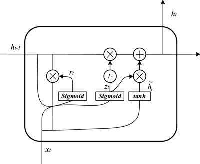
FIGURE 1. Internal structure of the GRU unit.

Normally, a GRU layer in a deep learning model consists of GRUs to accomplish the classification tasks. It should be noted that the GRU layer can process the time series data in one direction. However, the time series data at time t are related to the time series data at t-1 and t+1 from both directions. The biGRU model, which consists of the forward GRU and the backward GRU, can handle the aforementioned problem. It can potentially provide a high-accuracy classification method. The structure of the biGRU model is shown in Figure 2.

FIGURE 2

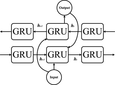
FIGURE 2. Structure of the biGRU model.

2.3.2 Attention mechanism

The attention mechanism especially concentrates on the available information for specific tasks. The attention assigns different values to different features of the time series, which can filter and highlight the most important features from the original features of a training dataset. The process of the attention mechanism is introduced as follows:

1) One array of the time series data in a training dataset can be represented as $\mathit{X}=\left(x_1,x_2,\cdots ,x_n\right)$ for the input of the attention mechanism. Each $x_i$ can be regarded as a <key, value > pair, where key represents the address of the time series data; and value represents the value of the time series data. In addition, the attention value can be described as the mapping of the <key, value> about the query, where query represents the hidden status of time t.

2) The matrix of Q (K, V) can be obtained by multiplying the X and $W^Q$ ($W^K$, $W^V$), which can be acquired by training with the dataset.

$\begin{array}{l}Q=\left(q_1{,q}_2,\cdots {,q}_i\right),\\ K=\left(k_1{,k}_2,\cdots {,k}_i\right),\\ V=\left(v_1{,v}_2,\cdots {,v}_i\right).\end{array}(18)$

3) The correlation value between query and key can be calculated.

4) The $\sqrt{d}$ is divided in order to avoid the overlarge result, which is the number of the hidden size.

5) The final attention value can be obtained by multiplying the matrix V and the SoftMax function that is used to normalize the weight coefficient of each key corresponding to the value. The attention value can be eventually expressed as in Eq. 19.

$Attentio{n}_{Q,K,V}=softmax\left(\frac{Q{K}^T}{\sqrt{d}}\right)V.(19)$

2.4 An improved deep learning algorithm

Traditional classification methods generally lack the ability to handle the missing and imbalanced dataset. Therefore, LATC and Borderline-SMOTE algorithms are used to enhance the classification accuracy of the proposed deep learning algorithm.

Being a supervised learning classification algorithm, the biGRU algorithm requires a training dataset with labels to conduct the training process. The LATC algorithm is adopted for the sake of completing the missing data to improving the quality of the training dataset. Moreover, because the random selection may aggravate the imbalance issue, the Borderline-SMOTE algorithm is further used to solve the class imbalance problem in the training dataset after the data missing issue has been addressed. At last, the attention mechanism–integrated biGRU algorithm is used to classify the training dataset. The training procedure is shown as in Figure 3.

FIGURE 3

FIGURE 3. Classification model training process.

A raw dataset usually contains invalid information for classification. Therefore, the data preprocessing is conducted first to exclude the invalid information and the load dataset $T^{M\times D\times n}$ can be obtained. The load dataset $T^{M\times D\times n}$ is reshaped as in Eq. 20.

$T^{M\times D\times n}=T^{\left(M\times D\right)\times n}=T^{ITEM\times n}=\left[\begin{array}{ccc}{I}_{11}& \cdots & I_{1n}\\ ⋮& \ddots & ⋮\\ I_{ITEM1}& \cdots & I_{ITEMn}\end{array}\right],(20)$

where $I_{ITEMn}$ means the ITEM^th electric power consumption of the dataset $T^{ITEM\times n}$ at the nth time point. However, the load data in $T^{ITEM\times n}$ do not have labels, which means it cannot be directly used with any supervised algorithm to train the classification model. Therefore, a K-means algorithm–based approach to label the original load data is proposed first. A number of samples are randomly selected from the original dataset and then the K-means algorithm is applied to process these samples. The preset number of clusters will influence the training performance. In this case, silhouette coefficient, inertia score, and Calinski Harabasz score are adopted to find out the optimal number of clusters.

Silhouette coefficient:

$S\left(i\right)=\frac{b\left(i\right)-a\left(i\right)}{\max \left(a\left(i\right),b\left(i\right)\right)},(21)$

where $a\left(i\right)$ that represents the average distance between i and other samples in the same category reflects the density of clusters. $b\left(i\right)$ that represents the average distance between i and other samples in the different category reflects the dispersibility of clusters. If $S\left(i\right)$ is closer to 1, the cluster results are more rational.

Inertia score:

$SSE={\sum }_{i=1}^k{\sum }_{p\in C_i}{\left|p-m_i\right|}^2,(22)$

where $C_i$ is the ith cluster, $p$ is the sample in $C_i$, $m_i$ is the centroid of $C_i$, and SSE is the clustering error of all samples.

Calinski Harabasz score:

$CH\left(k\right)=\frac{trB\left(k\right)/\left(k-1\right)}{trW\left(k\right)/\left(n-k\right)},(23)$

$B\left(k\right)={\sum }_q{n}_q\left(c_q-c\right){\left(c_q-c\right)}^T,(24)$

$W\left(k\right)={\sum }_{q=1}^k{\sum }_{x\in C_q}\left(x-c_q\right){\left(x-c_q\right)}^T,(25)$

where n represents the number of clustering samples, k represents the current cluster, $tr$ represents the trace of matrix, $c_q$ represents the core point of the q cluster, $C_q$ represents the rendezvous point, and $n_q$ represents the center. $B\left(k\right)$ is the covariance between categories and $W\left(k\right)$ is the covariance matrix within categories. The larger CH value means strong connections within a class and week connection between classes, and thereby indicates a better clustering result.

Based on the optimally clustering number of k, the sample data can be clustered into several clusters. Also then, in each cluster, we select a number of points which are close to the centroid as the training data $T_{train}{}^{item\times n}$ with labels $T_{label}{}^{item\times 1}$. The selection is based on the Euclidean distance as the following equation:

$dis\left(p_i,p_j\right)<\delta ,(26)$

where $dis\left(p_i,p_j\right)$ represents the Euclidean distance between $p_i$ and $p_j$, and $\delta$ represents the threshold value of the distance.

Furthermore, it is common that at some time points, some users are collecting their power consumption data, while others are not. This causes the load data of the users that are not collecting their power consumption data to be filled with 0, which is similar to occurrence of data missing. Therefore, it is essential to inspect whether data $I_j$ belong to the data missing issue via Eq. 27.

$\{\begin{array}{c}{I}_{j-1,j+1}\ne 0\\ I_j=0\end{array},j=\mathrm{2,3},\cdots ,n-1.(27)$

After a series of processes mentioned before, $T_{train}$ is able to be completed via the LATC algorithm. $\mathit{Y}=T_{train}$ and $\mathcal{X}=T_{train}{}^{item\times n}$ are applied in Algorithm 1 to solve the class imbalance problem. ${\alpha }_k$s represents non-negative weight parameters with ${\displaystyle \sum }_k{\alpha }_k=1$. $\rho$ represents the learning rate of the ADMM algorithm. $\lambda$ represents a weight parameter that balances the trade-off between the two terms in the objective function. $\theta$ represents a non-negative integer.

ALGORITHM 1

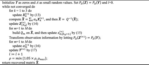
Algorithm 1. LATC algorithm.

It can be assumed that $T_{train}^{item\times n}$ has k clusters and the number of samples in different categories, respectively, are $n_1,n_2,\cdots ,n_{k-1},n_k$.

$T_{train}{}^{item\times n}=\left[\begin{array}{ccc}{I}_{11}& \cdots & I_{1n}\\ ⋮& \ddots & ⋮\\ I_{item1}& \cdots & I_{itemn}\end{array}\right],(28)$

After tackling the data integrity issue, $T_{train}{}^{item\times n}$ only having the class imbalance issue needs to be processed. Thus, the sample rate is $\sigma =\frac{n_j}{n_k}\left(j=\mathrm{1,2},\cdots ,k\right)$, $n_1^{\prime },n_2^{\prime },\cdots ,n_{k-1}^{\prime },n_k^{\prime }$ is the number of new samples in different categories by adopting the Borderline-SMOTE algorithm, $T_{label}{}^{ite{m}^{\prime }\times 1}$ is a set of new labels, and $T_{train}{}^{ite{m}^{\prime }\times n}$ is the training dataset after balancing. If $0<\sigma <{\sigma }_{\mathit{max}}$, then the minority samples, $n_j$ should be taken into the Borderline-SMOTE algorithm to get $n_1^{\prime },n_2^{\prime },\cdots ,n_{k-1}^{\prime },n_k^{\prime }$, $T_{label}{}^{ite{m}^{\prime }\times 1}$ and $T_{train}{}^{ite{m}^{\prime }\times n}$.

$T_{train}{}^{ite{m}^{\prime }\times n}=\left[\begin{array}{ccc}{I}_{11}& \cdots & I_{1n}\\ ⋮& \ddots & ⋮\\ I_{item1}& \cdots & I_{itemn}\\ I_{\left(ite{m}^{\prime }-item+1\right)1}\prime & \cdots & I_{\left(ite{m}^{\prime }-item+1\right)n}\prime \\ ⋮& \ddots & ⋮\\ I_{ite{m}^{\prime }1}^{\prime }& \cdots & I_{ite{m}^{\prime }n}^{\prime }\end{array}\right].(29)$

The deep learning method is utilized to classify the dataset $T_{train}{}^{ite{m}^{\prime }\times n}$ after being processed with LATC and Borderline-SMOTE algorithms. In order to enhance the classification accuracy and precision, the attention mechanism–integrated biGRU algorithm is adopted to highlight the necessary features in the time series. The architecture of the proposed deep learning algorithm is shown in Figure 4.

FIGURE 4

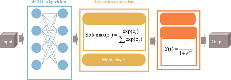
FIGURE 4. Architecture of the proposed deep learning algorithm.

From Figure 4, it can be seen that the training dataset is sequentially processed by the biGRU algorithm and the attention mechanism. Therefore, in order to fully consider the information in the forward and backward directions, Eq. 30 is adopted. In addition, the attention mechanism is considered to consist of a dense layer and a merge layer. The softmax function (Almuzaini and Azmi, 2020) is utilized to compute the reliability $z_i$ for the $i^{th}$ class as shown in Eq. 31. The load data need to be further processed in the output layer after the two steps. However, it is common that the load data classification is a multi-label task. Therefore, the sigmoid activation function is used as shown in Eq. 32.

$h{}_i=h_i^F\oplus h_i^B,(30)$

$Softmax\left(z_i\right)=\frac{exp\left(z_i\right)}{{\displaystyle \sum }_i\left(z_i\right)},(31)$

$S\left(t\right)=\frac{1}{1+e^{-t}},(32)$

where $h_i^F$ represents the forward sequence, and $h_i^B$ represents the backward sequence.

After the proposed deep learning algorithm processing, the samples in different categories $n_1^{″},n_2^{″},\cdots ,n_{k-1}^{″},n_k^{″}$ and a set of new labels ${T_{label}^{\prime }}^{ite{m}^{\prime }\times 1}$ can be obtained. The indexes, such as precision, recall rate, and f1-score, are used to evaluate the classification result. The classification determination indexes employed in the Eqs 33–35 are shown in Table 1. If so, the method can be utilized to classify the test dataset $T_{test}$.

$Precision=\frac{TP}{TP+FP},(33)$

$Recall=\frac{TP}{TP+FN},(34)$

$f1-score=\frac{2\times Precision\times Recall}{Precision+Recall}.(35)$

TABLE 1

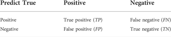
TABLE 1. Classification determination.

3 An improved biGRU based on LATC and Borderline-SMOTE algorithms

The experiments are organized into four parts. To evaluate the performance of the LATC algorithm in the incomplete dataset, the first experiment uses the MAPE and RMSE. The second part adopts the precision, recall rate, and f1-score indexes in order to evaluate the performance of the Borderline-SMOTE algorithm dealing with the class imbalance issue. The third part utilizes the accuracy and the same indexes used in the second part to evaluate the classification performance of the biGRU algorithm based on the attention mechanism in the Iris dataset and Wine dataset. Finally, the electric dataset of the UCI database is utilized to evaluate the classification performance of the proposed improved deep learning method. The details of the experimental environment are listed in Table 2.

TABLE 2

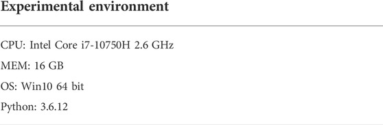
TABLE 2. Details of the experimental environment.

3.1 Study of the LATC algorithm

In this part, the subset of the electric dataset (Dua and Graff, 2019) of the UCI database is utilized to study the accuracy and efficiency of the LATC algorithm in completing the missing data. The details of the dataset are shown in Table 3. The subset of 321 users in 5 weeks is adopted from the original dataset in experiments. The cubic spline interpolation and quadratic interpolation algorithms are also implemented to compare with the LATC algorithm. MAPE and RMSE are applied to evaluate the classification result.

TABLE 3

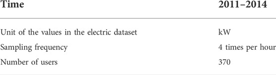
TABLE 3. Details of the subset of the electric dataset of the UCI database.

Figure 5 shows the MAPE and RMSE of classification results, which are obtained by different data completion methods with the rising loss rate. It can be seen that the performances of different completion methods with the low loss rate are quite close. However, as the loss rate rises, the LATC algorithm outperforms the other two methods. Especially, the RMSE of the cubic spline interpolation algorithm shows an exponential growth trend. It is worth noting that the large error can reduce the quality of the dataset, which will further lead to the failure of the classification to some extent. However, even when the loss rate reaches 90%, the MAPE of the LATC algorithm is still lower than 0.2, which can help the dataset classify successfully as soon as possible. In addition, the efficiency of completion results is shown in Table 4. It can be seen that the efficiency of LATC is lower than that of others. However, due to the outstanding completion ability, LATC can find a compromise between the accuracy and efficiency.

FIGURE 5

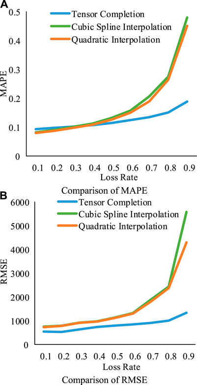
FIGURE 5. The (A) MARE and (B) RMSE of data completion methods with the rising loss rate.

TABLE 4

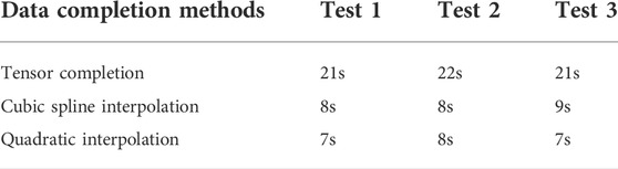
TABLE 4. Comparison of data completion methods in the efficiency.

3.2 Study of the Borderline-SMOTE algorithm

This section first uses the Iris dataset (Fisher, 2019a), which has the low-dimensional feature to evaluate the Borderline-SMOTE algorithm. SMOTE and ADASYN (adaptive synthetic sampling approach for imbalanced learning) algorithms are also implemented for comparison. However, the number of classes in the original Iris dataset is quite average, which is unable to evaluate the class balance methods directly. Therefore, the original Iris dataset needs to be processed to obtain the class-imbalanced Iris dataset. The details of the class-imbalanced Iris dataset and the dataset after the class balance methods processing are shown in Table 5. Subsequently, the GRU algorithm is applied to directly judge which category the new instances belong to. Eventually, the precision, recall rate, and f1-score are used to evaluate the performance of different class-balanced methods.

TABLE 5

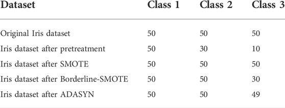
TABLE 5. Details of the class imbalanced Iris dataset and the dataset after the class balance methods processing.

From Table 6, it can be emphasized that all three algorithms perform stably. Although the recall rate of SMOTE/ADASYN in class 2 is 0.88/0.93, its evaluation result in other classes can reach a high level. In addition, it can be seen that in dealing with the low-dimensional dataset, the performances of all three methods are quite close. Especially, the class imbalance process result of the Borderline-SMOTE algorithm has the highest precision/recall rate/f1-score, the average of which is 1.

TABLE 6

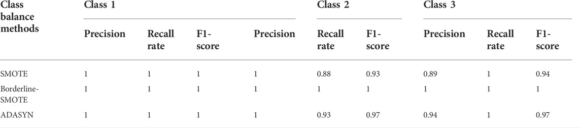
TABLE 6. Comparison of class balance methods with different classes using the Iris dataset.

In order to further evaluate the performance of the Borderline-SMOTE algorithm in terms of dealing with the high-dimensional class imbalanced dataset, the Wine dataset (Chen et al., 2021) is utilized. Different from the Iris dataset, the class imbalance issue already exists in the original Wine dataset. Therefore, the Wine dataset can be processed directly by class balance methods. The details of the Wine dataset and the dataset after the class balance method processing are shown in Table 7.

TABLE 7

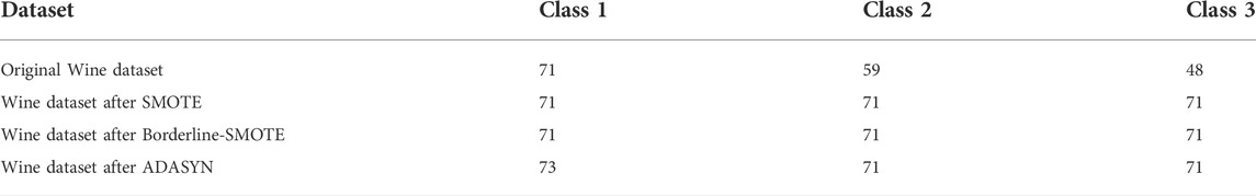
TABLE 7. Details of the Wine dataset and the dataset after the class balance methods processing.

The precision, recall rate, and f1-score of class balance methods using the Wine dataset are shown in Table 8. From Table 8, it can be seen that although the average recall rate of the SMOTE/ADASYN algorithm is 0.85/0.92, its minimal recall rate is only 0.64/0.83 in the experiment. In addition, the minimal precision and f1-score of the SMOTE/ADASYN algorithm are, respectively, 0.73/0.83 and 0.74/0.83, though its average precision and f1-score are more than 0.85. Therefore, compared with the low-dimensional Iris dataset, SMOTE and ADASYN algorithms lack the ability to deal with the higher-dimensional dataset stably. Moreover, the average precision/recall rate/f1-score of the Borderline-SMOTE algorithm can reach 0.97. Therefore, in terms of weakening the high-dimensional class imbalance, the performance of the Borderline-SMOTE algorithm is remarkably better than that of the ADASYN algorithm and subsequently better than the SMOTE algorithm.

TABLE 8

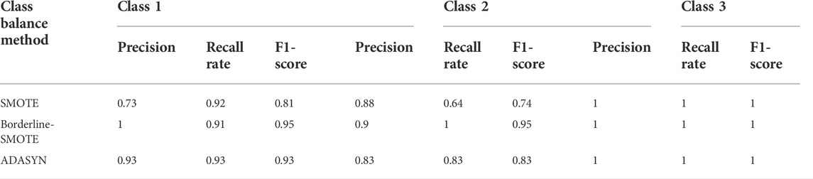
TABLE 8. Comparison of class balance methods with different classes using the Wine dataset.

3.3 Study of the attention mechanism–integrated biGRU algorithm

The Iris dataset (Fisher, 2019a) is used to study the performance of the biGRU with the attention mechanism algorithm. The training and the testing instances are randomly generated. The numbers of training and the testing instances of the Iris dataset are shown in Table 9. In order to compare with the attention mechanism–integrated biGRU algorithm, the attention mechanism–integrated RNN, LSTM, GRU, and biLSTM algorithms are also implemented.

TABLE 9

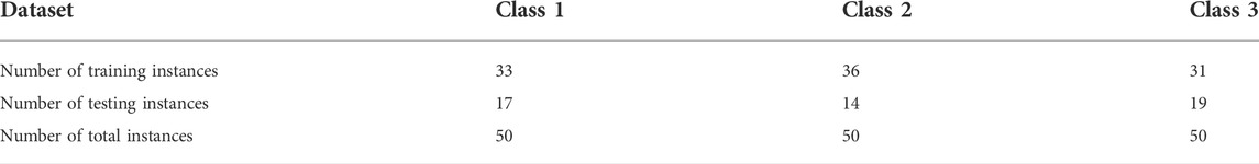
TABLE 9. Numbers of training and the testing instances of the Iris dataset.

Figure 6 shows the loss and accuracy of RNN, LSTM, GRU, and biLSTM with the attention mechanism algorithms and the proposed algorithm. It can be seen that the aforementioned five methods can classify the Iris dataset effectively. Especially, the loss of the RNN algorithm has an obvious downward trend. In addition, benefiting from the simple features in the Iris dataset, the accuracy of the RNN algorithm is 0.93 in the 10th epoch. Table 10 shows the precision, recall rate, and f1-score of load classification methods in different classes. It can be seen that the LSTM algorithm performs the most unstably for Iris. Although the LSTM algorithm precision of classes 1 and 2 are both 1, the precision of class 3 only has 0.70. Also, the LSTM algorithm recall rate/f1-score of class 2 is only 0.43/0.6, which is the least desirable result in the whole comparison. Compared with the LSTM algorithm, the average precision/recall rate/f1-score of other load classification is more than 0.9. Especially, it should be noted that the biGRU with the attention mechanism algorithm obviously outperforms the other classification methods, the average precision of which reaches 0.983.

FIGURE 6

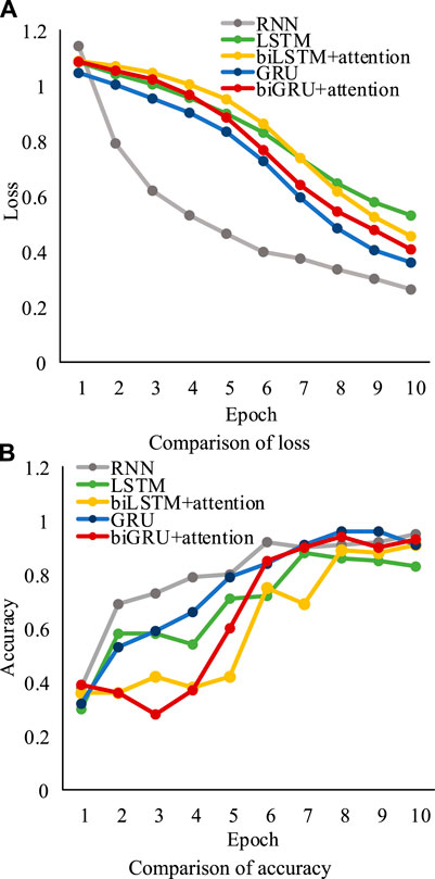
FIGURE 6. The (A) Loss and (B) Accuracy of load classification methods using the Iris dataset.

TABLE 10

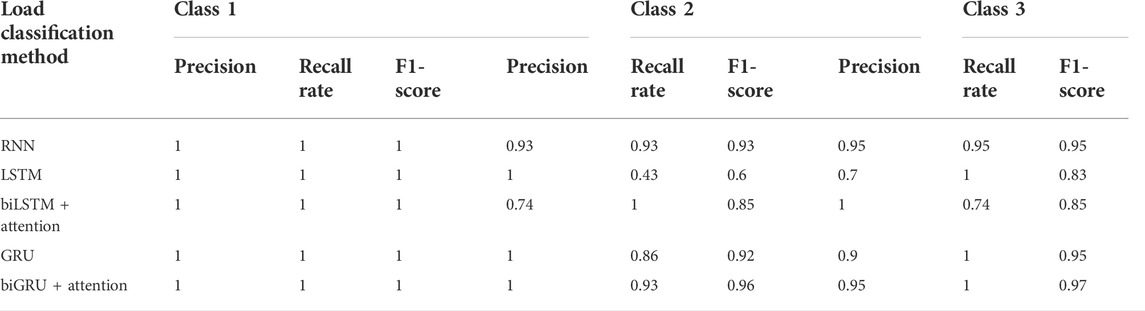
TABLE 10. Comparison of precision of load classification methods in different classes using the Iris dataset.

In addition, the Wine dataset (Aeberhard, 2019b) with higher-dimensional samples is further applied to evaluate the performance of the biGRU algorithm based on the attention mechanism. The details of the training and testing datasets are shown in Table 11.

TABLE 11

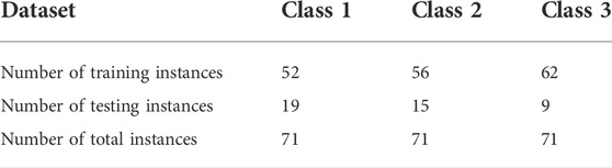
TABLE 11. Numbers of training and testing instances of the Wine dataset.

Figure 7 shows that high dimension severely influences the performance of the classification methods. Although the RNN algorithm performs well in the Iris experiment, its accuracy in the Wine dataset classification task is less than 0.70, which strongly suggests that the RNN algorithm lacks the ability of dealing with the high-dimensional dataset. However, compared with the RNN algorithm, the LSTM/GRU algorithm shows a better performance in preprocessing the Wine dataset. Table 12 further shows that the the RNN algorithm classifies the high-dimensional dataset unstably, especially in class 2. It is emphasized that biGRU with the attention mechanism algorithm shows excellent and stable classification ability. In terms of classification precision, recall rate, and f1-score, the GRU algorithm–based models outperform the other models. Especially, the biGRU algorithm based on the attention mechanism shows the greatest classification ability. The average of its precision/recall rate/f1-score reaches 0.98, while others are less than 0.95.

FIGURE 7

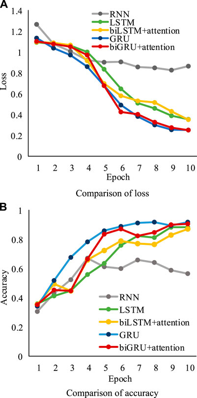
FIGURE 7. The (A) Loss and (B) Accuracy of load classification methods using the Wine dataset.

TABLE 12

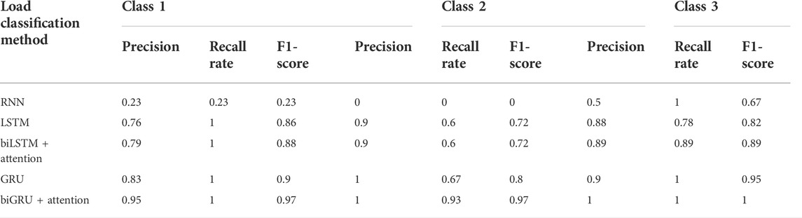
TABLE 12. Comparison of precision of load classification methods with different classes using the Wine dataset.

3.4 Study of the improved deep learning algorithm

To entirely evaluate the proposed improved deep learning algorithm, this part uses the complicated electric dataset (Dua and Graff, 2019) of the UCI database. This section randomly selects a part of the dataset, which includes the load data in 2 weeks of 196 users. However, the selected dataset only contains the real user load data without its corresponding label. Therefore, the unsupervised learning is adopted to obtain the labels (Gu and Iyer, 2017; Hussein et al., 2019). Finally, four experiments are designed to study the availability of the improved deep learning algorithm:

1) The biGRU algorithm with the attention mechanism.

2) The biGRU algorithm with the attention mechanism and LATC algorithm.

3) The biGRU algorithm with the attention mechanism and Borderline-SMOTE algorithm.

4) The proposed improved deep learning algorithm.

The precision, the recall rate, and the f1-score of different experiments are shown in Figure 8. From Figure 8, it can be seen that although all methods have the ability to accurately classify the dataset, the improved deep learning algorithm outperforms the others. It is worth noting that the methods without the class imbalance processing (experiments 1 and 2) have a weaker classification ability than the methods with the Borderline-SMOTE algorithm (experiments 3 and 4). Especially in experiment 2, the precision of the fourth class is only 0.63. The reason is that the class balancing processing highlights the feature of the minority data, which is quite helpful to distinguish the minority and majority. Consequently, the classification precision is dramatically improved. Meanwhile, the methods with the LATC algorithm (experiments 2 and 4) have weaker classification abilities than the methods without it (experiments 1 and 3). The reason is that missing data cause a decrease of the characteristics in the dataset, which leads to a low precision in the classification. The comparison of training and testing time of different methods are shown in Figure 9. It can be seen that although the class-balanced methods can effectively improve the precision, the run-time of classification algorithms based on class-balanced methods will rise sharply. The run-time of experiments 3 and 4 is more than 200s, while the run-time of experiments 1 and 2 is 70s. Therefore, it can be interpreted that the Borderline-SMOTE algorithm improves the classification precision; however, it generates more overheads.

FIGURE 8

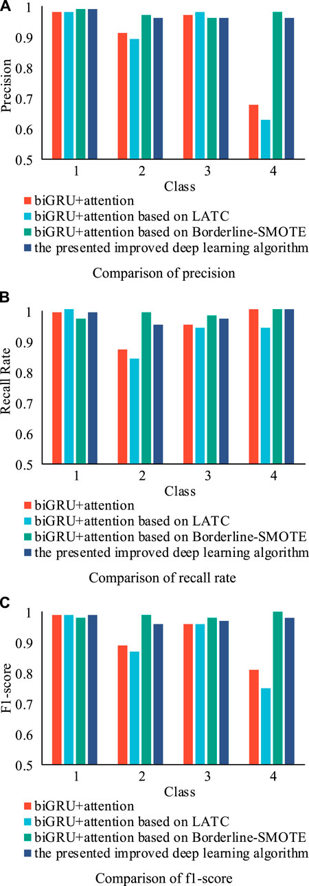
FIGURE 8. The (A) Precision a, (B) Recall Rate and (C) F1-score of different experiments with different classes.

FIGURE 9

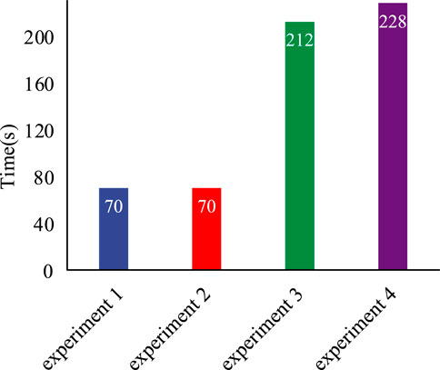
FIGURE 9. Comparison of time of different experiments.

The average precisions, the recall rates, and the f1-scores of different experiments are shown in Table 13. The average precision in experiment 3 reaches 0.99 while it is 0.98 in experiment 4. This is because the data completion algorithm will enrich the complexity and characteristics of the dataset. Therefore, the dataset after the completion may spend more training and testing time. Although the performance of the improved deep learning algorithm is worse than experiment 3 in terms of the precision, recall rate, and f1-score, its classification result is closer to reality with the balancing processing.

TABLE 13

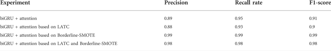
TABLE 13. Average of evaluation indexes of different experiments.

As a result, the test dataset is classified into four categories. The category mean center model (Gu and Iyer, 2017) is further used to analyze the load micro fluctuation at each moment. The comparison of category centers in different experiments is shown in Figure 9.

Figure 10A indicates that the load curve of category 1 shows a weak fluctuation. In addition, most load data belonging to category 1 are at a low level.

FIGURE 10

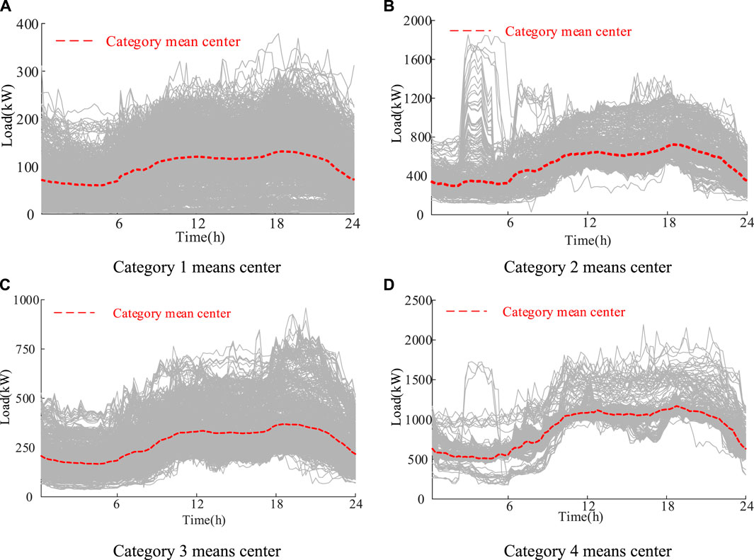
FIGURE 10. The load mean centers of (A) category 1, (B) category 2, (C) category 3 and (D) category 4.

Figure 10B indicates that the load curve of category 2 shows a strong fluctuation. Especially, some users in the 3 h or 4 h have a sudden increase in load. The highest load can reach 1800 kW.

Figure 10C indicates that the load curve of category 3 shows the same fluctuation as that of category 1. However, different from category 1, the average load of category 3 is about 250 kW.

Figure 10D indicates that the load curve of category 4 shows the strongest fluctuation in the whole category. It can be seen that some load curves in 3 h–6 h and 12 h–20 h in category 4 have an intense fluctuation. Especially, the highest load of the category 4 is more than 2000 kW.

Above all, the proposed deep learning algorithm can achieve a high precision, recall rate, and f1-score classification. In addition, the classification result shows the different features of each category.

4 Conclusion

This study proposed an improved deep learning algorithm in enabling load data classification for the power system. The algorithm first completes the missing dataset using the LATC algorithm, which not only improves the quality of the training dataset but also enriches the characteristics of the training dataset. Afterward, the Borderline-SMOTE algorithm is used to handle the class imbalance issue. The algorithm only generates the new samples for the borderline samples of the minority class to improve the class distribution. Also then, the attention mechanism is an integrated biGRU algorithm to further improve the accuracy and the recall rate. At last, this study designed four experiments to verify the effectiveness of the presented algorithm. The first experiment is designed to verify the great accuracy of LATC in data completion field. The second experiment uses the recall rate to prove the ability of tackling the imbalanced issue of Borderline-SMOTE. The third experiment adopts the Iris and Wine datasets to evaluate the classification performance of the biGRU based on the attention mechanism. The UCI dataset is used to verify the effectiveness of the presented algorithm in the last experiment. Based on the experimental results, the presented method outperforms most of the deep learning methods. Although this study proves that the presented algorithm shows a remarkable advantage in processing the load data, we need to point out that the disadvantage of the presented algorithm is the time cost in the training phase, which can be focused on in future research. Therefore, we consider to integrating ensemble learning with the presented algorithm in distributed computing, which will help the presented algorithm deal with the load data efficiently and accurately.

Data availability statement

Publicly available datasets were analyzed in this study. These data can be found here: http://archive.ics.uci.edu/ml/datasets/ElectricityLoadDiagrams20112014.

Author contributions

ZW and HL conceived the idea of the study; YL analyzed the data; SW interpreted the results. All authors were involved in writing the manuscript.

Conflict of interest

The authors declare that the research was conducted in the absence of any commercial or financial relationships that could be construed as a potential conflict of interest.

Publisher’s note

All claims expressed in this article are solely those of the authors and do not necessarily represent those of their affiliated organizations, or those of the publisher, the editors, and the reviewers. Any product that may be evaluated in this article, or claim that may be made by its manufacturer, is not guaranteed or endorsed by the publisher.

References

Aeberhard, S. (2019b). Wine Dataset. Available at http://archive.ics.uci.edu/ml/datasets/Wine.

Google Scholar

Alam, M. M., Shahjalal, M., Islam, M. M., Hasan, M. K., Ahmed, M. F., and Jang, Y. M. (2020). Power Flow Management with Demand Response Profiles Based on User-Defined Area, Load, and Phase Classification. IEEE Access 8, 218813–218827. doi:10.1109/ACCESS.2020.3041841

CrossRef Full Text | Google Scholar

Almuzaini, H. A., and Azmi, A. M. (2020). Impact of Stemming and Word Embedding on Deep Learning-Based Arabic Text Categorization. IEEE Access 8, 127913–127928. doi:10.1109/access.2020.3009217

CrossRef Full Text | Google Scholar

Aref, Y., Cemal, K., Asef, Y., and Amir, S. (2020). Automatic Fuzzy-DBSCAN Algorithm for Morphological and Overlapping Datasets. J. Syst. Eng. Electron. 31 (6), 1245–1253. doi:10.23919/JSEE.2020.000095

CrossRef Full Text | Google Scholar

Azarkhail, M., and Woytowitz, P. (2013). “Uncertainty Management in Model-Based Imputation for Missing Data,” in Proceedings Annual Reliability and Maintainability Symposium (RAMS), 1–7.

CrossRef Full Text | Google Scholar

Cai, Q., Liu, S., and Lu, Q. (2017). Identification Method for User Industry Classification Based on GMM Clustering and SVM. Guangdong Electr. Power, 91–96.

Google Scholar

Chen, X., and Sun, L. (2020). Low-Rank Autoregressive Tensor Completion for Multivariate Time Series Forecasting.

Google Scholar

Chen, Y., Chang, R., and Guo, J. (2021). Effects of Data Augmentation Method Borderline-SMOTE on Emotion Recognition of EEG Signals Based on Convolutional Neural Network. IEEE Access 9, 47491–47502. doi:10.1109/access.2021.3068316

CrossRef Full Text | Google Scholar

Chu, H. (2011). Applied Missing Data Analysis. The American statistician, 201.

Google Scholar

Deng, W., Guo, Y., Liu, J., Li, Y., Liu, D., and Zhu, L. (2019). A Missing Power Data Filling Method Based on Improved Random Forest Algorithm. Chin. J. Electr. Eng. 5 (4), 33–39. doi:10.23919/cjee.2019.000025

CrossRef Full Text | Google Scholar

Dharmasaputro, A. A., Fauzan, N. M., Kallista, M., Wibawa, I. P. D., and Kusuma, P. D. (2022). “Handling Missing and Imbalanced Data to Improve Generalization Performance of Machine Learning Classifier,” in 2021 International Seminar on Machine Learning, Optimization, and Data Science (ISMODE), 140–145. doi:10.1109/ISMODE53584.2022.9743022

CrossRef Full Text | Google Scholar

Dogo, E. M., Nwulu, N. I., Twala, B., and Aigbavboa, C. O. (2020). Empirical Comparison of Approaches for Mitigating Effects of Class Imbalances in Water Quality Anomaly Detection. IEEE Access 8, 218015–218036. doi:10.1109/ACCESS.2020.3038658

CrossRef Full Text | Google Scholar

Dongsong, Z., and Qi, M. (2017). “A Load Identification Algorithm Based on SVM,” in 2017 First International Conference on Electronics Instrumentation & Information Systems (EIIS), 1–5.

CrossRef Full Text | Google Scholar

Du, M., Gao, J., Zhang, L., Luo, M., Chen, Y., Hu, W., et al. (2020). Time Series Forecasting and Imputation of Dam Physical Quantities. Water Power, 111–115.

Google Scholar

Dua, D., and Graff, C. (2019). UCI Machine Learning Repository. Available at http://archive.ics.uci.edu/ml/datasets/ElectricityLoadDiagrams20112014.

Google Scholar

Ebenuwa, S. H., Sharif, M. S., Alazab, M., and Al-Nemrat, A. (2019). Variance Ranking Attributes Selection Techniques for Binary Classification Problem in Imbalance Data. IEEE Access 7, 24649–24666. doi:10.1109/access.2019.2899578

CrossRef Full Text | Google Scholar

Fisher, R. A. (2019a). Iris Dataset. Available at https://archive.ics.uci.edu/ml/datasets/Iris.

Google Scholar

Ghorbani, R., and Ghousi, R. (2020). Comparing Different Resampling Methods in Predicting Students’ Performance Using Machine Learning Techniques. IEEE Access 8, 67899–67911. doi:10.1109/ACCESS.2020.2986809

CrossRef Full Text | Google Scholar

Gramajo, M., Ballejos, L., and Ale, M. (2020). Seizing Requirements Engineering Issues through Supervised Learning Techniques. IEEE Lat. Am. Trans. 18 (07), 1164–1184. doi:10.1109/TLA.2020.9099757

CrossRef Full Text | Google Scholar

Greff, K., Srivastava, R. K., Koutník, J., Steunebrink, B. R., and Schmidhuber, J. (2017). LSTM: A Search Space Odyssey. IEEE Trans. Neural Netw. Learn. Syst. 28 (10), 2222–2232. doi:10.1109/tnnls.2016.2582924

PubMed Abstract | CrossRef Full Text | Google Scholar

Gu, X., and Iyer, S. S. (2017). Unsupervised Learning Using Charge-Trap Transistors. IEEE Electron Device Lett. 38 (9), 1204–1207. doi:10.1109/led.2017.2723319

CrossRef Full Text | Google Scholar

Guo, A. J. X., and Zhu, F. (2019). Spectral-Spatial Feature Extraction and Classification by ANN Supervised with Center Loss in Hyperspectral Imagery. IEEE Trans. Geosci. Remote Sens. 57 (3), 1755–1767. doi:10.1109/tgrs.2018.2869004

CrossRef Full Text | Google Scholar

Harishma, B., Mathew, P., Patranabis, S., Chatterjee, U., Agarwal, U., Maheshwari, M., et al. (2022). Safe Is the New Smart: PUF-Based Authentication for Load Modification-Resistant Smart Meters. IEEE Trans. Dependable Secure Comput. 19 (1), 663–680. doi:10.1109/TDSC.2020.2992801

CrossRef Full Text | Google Scholar

Hong, Y. -Y., and Hsiao, C. -Y. (2022). Under-Frequency Load Shedding in a Standalone Power System with Wind-Turbine Generators Using Fuzzy PSO. IEEE Trans. Power Deliv. 37 (2), 1140–1150. doi:10.1109/TPWRD.2021.3077668

CrossRef Full Text | Google Scholar

Hongbo, Q., Yanqi, W., and Ran, Y. (2019). The Influence of Unbalance Load on the Electromagnetic and Temperature Field of High-Speed Permanent Magnet Generator. IEEE Trans. Magn. 55 (6), 1–4. doi:10.1109/TMAG.2018.2886434

CrossRef Full Text | Google Scholar

Hosseini, S. M., and Sebt, M. A. (2017). Array Interpolation Using Covariance Matrix Completion of Minimum-Size Virtual Array. IEEE Signal Process. Lett. 24 (7), 1063–1067. doi:10.1109/LSP.2017.2708750

CrossRef Full Text | Google Scholar

Hu, F., Zhu, C., and Wang, Z. (2018). Research on the Power Load Classification Based on Improved K-Means Algorithm. Electron. Meas. Technol., 44–48.

Google Scholar

Hussein, S., Kandel, P., Bolan, C. W., Wallace, M. B., and Bagci, U. (2019). Lung and Pancreatic Tumor Characterization in the Deep Learning Era: Novel Supervised and Unsupervised Learning Approaches. IEEE Trans. Med. Imaging 38 (8), 1777–1787. doi:10.1109/tmi.2019.2894349

PubMed Abstract | CrossRef Full Text | Google Scholar

Jeon, Y., and Lim, D. (2020). PSU: Particle Stacking Undersampling Method for Highly Imbalanced Big Data. IEEE Access 8, 131920–131927. doi:10.1109/ACCESS.2020.3009753

CrossRef Full Text | Google Scholar

Jia, Y., Dong, Z. Y., Sun, C., and Meng, K. (2019). Cooperation-Based Distributed Economic MPC for Economic Load Dispatch and Load Frequency Control of Interconnected Power Systems. IEEE Trans. Power Syst. 34 (5), 3964–3966. doi:10.1109/TPWRS.2019.2917632

CrossRef Full Text | Google Scholar

Jing, X., Wu, F., Dong, X., and Xu, B. (2017). An Improved SDA Based Defect Prediction Framework for Both Within-Project and Cross-Project Class-Imbalance Problems. IIEEE. Trans. Softw. Eng. 43 (4), 321–339. doi:10.1109/tse.2016.2597849

CrossRef Full Text | Google Scholar

Le, T., Kim, J., and Kim, H. (2016). “Classification Performance Using Gated Recurrent Unit Recurrent Neural Network on Energy Disaggregation,” in International Conference on Machine Learning and Cybernetics (ICMLC), 105–110.

CrossRef Full Text | Google Scholar

Lee, G. S., Bang, S. S., Mantooth, H. A., and Shin, Y. -J. (2020). Condition Monitoring of 154 kV HTS Cable Systems via Temporal Sliding LSTM Networks. IEEE Access 8, 144352–144361. doi:10.1109/access.2020.3014227

CrossRef Full Text | Google Scholar

Lepolesa, L. J., Achari, S., and Cheng, L. (2022). Electricity Theft Detection in Smart Grids Based on Deep Neural Network. IEEE Access 10, 39638–39655. doi:10.1109/ACCESS.2022.3166146

CrossRef Full Text | Google Scholar

Li, Q., Tan, H., Wu, Y., Ye, L., and Ding, F. (2020). Traffic Flow Prediction with Missing Data Imputed by Tensor Completion Methods. IEEE Access 8, 63188–63201. doi:10.1109/access.2020.2984588

CrossRef Full Text | Google Scholar

Lin, S., Li, F., Tian, E., Fu, Y., and Li, D. (2019). Clustering Load Profiles for Demand Response Applications. IEEE Trans. Smart Grid 10 (2), 1599–1607. doi:10.1109/tsg.2017.2773573

CrossRef Full Text | Google Scholar

Liu, W., Liu, H., Wang, F., Wang, C., Zhao, L., and Wang, H. (2020). Practical Automatic Planning for MV Distribution Network Considering Complementation of Load Characteristic and Power Supply Unit Partitioning. IEEE Access 8, 91807–91817. doi:10.1109/ACCESS.2020.2966010

CrossRef Full Text | Google Scholar

Liu, Z., Xiao, Z., Wu, Y., Hou, H., Xu, T., Zhang, Q., et al. (2021). Integrated Optimal Dispatching Strategy Considering Power Generation and Consumption Interaction. IEEE Access 9, 1338–1349. doi:10.1109/access.2020.3045151

CrossRef Full Text | Google Scholar

Marchang, N., and Tripathi, R. (2021). KNN-ST: Exploiting Spatio-Temporal Correlation for Missing Data Inference in Environmental Crowd Sensing. IEEE Sens. J. 21 (3), 3429–3436. doi:10.1109/jsen.2020.3024976

CrossRef Full Text | Google Scholar

Niu, D., Wanq, Q., and Li, J. (2005). “Short Term Load Forecasting Model Using Support Vector Machine Based on Artificial Neural Network,” in International Conference on Machine Learning and Cybernetics, 4260–4265.

Google Scholar

Oslebo, D., Corzine, K., Weatherford, T., Maqsood, A., and Norton, M. (2019). “DC Pulsed Load Transient Classification Using Long Short-Term Memory Recurrent Neural Networks,” in 2019 13th International Conference on Signal Processing and Communication Systems (ICSPCS), 1–6.

CrossRef Full Text | Google Scholar

Pan, M., Zhou, H., Cao, J., Liu, Y., Hao, J., Li, S., et al. (2020). Water Level Prediction Model Based on GRU and CNN. IEEE Access 8, 60090–60100. doi:10.1109/access.2020.2982433

CrossRef Full Text | Google Scholar

Park, K., Jeong, J., Kim, D., and Kim, H. (2020). Missing-Insensitive Short-Term Load Forecasting Leveraging Autoencoder and LSTM. IEEE Access 8, 206039–206048. doi:10.1109/access.2020.3036885

CrossRef Full Text | Google Scholar

Peng, X., Lai, J., and Chen, Y. (2014). Application of Clustering Analysis in Typical Power Consumption Profile Analysis. Power Syst. Prot. Control, 68–73.

Google Scholar

Phyo, P. P., and Jeenanunta, C. (2021). Daily Load Forecasting Based on a Combination of Classification and Regression Tree and Deep Belief Network. IEEE Access 9, 152226–152242. doi:10.1109/ACCESS.2021.3127211

CrossRef Full Text | Google Scholar

Polat, K. (2019). A Hybrid Approach to Parkinson Disease Classification Using Speech Signal: The Combination of SMOTE and Random Forests. Sci. Meet. Electrical-Electronics Biomed. Eng. Comput. Sci. (EBBT), 1–3.

CrossRef Full Text | Google Scholar

Ross, S., and Mathieu, J. (2021). Strategies for Network-Safe Load Control with a Third-Party Aggregator and a Distribution Operator. IEEE Trans. Power Syst. 36 (4), 3329–3339. doi:10.1109/TPWRS.2021.3052958

CrossRef Full Text | Google Scholar

Sajjad, M., Khan, Z. A., Ullah, A., Hussain, T., Ullah, W., Lee, M. Y., et al. (2020). A Novel CNN-GRU-Based Hybrid Approach for Short-Term Residential Load Forecasting. IEEE Access 8, 143759–143768. doi:10.1109/access.2020.3009537

CrossRef Full Text | Google Scholar

Saravanan, R., and Sujatha, P. (2018). “A State of Art Techniques on Machine Learning Algorithms: A Perspective of Supervised Learning Approaches in Data Classification,” in 2018 Second International Conference on Intelligent Computing and Control Systems (ICICCS), 945–949.

CrossRef Full Text | Google Scholar

Sinaga, K. P., and Yang, M. (2020). Unsupervised K-Means Clustering Algorithm. IEEE Access 8, 80716–80727. doi:10.1109/ACCESS.2020.2988796

CrossRef Full Text | Google Scholar

Su, Y., Wu, X., and Liu, W. (2019). Low-Rank Tensor Completion by Sum of Tensor Nuclear Norm Minimization. IEEE Access 7, 134943–134953. doi:10.1109/ACCESS.2019.2940664

CrossRef Full Text | Google Scholar

Sun, H., Yi, J., Xu, Y., Wang, Y., and Qing, X. (2019). Crack Monitoring for Hot-Spot Areas under Time-Varying Load Condition Based on FCM Clustering Algorithm. IEEE Access 7, 118850–118856. doi:10.1109/ACCESS.2019.2936554

CrossRef Full Text | Google Scholar

Sun, R., Xiao, X., Zhou, F., and Zhou, Y. (2019). “Research of Power User Load Classification Method Based on K-Means and FSVM,” in 2019 IEEE 3rd Information Technology, Networking, Electronic and Automation Control Conference (ITNEC), 2138–2142.

Google Scholar

Tian, Y., and Compere, M. (2019). “A Case Study on Visual-Inertial Odometry Using Supervised, Semi-supervised and Unsupervised Learning Methods,” in 2019 IEEE International Conference on Artificial Intelligence and Virtual Reality (AIVR), 203–2034.

CrossRef Full Text | Google Scholar

Ullah, S., Khan, L., Sami, I., and Ro, J. -S. (2022). Voltage/Frequency Regulation with Optimal Load Dispatch in Microgrids Using SMC Based Distributed Cooperative Control. IEEE Access 10, 64873–64889. doi:10.1109/ACCESS.2022.3183635

CrossRef Full Text | Google Scholar

Wang, J., and Wang, C. (2005). “Bayes Method of Power Quality Disturbance Classification,” in TENCON 2005 - 2005 IEEE Region 10 Conference, 1–4.

CrossRef Full Text | Google Scholar

Wang, Q., Cao, W., Guo, J., Ren, J., Cheng, Y., and Davis, D. N. (2019). DMP_MI: An Effective Diabetes Mellitus Classification Algorithm on Imbalanced Data with Missing Values. IEEE Access 7, 102232–102238. doi:10.1109/ACCESS.2019.2929866

CrossRef Full Text | Google Scholar

Wang, X., Tang, Q., Wang, H., Ma, R., and Tang, Z. (2020). “High-performance Machine Learning in Enabling Large-Scale Load Analysis Considering Class Imbalance and Frequency Domain Characteristics,” in 2020 IEEE Sustainable Power and Energy Conference (iSPEC), 2411–2416.

CrossRef Full Text | Google Scholar

Xu, Q., Ding, Y., Yan, Q., Zheng, A., and Du, P. (2017). Day-Ahead Load Peak Shedding/Shifting Scheme Based on Potential Load Values Utilization: Theory and Practice of Policy-Driven Demand Response in China. IEEE Access 5, 22892–22901. doi:10.1109/access.2017.2763678

CrossRef Full Text | Google Scholar

Xu, Y., Zhang, L., and Song, G. (2015). Application of Clustering Hierarchy Algorithm Based on Kernel Fuzzy C-Means in Power Load Classification. Electr. Power Constr., 46–51.

Google Scholar

Yang, H., Zhang, J., Qiu, J., Zhang, S., Lai, M., and Dong, Z. Y. (2018). A Practical Pricing Approach to Smart Grid Demand Response Based on Load Classification. IEEE Trans. Smart Grid 9 (1), 179–190. doi:10.1109/TSG.2016.2547883

CrossRef Full Text | Google Scholar

Yang, M., Lin, Y., and Han, X. (2016). Probabilistic Wind Generation Forecast Based on Sparse Bayesian Classification and Dempster–Shafer Theory. IEEE Trans. Ind. Appl. 52 (3), 1998. doi:10.1109/tia.2016.2518995

CrossRef Full Text | Google Scholar

Yao, Q., Liu, J., and Hu, Y. (2019). Optimized Active Power Dispatching Strategy Considering Fatigue Load of Wind Turbines during De-loading Operation. IEEE Access 7, 17439–17449. doi:10.1109/access.2019.2893957

CrossRef Full Text | Google Scholar

Yu, Y., Yu, J. J. Q., Li, V. O. K., and Lam, J. C. K. (2020). A Novel Interpolation-SVT Approach for Recovering Missing Low-Rank Air Quality Data. IEEE Access 8, 74291–74305. doi:10.1109/access.2020.2988684

CrossRef Full Text | Google Scholar

Yuan, L., Zhao, Q., and Cao, J. (2018). “High-Order Tensor Completion for Data Recovery via Sparse Tensor-Train Optimization,” in IEEE International Conference on Acoustics, Speech and Signal Processing (ICASSP), 1258–1262.

CrossRef Full Text | Google Scholar

Zhang, F., Liu, Q., Liu, Y., Tong, N., Chen, S., and Zhang, C. (2020). Novel Fault Location Method for Power Systems Based on Attention Mechanism and Double Structure GRU Neural Network. IEEE Access 8, 75237–75248. doi:10.1109/access.2020.2988909

CrossRef Full Text | Google Scholar

Zhang, L., Song, L., Du, B., and Zhang, Y. (2021). Nonlocal Low-Rank Tensor Completion for Visual Data. IEEE Trans. Cybern. 51 (2), 673–685. doi:10.1109/TCYB.2019.2910151

PubMed Abstract | CrossRef Full Text | Google Scholar

Zhang, X., Xie, X., Wang, Y., Zhang, X., Jiang, D., Yu, C., et al. (2020). A Digital Signage Audience Classification Model Based on the Huff Model and Backpropagation Neural Network. IEEE Access 8, 71708–71720. doi:10.1109/access.2020.2987717

CrossRef Full Text | Google Scholar

Zhu, X., Zhang, S., Jin, Z., Zhang, Z., and Xu, Z. (2011). Missing Value Estimation for Mixed-Attribute Data Sets. IEEE Trans. Knowl. Data Eng. 23 (1), 110–121. doi:10.1109/tkde.2010.99

CrossRef Full Text | Google Scholar