 Laiq Zada1
 Nasir Ali1
 Rashid Nawaz1
 Wasim Jamshed2*
 Mohamed R. Eid3,4El Sayed M. Tag El Din5Hamiden Abd El- Wahed Khalifa6,7Fayza Abdel Aziz ElSeabee8,9
- 1Department of Mathematics, Abdul Wali Khan University Mardan, Mardan, Pakistan
- 2Department of Mathematics, Capital University of Science and Technology (CUST), Islamabad, Pakistan
- 3Department of Mathematics, Faculty of Science, New Valley University, Al-Kharga, Al-Wadi Al-Gadid, Egypt
- 4Department of Mathematics, Faculty of Science, Northern Border University, Arar, Saudi Arabia
- 5Electrical Engineering, Faculty of Engineering and Technology, Future University in Egypt, New Cairo, Egypt
- 6Department of Operations Research, Faculty of Graduate Studies for Statistical Research, Cairo University, Giza, Egypt
- 7Department of Mathematics, College of Science and Arts, Qassim University, Al-Badaya, Saudi Arabia
- 8Mathematics Department, Faculty of Science, Helwan University, Cairo, Egypt
- 9Department of Mathematics, College of Science and Arts, Qassim University, Alasyah, Saudi Arabia
In the present study, the natural transform iterative method (NTIM) has been implemented for the solution of a fractional Zakharavo–Kuznetsov (FZK) equation. NTIM is a relatively new technique for handling non-linear fractional differential equations. The method is tested upon the two non-linear FZK equalities. The solution of the proposed technique has been compared with the existing perturbation–iteration algorithm (PIA) method and residual power series method (RPSM). From the numerical results, it is clear that the method handles non-linear differential equations very suitably and provides the results in very closed accord with the accurate solution. As a result, the NTIM approach is regarded as one of the finest analytical techniques for solving fractional-order linear and non-linear problems.
1 Introduction
Entropy and fractional calculus are appealing concepts that are increasingly being used to investigate the dynamics of complicated systems. Fractional calculus (FC) has been increasingly used in numerous sectors of research in recent years. Fractional differential equalities (FDEs) efficiently depict the natural evolution associated with viscoelasticity, models of porous electrodes, thermal stresses, electromagnetism, energy transmission in viscous dissipation systems, relaxing oscillations, and thermoelasticity. Most of the mathematical models are obtained through real-world problems which can be modeled via differential equations of the integer order or of the fractional order. The differential equations may arise in diverse areas of technological sciences and biological sciences. In engineering sciences, they may be in the field of fluid dynamics, aerodynamics, the nuclear decay, climate changes, electronic circuits, etc. In biosciences, these models may be of the blood flow, population growth, and decay problems of some kind of species of organisms like bacteria or virus and may be the study of some rate of flow of some gas models or may be the concentration control of some liquids in some other liquids. Similarly, differential equations may also model some problems related to social sciences as in the fields of banking and finance. The customer may be satisfied by preparing a fractional model of interest or premium according to the required efforts of a person. Fractional calculus plays an essential role in these kinds of problems.
Fractional calculation is the generalization of the classical calculus which is an ancient branch of mathematics. The fractional calculus received much more attention of researchers during the last few decades. Fractional calculus has great achievements in the fields of physics, engineering, biology, medicine, hydrology, economics, and finance [1-5]. The models of differential equations may be linear or nonlinear; linear models can be solved easily by different methods and do not require too much difficulty for obtaining the exact solution. But most of the problems of the real world occur non-linearly and cannot be solved easily. They are very hard to solve by simple methods. Most of the non-linear problems do not have exact solutions. Therefore, researchers use different approaches to solve them.
Researchers use numerical methods to solve non-linear problems, but they have discretization issue, are costly, and time-consuming. The famous numerical methods are the following: the collocation method, finite difference technique, finite element procedure, and radial basis function technique [6-8]. Similarly, perturbation methods need small or large parameter assumptions which are very difficult [9, 10]. Non-perturbation methods are the Adomian decomposition methodology (ADM) and differential transformation methodolgy (DTM). These methods work on repetition and that is why these types of problems can be solved with the help of computer software easily. Some well-known iterative methods are the variational iterating methodology (VIM), new iterating methodology, modified variational iteration method (MVIM), etc. [11, 12]. The Zakharov–Kuznetsov (ZK) equation is an enticing modeling formula for studying vortices in geophysics flows. The ZK difficulties appear in many areas of material sciences, implemented arithmetic, and design. It occurs particularly in the realm of physical sciences. The ZK issues govern the behavior of weak non-linear particle acoustic plasma waves, such as cold nanoparticles and hot adiabatic electrons, in the presence of smooth magnetism. The non-direct higher order of the expanded KdV criteria for geometrical removal was used to generate solitary wave configurations. The accurate expository structures of various non-linear advancement equations in numerical materials engineering, namely, space time-fractional Zakharov–Kuznetsov and altered Zakharov–Kuznetsov formulas, were found using a fractional technique. Many approaches, including the new iterating Sumudu understanding of the complex, homotopy perturbation transform method, expanded direct algebra methodology, natural decomposition technique, and q-homotopy analysis transform methodology, have been used to examine it during the last few decades. In this research work, we will find the approximate solution to the fractional order of the Zakharova–Kuznetsova FZK equation (13). The general form of the FZK equation is
where
2 Basic definitions
Definition 2.1 [14]: The fractional integral operator
where
Definition 2.2 [14]: Riemann–Liouville fractional derivative can be defined if
Some properties of the fractional derivative and integral are given as
Definition 2.3: Natural transubstantiate is specified as [18]
Definition 2.4 [18]: The inverse of the natural transubstantiate
Definition 2.5 [18]: If
Theorem 2.6: If
where
2.1 Natural Transform Iterative Method (NTIM)
Consider the fractional order PDE in the manner
where
Taking the natural transform of (7), we have
By employing the differentiate characteristic of the natural conversion to Eq. (9), we have
Using the initial condition and rearranging Eq. (10), we obtain
As the linear term
and
Applying Eq. (13) in Eq. (11), we obtain
The recursive relation of Eq. (14) by the use of natural transform is
Utilizing the inverted natural transmute to Eq. (15), the solution component can be obtained as
The
2.2 Convergence of the NTIM
Theorem 2.7 [18]: If
for any
To appear in the boundaries of
Theorem 2.8: If
3 Implementation of the NTIM to the FZK equation
Example 3.1. Consider the FZK equation in the following form [13]:
Together, the initial condition is
Eq. (18) is written in the implicit form as
Using natural conversion to Eq. (20), we get
Utilize the differentiation characteristic of the natural convert as
Using the initial condition in Eq. (20) and rearranging, we have
As
applying natural transform to Eq. (25) and using the idea explained in the method
(25)Now, by taking the inverted natural transmute of Eq. 25, we obtain the solution elements as
(26)The
Example 3.2. Regarding the FZK (2, 2, 2) equality of the structure [13]
With preliminary conditions
Here,
Utilizing the procedure of NTIM, we obtain the solution components for Eq. (28) as
Adding the elements, the second-order approximated solution can be written as
Example 3.3. Consider the FZK (3, 3, 3) equation of the structure [13]
Together with initial conditions
Here,
Using the procedure of the NTIM, the solution elements can be acquired as
(39)Adding the components, the second-order series solution can be written as
4 Results and discussion
In this work, two problems of the FZK equation have been tested by the new developed methodology NTIM. The obtained results are assessed by diverse plots and tabulated data for testing the reliability of the proposed method. Figure 1 shows the 3D surfaces obtained by the NTIM and the accurate result correspondingly for Example 3.2 in the 3D graph by keeping the y parameter constant. By keeping the time parameter constant, the approximate and accurate results are shown in Figure 2 respectively, for problem 3.2. In Figure 3, the absolute error is shown by a 3D plot by the variation of
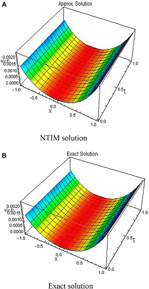
FIGURE 1. 3D plots obtained by the first order (A) NTIM and (B) exact solution for
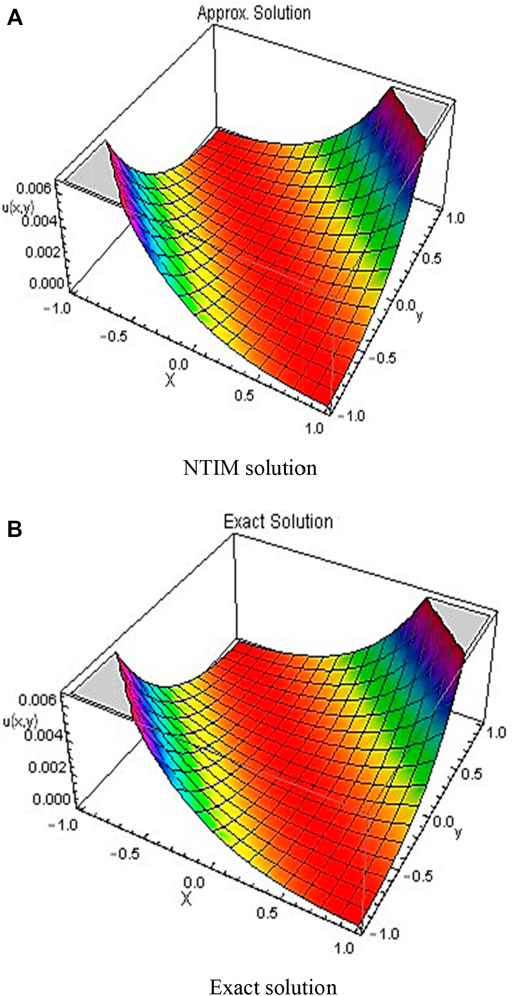
FIGURE 2. 3D plots obtained by the first order (A) NTIM and (B) exact solution for
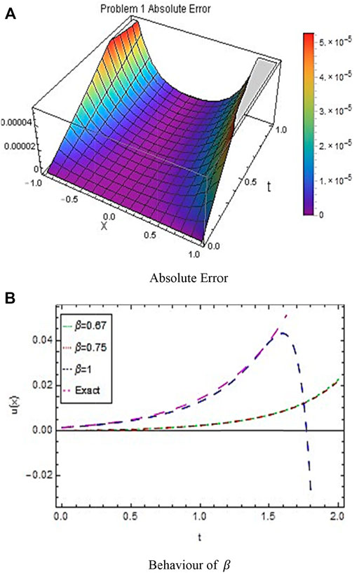
FIGURE 3. (A) shows the absolute error and (B) shows the behavior of
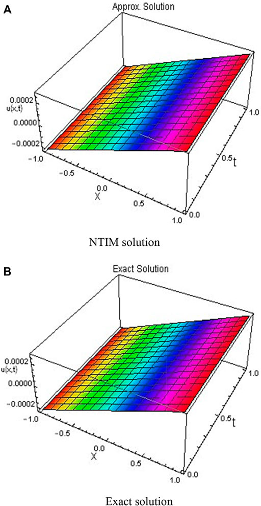
FIGURE 4. 3D plots obtained by the first order (A) NTIM and (B) exact solution for
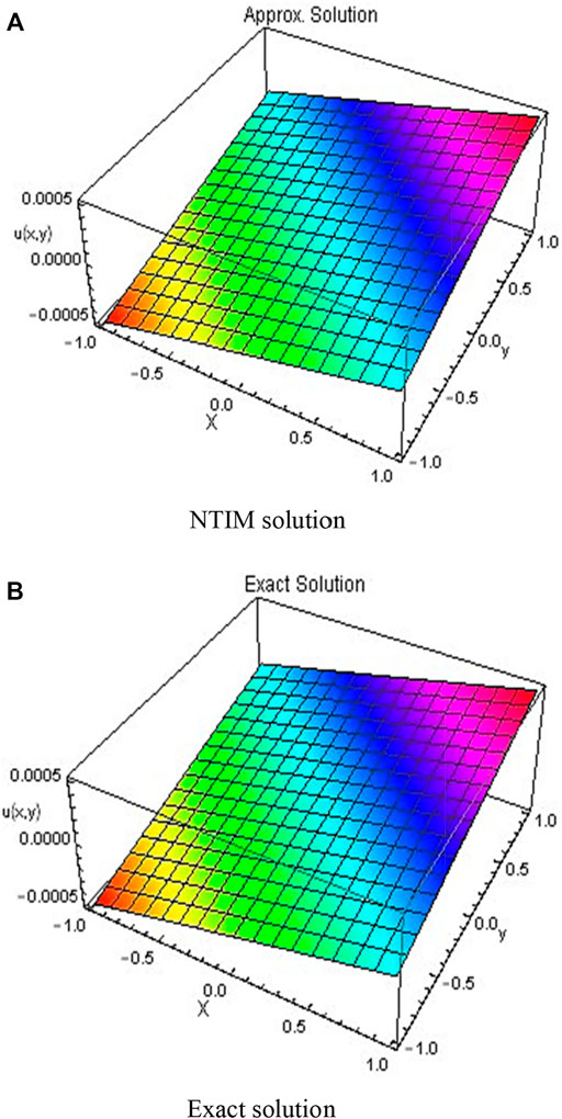
FIGURE 5. 3D plots obtained by the first order (A) NTIM and (B) exact solution for
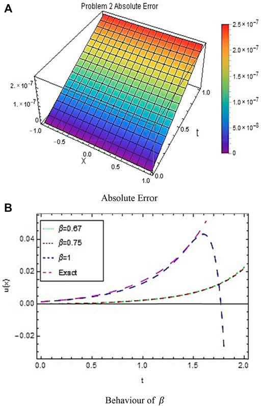
FIGURE 6. (A) shows the absolute error and (B) shows the behavior of

TABLE 1. Few important expressions and their natural transubstantiates.

TABLE 2. Comparison of the second-order NTIM with the third-order RPSM and PIA method for diverse amounts of
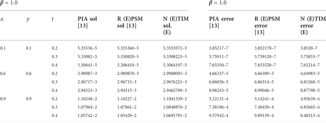
TABLE 3. Comparison of the second-order NTIM with the third-order RPSM and PIA method.
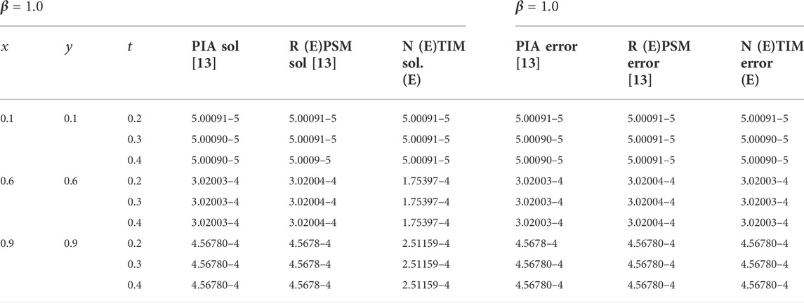
TABLE 4. Comparison of the second-order NTIM with the third-order RPSM and PIA method.
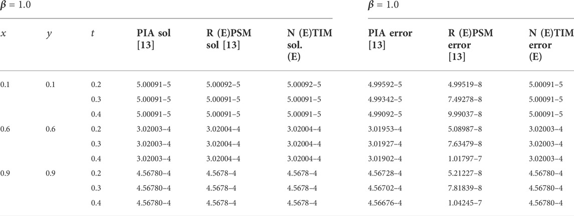
TABLE 5. Comparison of the second-order NTIM with the third-order RPSM and PIA method.
5. Conclusion
In the current investigation, the NTIM has been applied successfully to the FZK equations. Two problems have been tested. The proposed results reveal that the method handles the non-linear equations in a good way and provides an efficient approximate solution to non-linear PDEs. The numerical values of approximate and exact solutions through tables show the efficiency and reliability of the method. Also, the graphs verify the efficiency of the proposed method through 3D and 2D plots. The fractional approximation through 2D graphs also shows the consistency of the method by approaching the fractional value
Data availability statement
The original contributions presented in the study are included in the article/supplementary material; further inquiries can be directed to the corresponding author.
Author contributions
LZ and RN formulated the problem. NA and WJ solved the problem. LZ, NA, RN, WJ, MRE, ESMTED, HAEWK, and FAAE, computed and scrutinized the results. All the authors equally contributed in writing and proof reading of the paper. All authors reviewed the manuscript.
Acknowledgments
The researchers would like to thank the Deanship of Scientific Research, Qassim University for funding the publication of this project.
Conflict of interest
The authors declare that the research was conducted in the absence of any commercial or financial relationships that could be construed as a potential conflict of interest.
Publisher’s note
All claims expressed in this article are solely those of the authors and do not necessarily represent those of their affiliated organizations, or those of the publisher, the editors, and the reviewers. Any product that may be evaluated in this article, or claim that may be made by its manufacturer, is not guaranteed or endorsed by the publisher.
References
Gorenflo, R., and Mainardi, F. (2005). Simply and multiply scaled diffusion limits for continuous time random walks. J. Phys, Conf. Ser. 7, 1–16. doi:10.1088/1742-6596/7/1/001
Barkai, E., Metzler, R., and Klafter, J. (2000). From continuous time random walks to the fractional Fokker-Planck equation. Phys. Rev. E 61 (1), 132–138. doi:10.1103/physreve.61.132
Benson, D.A., Wheatcraft, S.W., and Meerschaert, M.M. (2000). Application of a fractional advection‐dispersion equation. Water Resour. Res. 36 (6), 1403–1412.
Almeida, R. (2017). A caputo fractional derivative of a function with respect to another function. Commun. Nonlinear Sci. Numer. Simul. 44, 460–481. doi:10.1016/j.cnsns.2016.09.006
Muslih, S., Baleanu, D., and Rabei, E. (2007). Gravitational potential in fractional space. Open Physics 5 (3), 285–292. doi:10.2478/s11534-007-0014-9
Hu, H.Y., Chen, J.S., and Hu, W. (2007). Weighted radial basis collocation method for boundary value problems. Int. J. Numer. Methods Eng. 69 (13), 2736–2757. doi:10.1002/nme.1877
Zhao, E., Shi, B., Qu, K., Dong, W., and Zhang, J. (2018). Experimental and numerical investigation of local scour around submarine piggyback pipeline under steady current. J. Ocean Univ. China 17 (2), 244–256. doi:10.1007/s11802-018-3290-7
D.S. Carter, (1965). Perturbation techniques in mathematics, physics and engineering. New York: Richard bellman.
Benabidallah, M., and Cherruault, Y. (2004). Application of the adomian method for solving a class of boundary problems. Kybernetes 33, 118–132. doi:10.1108/03684920410514553
Abassy, T.A. (2010). Modified variational iteration method (nonlinear homogeneous initial value problem). Comput. Math. Appl. 59 (2), 912–918. doi:10.1016/j.camwa.2009.10.002
Molliq, R.Y., Noorani, M.S.M., Hashim, I., and Ahmad, R.R. (2009). Approximate solutions of fractional zakharov–kuznetsov equations by vim. J. Comput. Appl. Math. 233 (2), 103–108. doi:10.1016/j.cam.2009.03.010
Senol, M., Alquran, M., and Kasmaei, H.D. (2018). On the comparison of perturbation-iteration algorithm and residual power series method to solve fractional zakharov-kuznetsov equation. Results Phys. 9, 321–327. doi:10.1016/j.rinp.2018.02.056
Nawaz, R., Zada, L., Khattak, A., Jibran, M., and Khan, A. (2019). Optimum solutions of fractional order Zakharov–Kuznetsov equations. Complexity 2019, 1–9. doi:10.1155/2019/1741958
Daftardar-Gejji, V., and Bhalekar, S. (2008). Solving fractional diffusion-wave equations using a new iterative method. Fract. Calc. Appl. Anal. 11 (2), 193–202.
Bhalekar, S., and Daftardar-Gejji, V. (2011). Convergence of the new iterative method. International Journal of Differential Equations 2011, 1–10. doi:10.1155/2011/989065
Nawaz, R., Ali, N., Zada, L., Nisar, K.S., Alharthi, M.R., and Jamshed, W. (2021). Extension of natural transform method with daftardar-jafari polynomials for fractional order differential equations. Alexandria Engineering Journal 60 (3), 3205–3217. doi:10.1016/j.aej.2021.01.051
Nawaz, R., Ali, N., Zada, L., Shah, Z., Tassaddiq, A., and Alreshidi, N.A. (2020). Comparative analysis of natural transform decomposition method and new iterative method for fractional foam drainage problem and fractional order modified regularized long-wave equation. Fractals 28 (07), 2050124. doi:10.1142/s0218348x20501248
Keywords: natural transform method, fractional order differential equations (FDEs), approximate solution, acoustic waves, perturbation-iteration algorithm
Citation: Zada L, Ali N, Nawaz R, Jamshed W, Eid MR, Tag El Din ESM, Khalifa HAE-W and ElSeabee FAA (2022) Applying the natural transform iterative technique for fractional high-dimension equations of acoustic waves. Front. Energy Res. 10:979773. doi: 10.3389/fenrg.2022.979773
Received: 27 June 2022; Accepted: 09 August 2022;
Published: 03 November 2022.
Edited by:
Adnan, Mohi-ud-Din Islamic University, PakistanReviewed by:
Esra Karatas Akgül, Siirt University, TurkeyMuhammad Farooq, University of Engineering and Technology, Pakistan
Copyright © 2022 Zada, Ali, Nawaz, Jamshed, Eid, Tag El Din, Khalifa and ElSeabee. This is an open-access article distributed under the terms of the Creative Commons Attribution License (CC BY). The use, distribution or reproduction in other forums is permitted, provided the original author(s) and the copyright owner(s) are credited and that the original publication in this journal is cited, in accordance with accepted academic practice. No use, distribution or reproduction is permitted which does not comply with these terms.
*Correspondence: Wasim Jamshed, d2FzaWt0a0Bob3RtYWlsLmNvbQ==