A development potential assessment method for clean energy stations

Clean energy is expected to enter a new stage of large-scale development along with the growing demand for building regional clean energy stations. However, as many regional clean energy stations comprise multiple stations with different output characteristics and complementary coupling, the development potential of these stations cannot be simply based on the superposition of outputs, as this method lacks reasonable assessment results. This study proposes a method of combining Grey relational analysis (GRA), artificial neural network (ANN), and XGBoost algorithm for the potential assessment of clean energy stations. First, GRA and ANN are used for the relational analysis between the output of clean energy stations and meteorological factors. Second, the meteorological factors with high correlation and the existing historical data are used to predict the future outputs of new clean energy stations via XGBoost. Finally, according to the predicted output, an assessment method that includes available capacity coefficient (AOC) and other evaluation indicators is proposed. The case studies in this research prove the effectiveness and applicability of the proposed method.

1 Introduction

More than 130 countries have taken relevant actions to achieve “carbon neutrality” (near-zero greenhouse gas emission) as the mid-21st century goal of actively developing low-carbon economies (Momete, 2018). Clean energy is expected to enter a new stage of large-scale development. The trend of vigorously developing clean energy and reducing pollution has been recognized by most countries. In fact, by the end of 2021, the installed capacity of global renewable energy was 3064 GW, an increase of more than 9% over the previous year (Li et al., 2022a). The current pursuit of clean energy emphasizes the determination of highly accurate output predictions and the establishment of future development potentials of regional clean energy stations as a means of realizing the overall optimal allocation of clean energy.

The prediction methods of clean energy output, especially wind power, is currently being studied. Short-term wind power prediction (WPF) is highly dependent on wind speed prediction (WSF), which is the main cause of prediction errors. Li et al. (2022b) proposed a wind speed correction method to improve the WSF results obtained using the weather research and forecast model to ensure more accurate WPF results. They found that wind speed must be accurately predicted to solve the uncertainty caused by wind power integration into power grids. However, the historical wind speed data of new wind farms may be insufficient in training the prediction model, suggesting unreliable performance. Wang et al. (2020) studied short-term WSF by using a convolutional neural network (CNN) and utilized the information of adjacent wind farms. CNN was used to transfer the inherent characteristics of wind speed changes to the new wind farm. Ozkan and Karagoz (2019) proposed a method to generate output forecasts for both offline wind power and regional power. Their technology involved the power prediction of offline power plants followed by the upgrading to the regional level by using both predictions of online and offline wind power plants, thus improving the prediction accuracy. A short-term WPF method (An et al., 2021) based on multisource wind speed fusion was investigated (Li et al., 2022b), and a wind speed correction method based on the Monte Carlo method was proposed to improve the accuracy of short-term WPF.

However, the existing research has seldom combined output prediction with meteorological factors. Furthermore, the accuracy of wind power forecasts remains unsatisfactory because of its reliance on historical data whose future information is generally lacking. Consequently, An et al. (2021) Proposed a combined forecasting method based on the positioning technology of day-ahead numerical weather forecasting (NWP). Sanjari et al. (2020) recommended a joint prediction method for photovoltaic and wind power generation to model the relationship between wind and photovoltaic outputs. The thermal index was considered to be a useful meteorological variable, and the prediction accuracy under different weather conditions was improved. Vladislavleva et al. (2013), (Wu et al., 2021), and (Taylor et al., 2009) used output predictions based on weather data to analyze relevant parameters and their correlation with energy output. He et al. (2022) proposed a short-term WPF model based on NWP analysis (He et al., 2022). Several factors were selected from the NWP multivariate data by using the criteria of the minimum redundancy maximum correlation (MRMR) algorithm, and the weather patterns were divided into different types according to these characteristics. Liu et al. (2022) proposed a new NWP-enhanced WPF method based on rank integration and probability fluctuation perception. Jiahao et al. (2022) proposed a novel method of short-term wind power prediction based on GRA and beetle. swarm optimization extreme learning machine. Shi et al. (2014) proposed a hybrid model by means of GRA and wind speed distribution features. For the studies mentioned above, the relational of multiple meteorological factors is generally ignored.

The research on the development potential of regional clean energy stations with respect to the planning of clean energy stations is also dearth. Momete, (2018) studied the development potential of the clean energy and energy utilization efficiency of the European Union (EU) member states (Momete, 2018), and the economic transformation index of clean energy was used to evaluate EU’s investment and achievements in accordance to its clean energy roadmap, which may support new and better designed and more appropriate measures and policies required by national policymakers and regulators in the clean energy field. However, they only focused on macro-development while ignoring clean energy station development. Li et al. (2022a) studied the potential path of Beijing’s transformation to a high-level, low-carbon, and clean and efficient energy system by 2035 using the extended energy model. The new hybrid forecasting method could predict the future energy demand, and then an optimization model based on the superstructure was used to study the system configuration and operation strategy of Beijing’s future energy system. Kanwal et al. (2020). Analyzed a renewable energy system (RES) development potential framework based on the actual situation of Pakistan and found that bringing RES into the national investment portfolio can bring far-reaching social and economic benefits to the rural population of the country. However, none of the above studies specifically focused on the future development potential of clean energy stations by using historical data. This gap may lead to inconsistencies between the transmission capacity of the clean energy stations’ planning scheme and the planning based on the power grid framework, resulting in clean energy wastage or poor power grid investment.

On the basis of the aforementioned gaps, this study proposes a development potential assessment model for regional clean energy stations. The analysis results of output and multi meteorological factors based on GRA and ANN are applied to the output prediction of new clean energy stations based on XGBoost, which can improve the prediction accuracy. Moreover, the proposal of AOC, GOC and other evaluation indicators can reasonably describe the future output of clean energy stations. The main contributions of this research can be described as follows.

1) By using GRA and ANN, the historical data of existing clean energy stations are used to mine the relationship between output and meteorological factors.

2) Meteorological factors with high correlation are selected to analyze the existing historical data and subsequently predict the future output of new clean energy stations.

3) A development potential assessment method that includes AOC and other evaluation indices is established according to the predicted output characteristics.

The rest of the paper is organized as follows. The relationship between clean energy output and meteorological factors is presented in Section 2. Section 3 presents the clean energy forecast method based on relational analysis. A case study is demonstrated in Section 4. Finally, conclusions are drawn in Section 5.

2 Correlation analysis of output and meteorological factors

The association between the meteorological factors and output of clean energy is mined, and the past and present states of clean energy output are studied and clustered in the model. First, the relational analysis of a single factor is analyzed based on the following steps: 1) Perform GRA to obtain the nonlinear correlation between the meteorological factors and clean energy output across different water periods. 2) For meteorological elements with strong correlation, calculate the probability distribution between the change in core elements and the variation of clean energy output. Then, analyze the joint change of multiple meteorological elements and the cross-impact on clean energy output. As historical data are often random and volatile, perform ANN to realize the full-state space fitting of these data and subsequently eliminate the impact of data fluctuation. Then, extract the change in clean energy output caused by the fluctuation of core meteorological conditions across different periods, and quantitatively analyze the output–meteorological factor correlation under the influence of multiple variables.

2.1 Single-factor GRA based on seasonal wet and dry season data

The action mechanism and degree of influence of meteorological factors on clean energy output differ from each other. The basic premise for selecting the model input variables is to quantitatively analyze the action degree of multiple meteorological factors and then accurately identify and optimize the selection of the core influencing meteorological factors. GRA can be used to quantitatively compare the dynamic change process of the system and analyze the degree of correlation across the factors by calculating the curve similarities between the “reference sequence” and “comparison sequence” (Shi et al., 2014). Furthermore, as the characteristics of clean energy output and meteorological factors both change with time, GRA can also be used to analyze the correlation between them.

The basic idea of GRA is to judge the correlation degree of each influencing factor according to the similarity of the time series curves of different system variables after normalization (Wang and Yue, 2022). In other words, a reference sequence and multiple comparison sequences are utilized. The degree of each comparison sequence is determined by solving the correlation coefficient between the reference sequence and each comparison sequence, and the influence degree of each comparison sequence is sorted according to the grey relational degree. The greater the grey relational degree of the comparison sequence, the closer are its development direction and speed to the reference sequence, and the closer its correlation with the reference sequence.

The relational between clean energy output and multiple meteorological influencing factors is regarded as a grey system. The data are divided into the periods of wet season, dry season, and normal season according to time. GRA is used to calculate the grey relational degree between the multiple meteorological factors and clean energy power generation, and the ranks of the role of meteorological factors on clean energy output for the three aforementioned periods are sorted from the strongest to weakest degree to determine the core meteorological factors affecting clean energy output.

The reference sequence represents the clean energy output, whereas the comparison sequence represents the multi-meteorological factors. The difference between these two sequences is given by Eq. 1.

${\mathrm{\Delta }}_i\left(k\right)=\left|x_o^{\prime }\left(k\right)-x_i^{\prime }\left(k\right)\right|\left(i=\mathrm{0,1},\cdots ,m;k=\mathrm{1,2},\cdots n\right),(1)$

Where ${\mathrm{\Delta }}_i\left(k\right)=\left({\mathrm{\Delta }}_i\left(1\right),{\mathrm{\Delta }}_i\left(2\right),\cdots ,{\mathrm{\Delta }}_i\left(k\right)\right)$, corresponding to the sequence of differences.

The minimum value in each difference sequence is defined as the minimum range denoted by ${\min }_i{\min }_k{\mathrm{\Delta }}_i\left(k\right)$, and the maximum value in each difference sequence is defined as the maximum range denoted by ${\max }_i{\max }_k{\mathrm{\Delta }}_i\left(k\right)$. Thus, the correlation coefficient ${\gamma }_{oi}\left(k\right)$ between the comparison sequence and the reference sequence (Wei et al., 2022) can be calculated as

${\gamma }_{oi}\left(k\right)=\frac{{\min }_i{\min }_k{\mathrm{\Delta }}_i\left(k\right)+\xi {\max }_i{\max }_k{\mathrm{\Delta }}_i\left(k\right)}{{\mathrm{\Delta }}_i\left(k\right)+\xi {\max }_i{\max }_k{\mathrm{\Delta }}_i\left(k\right)}\left(i=\mathrm{0,1},\cdots ,m;k=\mathrm{1,2},\cdots n\right),(2)$

Where $\xi$ is the resolution coefficient whose value range is from 0 to 1 (usually 0.5).

After the correlation coefficient ${\gamma }_{oi}\left(k\right)$ is obtained, the grey relational degree $\overline{{\gamma }_{oi}}$ is calculated as

$\overline{{\gamma }_{ol}}=\frac{1}{n}{\displaystyle \sum _{k-1}^n{\gamma }_{oi}\left(k\right)},(3)$

where $\overline{{\gamma }_{oi}}$ is affected by clean energy output, multiple meteorological factors, sequence length, and resolution coefficient, and its value range is usually from 0 to 1; it also reflects the correlation degree between the meteorological factors and clean energy output. The closer the value of $\overline{{\gamma }_{oi}}$ to 1, the more similar is the variation trend between them, and the greater the impact of the meteorological factors on clean energy output. $\overline{{\gamma }_{oi}}$ is normalized to obtain the factor weight coefficient of the comparison sequence as follows:

${\gamma }_i=\overline{{\gamma }_{ol}}/{\displaystyle \sum _{i=1}^m\overline{{\gamma }_{ol}}}.(4)$

The factor weight coefficient describes the relative effect of each meteorological factor on clean energy output. Here, the meteorological factors are sorted according to the factor weight coefficient, and those factors with a large weight coefficient have a high effect on clean energy output. Then, the core meteorological factors are determined. The median and average values of the original meteorological data change by day and are unequal (i.e., the associated meteorological data are asymmetric in form), and they will not always load a specific probability distribution. This situation indicates the disadvantage of using the traditional probability distribution model, which usually results in a final fitted probability distribution that does not reflect the relational characteristics between the actual output variation and meteorological factors.

Similarly, the traditional parameter estimation method needs to assume that the sample set conforms to a certain probability distribution (e.g., likelihood estimation, Gaussian mixture, etc.), after which the parameters are fitted into the distribution according to the sample set requirement. Furthermore, parameter estimation needs to add subjective prior knowledge, but no prior knowledge exists between the actual output and meteorological factors when determining the suitable probability distribution. Thus, fitting the model to a real distribution setting is often difficult. In this context, the nonparametric estimation method is adopted, which differs from parameter estimation. The nonparametric estimation does not add any prior knowledge but instead fits the distribution according to the characteristics and properties of the dataset itself, which is also consistent with the expected goal of our output prediction. With this method, a model with a better fitting effect than the parameter estimation method can be obtained.

Kernel density estimation is a kind of nonparametric estimation. This approach is a revised kernel density estimation method based on the dataset density function clustering algorithm. The basic principle of the kernel density estimation algorithm is its handling of the probability distribution of a certain setting when a number appears during observation, and the corresponding probability density of the number is relatively large. In such instances, the probability density of the number adjacent to the number is also expected to be relatively large, whereas the probability density of the number far away from the number is relatively small.

If the density function of the random variable $X$ is $f\left(x\right)=F\left(x\right)$, then a simple estimation $\widehat{f}\left(x\right)$ of $f\left(x\right)$ can be obtained according to the basic idea of kernel density estimation (Xiang et al., 2021) as follows:

$\widehat{f}\left(x\right)=\frac{F\left(x+h\right)-F\left(x-h\right)}{2h},(5)$

where h is a nonnegative constant, and $F\left(x\right)$ is the empirical distribution function of X.

The total Gaussian kernel density estimation function formula (Wan et al., 2022) is expressed as

$\widehat{f}\left(x,h\right)=\frac{1}{N}{\displaystyle \sum _{i=1}^N\frac{1}{\sqrt{2\pi h^2}}\exp \left(-\frac{{\left(x-x_i\right)}^2}{2h^2}\right).}(6)$

This study uses the fixed algorithm for interpolation. When using the fixed algorithm, given a minimum square difference, the optimal window width can be obtained according to the minimum mean integrated square error (MISE), which is defined as

$MISE\left(\widehat{f}\right)={\displaystyle \int {\left\{\widehat{f}\left(x\right)-E\left[\widehat{f}\left(x\right)\right]\right\}}^{2}dx}+{\displaystyle \int \mathrm{var}\widehat{f}\left(x\right)dx}.(7)$

When different confidence intervals (e.g., 50% and 90% confidence intervals) are selected, the specific fluctuation range of the wind speed or PV output median can be more intuitively observed using the nonparametric estimation model, such as Gaussian kernel density estimation, to analyze the relational characteristics between the wind speed or PV output and other meteorological factors. If the parameter estimation model requires prior knowledge (i.e., probability distribution must be used), then the upper and lower limits of the wind speed or PV output fluctuation range are forcibly changed as a means of ensuring that the data will conform to the pre-assumed probability distribution. Therefore, nonparametric estimation models, such as Gaussian kernel density estimation, can be used to achieve a more effective fitting of meteorological data that vary on a daily basis. In this manner, the data loss caused by the fitting probability distribution models can be avoided.

2.2 Multiple factors in GRA based on ANN

In the neural network model, combined with the core meteorological factors obtained from the GRA, the historical data can be used to fit the clean energy output under all possible meteorological conditions. Here, sensitivity analysis is performed to obtain the correlation analytical results of multi-meteorological factor coupling. Owing to the powerful learning function of the artificial neural network (ANN), it can approach any complex nonlinear function. Therefore, the historical data of clean energy output and meteorological factors can be used to establish a nonlinear mapping relationship in the neural network to fit the clean energy output under all possible meteorological conditions.

The model structure of ANN is shown in Figure 1. The ANN model is composed of an input layer, a hidden layer, and an output layer (Ogliari et al., 2021). The input layer selects a variety of meteorological factors with the highest relational degree in the results of GRA. The output layer is the clean energy output corresponding to each group of meteorological data. The selection of the number of neurons in the hidden layer is directly related to the scale and accuracy of the neural network. According to Kolmogorov’s theorem, if the number of input variables is n, then the number of neurons in the hidden layer can be generally taken as $2n+1$, or the number of neurons in the hidden layer can be determined by repeated experiments.

FIGURE 1

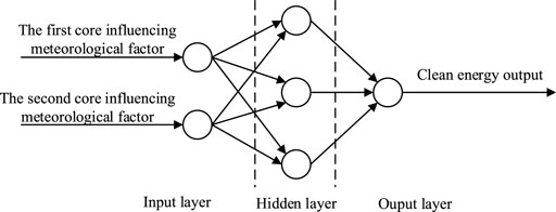
FIGURE 1. ANN model structure.

When ANN is used to fit the clean energy output and meteorological data, different variables in the original meteorological data usually have different units, and the order of magnitude also differs. According to the characteristics of neuron activation function, the output of neurons is usually limited to a certain range. Most nonlinear activation functions used in ANN are functions, and their output is limited to (0,1) or (−1,1). Directly fitting the input network with the original data will cause the neurons to saturate. Therefore, before using a neural network for fitting, the sample data with different dimensions must be normalized to eliminate the impact of the varying forms of original data. When the required input and target data fall into the (0,1) range, the normalization formula is given by

$p_t^{\ast }=\frac{p_t-p_{\min }}{p_{\max }-p_{\min }},(8)$

where $p_t$ represents the time data, and $p_{\max }$ and $p_{\min }$ represent the maximum and minimum values in the sequence to which the data belongs, which are the normalized data.

The neural network learning algorithm adopted by the ANN model is the Levenberg–Marquardt optimization method. The Levenberg–Marquardt optimization method can shorten the learning time and has a good effect in practical application (Zhang et al., 2021a). Its weight or threshold update formula is

$X_{k+1}=X_k-{\left(J^{T}J+uI\right)}^{-1}{J}^{T}e,(9)$

where j is the Jacobian matrix of the differential between the error and weight, e is the error vector, and u is a scalar.

After completing the training of ANN, the meteorological factors with the third highest relational degree are determined according to the GRA results. The historical data corresponding to the two meteorological factors with the highest relational degree are selected when the meteorological factors have a 90% maximum, 10% minimum, and median. After normalization, these values are used as the horizontal and vertical axes to represent the meteorological data on a grid. The meteorological data can cover all meteorological conditions despite the changing core meteorological factors of the analyzed power station. The gridded meteorological data are also used as the input of ANN, and the output of ANN is the gridded fitting results of clean energy output under different meteorological conditions. Then, a sensitivity analysis of the two core meteorological factors is conducted based on the fitting results. Finally, the quantitative relational between the multiple meteorological factors and clean energy output is obtained based on the variation trend and amplitude of clean energy output under varying core meteorological factors along with the influences of other meteorological factors.

3 Assessment method of development potential based on output prediction

The accurate prediction of the clean energy output is an important technique for handling the randomness, volatility, and intermittency of clean energy output. However, a day-ahead forecast entails high requirements for the continuity and integrity of historical data, and the input variable dimension of the forecast is high. This situation causes the model structure to be extremely complex and the prediction accuracy under varying weather conditions to be low. Therefore, the above association rules are used as the basis for identifying and optimizing the input variables. With this approach, the key influencing factors can be extracted, and the input set of the clean energy output prediction model can be built. However, the sample size of the data is insufficient. Therefore, the XGBoost algorithm is selected to predict the 24-hour day output of clean energy. The prediction results before and after the optimized selection of input variables are compared to verify the effectiveness of the screening input variables in relation to the relational analytical results. In addition, by constructing a fitting model without historical output data for determining the output of the new power station, the clean energy power fitting without historical output data can be more easily realized.

3.1 Clean energy output prediction based on XGBoost

XGBoost is an optimization boosting algorithm for integrating weak classifiers into a strong classifier (Zhang et al., 2021b). XGBoost generates a new tree via continuous iteration to fit the residual of the previous tree. As the iteration time increases, the accuracy continues to improve. Therefore, XGBoost can better fit the output data, and it can reduce the prediction error and achieve relatively high prediction accuracy The prediction model based on XGBoost is expressed as

${\widehat{y}}_i={\displaystyle \sum _{t=1}^n{f}_t\left(x_i\right),}{f}_t\in F,(10)$

where n is the number of trees, f_t is a function in function space F, ${\widehat{y}}_i$ is the predicted value of clean energy output, x_i is the ith data input, and F represents all possible cart sets. The tree model used in this research is the cart regression tree model.

Each iteration does not affect the model (i.e., the original model remains unchanged), and a new function is added to the model. One function corresponds to one tree. The newly generated tree fits the residual of the last prediction. The iterative process is given by

$\{\begin{array}{c}{\widehat{y}}_i^{\left(0\right)}=0\\ {\widehat{y}}_i^{\left(1\right)}=f_1\left(x_i\right)={\widehat{y}}_i^{\left(0\right)}+f_1\left(x_i\right)\\ {\widehat{y}}_i^{\left(t\right)}={\widehat{y}}_i^{\left(t-1\right)}+f_t\left(x_i\right)\end{array}.(11)$

The objective function of XGBoost is expressed as follows:

$X_{\text{obj}}={\displaystyle \sum _{i=1}^{n}l\left(y,\widehat{y}\right)}+{\displaystyle \sum _{k=1}^K\text{Ω}\left(f_k\right)},(12)$

$\text{Ω}\left(f_k\right)=\gamma T+\mathit{\lambda }\frac{1}{2}{\displaystyle \sum _{j=1}^T{\omega }_j^2},(13)$

where ${\displaystyle \sum _{i=1}^{n}l\left(y,\widehat{y}\right)}$ is used to measure the difference between the predicted output and the real output, ${\displaystyle \sum _{k=1}^K\Omega \left(f_k\right)}$ is a regularization term, T is the number of leaf nodes, and $\omega$ is the score of the leaf node. The purpose of $\gamma$ is to control the number of leaf nodes, and $\lambda$ is used to ensure that the score of leaf nodes is not extremely large. The goal of regularization is to select a simple prediction function to prevent the model from overfitting. When the regularization parameter is zero, XGBoost degenerates to the traditional boosting model. The iteration of the model adopts the method of additional training to further minimize the objective function (Xie et al., 2021). Then, the objective function is updated to

${\tau }^{\left(t\right)}={\displaystyle \sum _{i=1}^{n}l\left(y_i,{\widehat{y}}_i^{\left(t-1\right)}+f_t\left(X_i\right)\right)+\text{Ω}\left(f_t\right)}.(14)$

The Taylor series of the loss function is extended to the second order to find an approximation for minimizing the objective function using its Taylor second-order expansion at $f_t=0$. As such, the objective function is approximately

${\tau }^{\left(t\right)}\simeq {\displaystyle \sum _{i=1}^n\left[l\left(y_i,{\widehat{y}}_i^{\left(t-1\right)}+f_t\left(X_i\right)\right)+\frac{1}{2}{h}_i{f}_i^2\left(X_i\right)\right]+\text{Ω}\left(f_t\right)},(15)$

$\begin{array}{l}{X}_{\text{obj}}\simeq {\displaystyle \sum _{i=1}^n\left[g_i{f}_t\left(x_i\right))+\frac{1}{2}{h}_i{f}_t^2\left(x_i\right)\right]}+\text{Ω}\left(f_t\right)={\displaystyle \sum _{i=1}^n\left[g_i{w}_q\left(x_i\right))+\frac{1}{2}{h}_i{w}_q^2\left(x_i\right)\right]}+\text{Ω}\left(f_t\right)+\lambda T+\lambda \frac{1}{2}{\displaystyle \sum _{j=1}^T{\omega }_j^2}\\ ={\displaystyle \sum _{j=1}^T\left[\left({\displaystyle \sum _{i\in I_j}{g}_i}\right)w_j+\frac{1}{2}\left({\displaystyle \sum _{i\in I_j}{h}_i}+\mathit{\lambda }\right)w_j^2\right]}+\mathit{\lambda }T,\end{array}(16)$

where $X_{\text{obj}}$ is the objective function, $g_i=\partial {\widehat{y}}^{t-1}l\left(y_i,{\widehat{y}}^{t-1}\right)$ is the first derivative, and $h_i={\partial }^2{\widehat{y}}^{t-1}l\left(y_i,{\widehat{y}}^{t-1}\right)$ is the second derivative.

In the training process, the model continuously calculates the node loss to select the leaf node with the largest gain loss. Eq. 19 rewrites the objective function into a univariate quadratic function for the leaf node fraction $\omega$. The optimal $\omega$ and objective function values obtained from the solution are given by

${\omega }_j^{\ast }=-{\displaystyle \sum _{i\in I_j}{g}_i}/\left({\displaystyle \sum _{i\in I_j}{h}_i+\mathit{\lambda }}\right),(17)$

$X_{\text{obj}}=-\frac{1}{2}{\displaystyle \sum _{j=1}^T\frac{G_j}{H_j+\mathit{\lambda }}}+\mathit{\lambda }Tn.(18)$

The average absolute percentage error is selected as the main evaluation index of model prediction performance.

$X_{\text{MAPE}}=\frac{1}{n}{\displaystyle \sum _{t=1}^n\frac{\left|y_t-y_t^{\text{Ω}}\right|}{y_t}}\ast 100\%(19)$

3.2 Development potential assessment index of regional clean energy stations

The regional potential index that considers the spatial–temporal characteristics of clean energy output (i.e., guaranteed output coefficient (GOC), maximum output coefficient (MOC), and effective capacity coefficient) is proposed in this study. The assessment of clean energy stations can greatly help to alleviate the contradiction between the continuous increase in the installed capacity of clean energy and the shortage of delivery channels and transmission capacity. Clean energy power generation is developing rapidly, but a large number of clean energy systems are located in areas with weak power grids or even have no electricity. The distribution of clean energy resources is situated far away from load centers. Thus, clean energy, including decentralized wind power access and distributed photovoltaic power generation, is difficult to absorb and utilize, consequently facing the problem of limited transmission. Moreover, the output of each regional clean energy station is affected by its inherent randomness, volatility, and intermittency, and the output of each station is complementary. Therefore, simply adding maximum capacity should be abandoned as an idea when evaluating clean energy access and its transmission scheme; otherwise, serious economic losses may arise at the beginning of the station system design. A suitable approach is to classify clean energy stations by region, aggregate and analyze the output of each station, and build a reasonable evaluation framework for the access and transmission planning scheme of these clean energy stations.

Take wind power as an example, and rank the annual hourly output of wind farms from large to small (except for zero). As shown in Figure 2, its monotonic decline curve can depict the probability in which the wind power output is higher (or lower) than a certain value.

1) 95% MOC represents the percentage of maximum instantaneous output corresponding to the 95% guarantee rate of the installed capacity of the statistical power generation output value that is greater than the 95% guarantee rate. This parameter can characterize the high-value characteristics of clean energy output.

2) The GOC of wind power guaranteed output represents the probability in which the wind power output is greater than the wind power output at all times (i.e., 95%).

3) Available capacity coefficient (AVC) refers to the percentage of maximum output of the clean energy power stations corresponding to part of the accumulated electricity in the installed capacity under a 95% wind rejection rate. This parameter can help to guide the planning of access and transmission capacity of regional clean energy power stations.

$X_{\text{AVC,all}}={\displaystyle \sum _{t=t_{95\text{,avc}}}^n{p}_{t,n}}/P_n\ast 100\%,(20)$

where $t_{95\text{,avc}}$ is the cumulative time when the air rejection rate is 95%, and $P_n$ is the installed capacity of wind power station n.

FIGURE 2

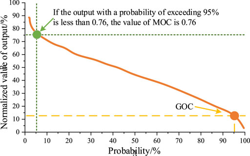
FIGURE 2. Output characteristic index of the wind power station.

The specific framework of the assessment method for the development potential of regional clean energy bases is shown in Figure 3. First, the historical data are integrated to obtain the output meteorological factor dataset of a single station. The meteorological factors with a core influence are obtained according to GRA, and the single-factor relational analytical results are derived. Then, ANN is used to fit the historical data and core meteorological factors, and sensitivity analysis is performed to obtain the results of multi-factor coupling relational analysis. Take the above relational results as the basis for identifying and optimizing input variables to extract the key influencing factors and build the input set of clean energy output prediction models. XGBoost is selected to predict the clean energy output 24 h before the day. The prediction results before and after the optimized selection of input variables are compared to verify the effectiveness of the screening input variables in relation to the relational analytical results. By constructing a fitting model without historical output data for determining the output of the new power station, the clean energy power fitting without historical output data can be realized. Finally, the development potential indicators (GOC, MOC, and AOC) of the regional clean energy station are calculated.

FIGURE 3

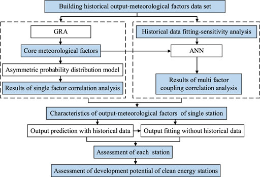
FIGURE 3. Framework of the development potential assessment method of regional clean energy stations.

4 Case study

A wind power station in regional #A is initially selected to analyze the correlation between the output and meteorological factors, and the output is predicted based on this approach. Then, several stations in the region are predicted, and the development potential of the regional clean energy base is evaluated. The output characteristics of the #A wind power stations in 2019 and 2020 are shown in Figure 4.

FIGURE 4

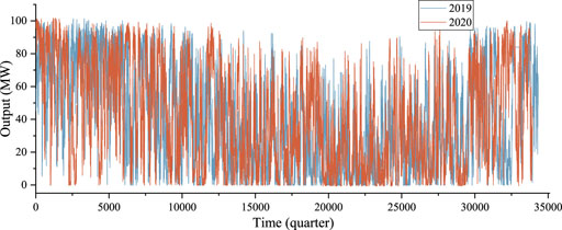
FIGURE 4. Output characteristics of wind station #A in 2019 and 2020.

4.1 Relational analysis of the output and meteorological factors

Meteorological factors, such as wind speed, wind direction, temperature, humidity, and air pressure, are selected to analyze the relational among wet season, dry season, and normal season. The results are shown in Table 1.

TABLE 1

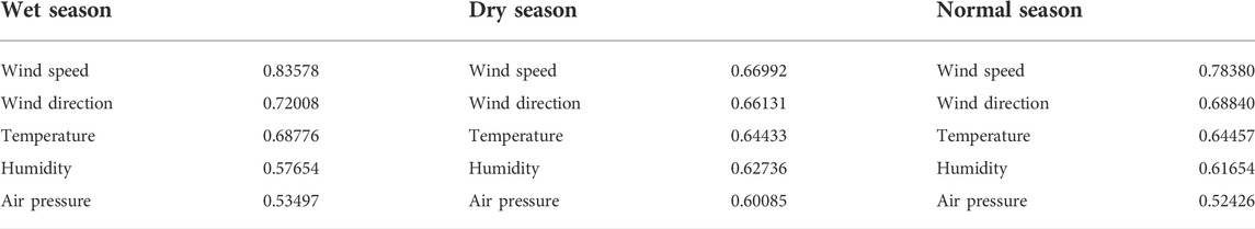
TABLE 1. Relational analysis of core meteorological factors of the wind power station.

Given the relatively open environment, the wind direction of the wind power station is variable. At this time, wind direction is the dominant factor as opposed to wind speed, and humidity and relative temperature are the dominant factors. A review of the historical data in 2019–2020 indicates a gradual weakening of monsoon intensity, but the impact of the southeast monsoon is increasing. The wind direction is affected by the southwest monsoon, northwest monsoon, and southeast monsoon, and it changes greatly. On the one hand, the cross-influence of various monsoons brings changes to wind speed and wind direction; on the other hand, it greatly affects air humidity. Therefore, the influence of humidity on wind power is significantly increased in the dry season. The increase in the correlation among wind direction, humidity, and wind power during the dry season for the wind power plant is fundamentally caused by the cross-influence of the southwest monsoon and southeast monsoon in winter. Wind direction and humidity are the concrete representations of the interaction of the monsoon.

4.2 Relational analysis of multiple factors

After completing the ANN training, the meteorological factors with the third highest relational degree are determined in relation to the results of GRA. The historical data corresponding to the two meteorological factors with the highest relational degree are selected when the meteorological factors have a 90% maximum, 10% minimum, and median. After normalization, the data are used as the horizontal and vertical axes to represent the meteorological data on a grid. The meteorological data can cover all meteorological conditions despite the varying core meteorological factors of the analyzed power station. The gridded meteorological data are also used as the input of the neural network, and the output of the neural network is the gridded fitting results of clean energy output under different meteorological conditions. Then, a sensitivity analysis of the two core meteorological factors is performed based on the fitting results. Finally, the quantitative relational between the multiple meteorological factors and clean energy output is obtained based on the variation trend and amplitude of clean energy output under varying core meteorological factors that change along with the influences of other meteorological factors.

The #A wind speed temperature wind power distribution diagram of the wind power station under different wind directions across periods (wet season and normal season) is shown in Figure 5.

FIGURE 5

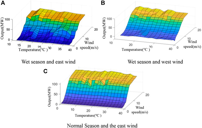
FIGURE 5. Wind speed–temperature–output distribution diagram of the wind power station across periods under different wind directions. (A) Wet season and east wind. (B) Wet season and west wind. (C) Normal Season and the east wind.

The output change of the wind power station is less sensitive to temperature during the wet and normal periods, and the temperature change hardly affects the wind speed wind power conversion curve. Under the same wind speed but different temperature conditions, the output of the wind power plant does not change significantly. In the dry season, the output of the wind power plant is affected by multiple monsoons. At this time, the wind turbine may be frequently cut off, and other control phenomena (i.e., the change in wind speed is not proportional to wind power) may arise. The correlation uncertainty between wind speed and wind power is extremely strong.

4.3 Wind power output forecast based on XGBoost

The effect of input variable selection, which is based on association rule optimization, on prediction performance and the effectiveness of the output prediction of clean energy are compared using the XGBoost prediction model of the original input variables. After filtering the input variables, the long-term short-term memory (LSTM) ANN and deep belief network (DBN) are constructed for the 24-hour short-term WPF. In the short-term WPF model, the initial learning rate of the constructed XGBoost model is set to 0.01, the maximum number of iterations is set to 300, the maximum depth of the tree is set to 6, and the loss function is set to linear regression. The results are shown in Figure 6.

FIGURE 6

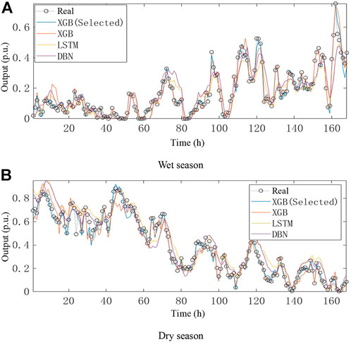
FIGURE 6. Comparison of output prediction results of the different algorithms. (A) Wet season. (B) Dry season.

Figure 6 shows the general trend of the overall prediction accuracy of LSTM and DBN. The prediction deviation is large at different times. The XGBoost model has a better fitting accuracy on the actual output, and the variation law of the prediction result is consistent with the actual data. Especially in the time period of rapid wind power fluctuation, the prediction effect of XGBoost is significantly better than the other two algorithms. Compared with the XGBoost with the post-screened input variables, the XGBoost model with the original data used as the input variables has the characteristics of overfitting, and the prediction results are obviously deviated from the actual data.

Then, the wind power’s normalized mean absolute error (MAE) prediction error and the prediction accuracy (based on the root mean square error) of the XGBoost model before and after optimally selecting the input variables in relation to the association rules are calculated. The LSTM and DBN are also computed using the test set after optimally selecting the input variables. The results are shown in Tables 2, 3.

TABLE 2

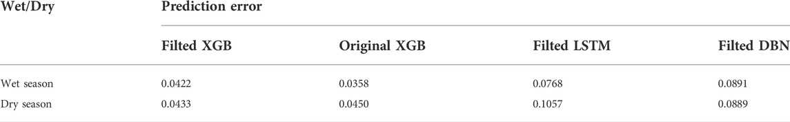
TABLE 2. Prediction error of wind power.

TABLE 3

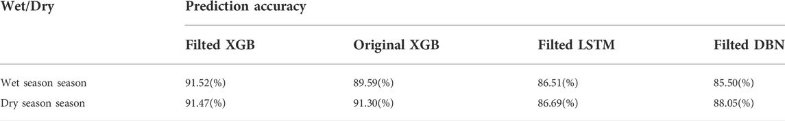
TABLE 3. Prediction accuracy of wind power.

The results, combined with the trends in Figure 6, indicate that the dimension reduction measures based on the correlation characteristics can reduce the complexity of the prediction model, effectively improve the prediction effect of XGBoost, and screen the input variables to reduce the impact of randomness and intermittency of wind power on the final results of the prediction model. The measures are applicable for solving the problem of unstable accuracy of the prediction model in cases of rapid and large-scale fluctuations of wind power.

4.4 Output fitting without historical energy data

XGBoost is also used to build the wind power fitting model without historical energy data. The validity of the fitting model is verified by comparing the results of the wind power fitting model with historical energy data. The comparison between the actual wind power and fitting results is shown in Figure 7.

FIGURE 7

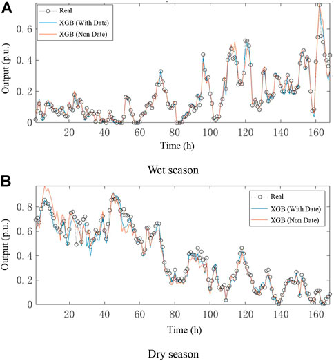
FIGURE 7. Fitted prediction of wind power output. (A) Wet season. (B) Dry season

According to Figure 7, under the condition of small wind power and stable change, the overall accuracy of the wind power fitting model without historical energy data is high. In particular, as shown in Figure 7A, the fitting results coincide with the actual data within the time of 1–100, which can well depict the output of wind power. When the meteorological factors change violently with the weather conditions, the wind power also fluctuates greatly, and the frequency is high. Furthermore, the deviation between the fitting results and the actual data under this condition increases to a certain extent compared with those under conventional weather, but the deviation can still approximate the variation of wind power. Similarly, as shown in Figure 7B, within the time of 155–162, the fitting results accurately depict a steep drop and increase in actual wind power, and the maximum and minimum points of both scenarios are the same.

The accuracy of WPF/fitting based on RMSE is shown in Table 4.

TABLE 4

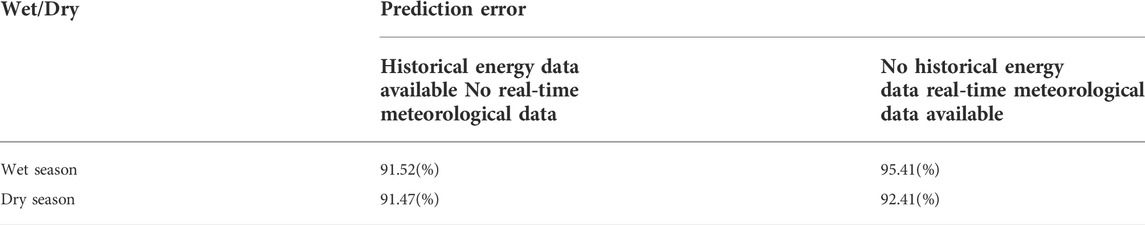
TABLE 4. Fitted prediction error of wind power.

Although the use of historical output data is less effective than the day-ahead prediction model, the results of the fitting model without the historical output data are consistent with the actual data for most time periods owing to the integration of real-time meteorological information. Moreover, the prediction error value is within a good range, and the fitting effect on the variation trend of wind power is better under complex and changeable meteorological conditions. However, when the meteorological data changes abruptly and the overall fitting error is extremely large, the fitting result with the historical energy data is better.

4.5 Assessment of the wind power station

The total installed capacities of the wind power base in 2019 and 2020 were 1669 and 2166 MW, respectively. The hourly output data of wind power for 2019 and 2020 are sorted from large to small, and the results are shown in Figures 8, 9, respectively. The AOC of wind power corresponding to the key effective capacity for 2019 and 2020 are shown in Tables 5, 6.

FIGURE 8

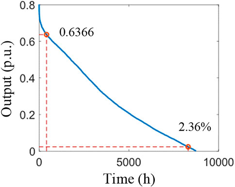
FIGURE 8. Descending order of hourly output in 2019.

FIGURE 9

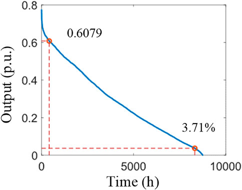
FIGURE 9. Descending order of hourly output in 2020.

TABLE 5

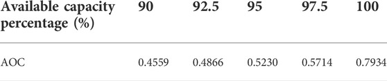
TABLE 5. AOC of wind power corresponding to key AOC in 2019.

TABLE 6

TABLE 6. AOC of wind power corresponding to key AOC in 2020.

The comparative trends in the 2019 and 2020 output descending charts with the effective capacity coefficient show a significantly lower value for 95% MOC in 2020 compared with that in 2019. On the one hand, the overall output of the wind power plants that have been newly added to the assessment in 2020 is low, thereby increasing the low output of the wind power hourly output in 2020. On the other hand, the overall distribution of the effective capacity coefficient of this wind power base in 2020 has also decreased with respect to the previous 2 years, but the surge trend of the effective capacity coefficient within the range of effective capacity percentage greater than 97.5% is still significant.

4.6 Development potential assessment for the wind power stations

This study proposes the construction of 12 new wind power stations in the wind power base based on the assumption that the installed capacity is 200 MW. At this phase of this study, the power stations are stacked for further analysis. The total installed capacity of the wind power base in 2020 was 2166.2 MW. Subsequently, 600 and 2200 MW are added to this total installed capacity for the assessment are shown in Figures 10, 11 respectively.

FIGURE 10

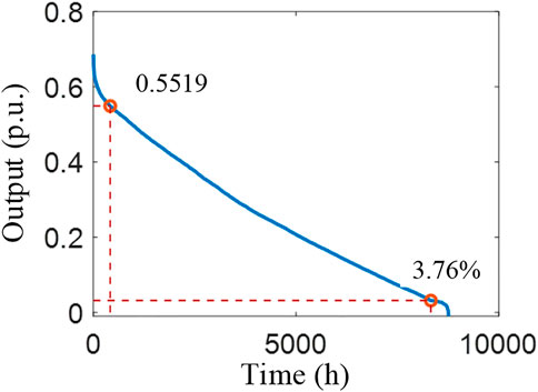
FIGURE 10. Descending order of hourly output (600 MW).

FIGURE 11

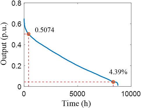
FIGURE 11. Descending order of hourly output (2200 MW).

The AOC of the wind power stations corresponding to the key effective capacity of the wind power base (increased by 600 and 2200 MW) is shown in Tables 7, 8. In addition, Figure 12 shows the AOC of the wind power base and the total installed capacity of regional wind power stations.

TABLE 7

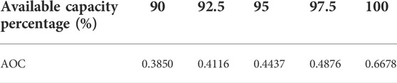
TABLE 7. AOC of wind power corresponding to key AOC (600 MW).

TABLE 8

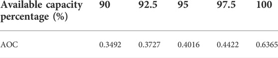
TABLE 8. AOC of wind power corresponding to key AOC (2200 MW).

FIGURE 12

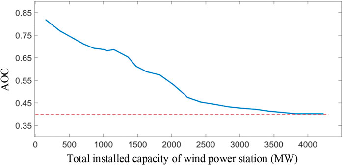
FIGURE 12. AOC of regional wind power stations with different total regional installed capacity.

The AOC of the regional wind power stations with different total regional installed capacities is also shown in Figure 12.

Figure 12 shows that as the number of power stations continues to increase, the total installed capacity of the wind power base continues to rise, and the effective capacity factor continues to decrease. However, when the total installed capacity is higher than 3500 MW, the effective capacity factor remains around 0.4. Thus, given the existing meteorological data, when the number of wind power stations is increased to a certain extent, the total wind power output characteristics in the region will not change significantly. This finding is consistent with the inherent randomness of wind power.

5 Conclusion

This study presents a development potential assessment method for clean energy stations. First, the relational between the clean energy output and meteorological factors is investigated via GRA and ANN fitting. Second, XGBoost-based relational analysis is used to predict 24 h of clean energy output by referring to historical data, and then the output of the power stations is fitted without using historical data. Finally, the AVC, GOC, and MOC of wind power for future clean energy stations are calculated to guide the planning of regional stations. The findings indicate that new clean energy stations will significantly affect the MOC, GOC, and AVC of wind power. When the number of new stations and the overall installed capacity of the region are both increased, the AOC and MOC of the regional wind power stations will gradually decrease, whereas the GOC will gradually increase. Cases of regional wind power stations are also analyzed in this work. The analytical results prove that the proposed method is effective and has strong applicability.

Data availability statement

The original contributions presented in the study are included in the article/supplementary material, further inquiries can be directed to the corresponding author.

Author Contributions

WC and JD: writing—original draft preparation. GW, TL, and WX: conceptualization and funding acquisition. YX: supervision and revise the paper.

Conflict of interest

The authors declare that the research was conducted in the absence of any commercial or financial relationships that could be construed as a potential conflict of interest.

Publisher’s note

All claims expressed in this article are solely those of the authors and do not necessarily represent those of their affiliated organizations, or those of the publisher, the editors and the reviewers. Any product that may be evaluated in this article, or claim that may be made by its manufacturer, is not guaranteed or endorsed by the publisher.

References

An, J., Yin, F., Wu, M., She, J., and Chen, X. (2021). Multisource wind speed fusion method for short-term wind power prediction. IEEE Trans. Ind. Inf. 17 (9), 5927–5937. doi:10.1109/tii.2020.3006928

CrossRef Full Text | Google Scholar

He, B., Ye, L., Pei, M., Lu, P., Dai, B., Li, Z., et al. (2022). A combined model for short-term wind power forecasting based on the analysis of numerical weather prediction data. Energy Rep. 8, 929–939. doi:10.1016/j.egyr.2021.10.102

CrossRef Full Text | Google Scholar

Jiahao, Ye, Xia, Wei, and Huang, Deqi (2022). Short-term forecast of wind power based on bso-elm-adaboost with grey correlation analysis. Acta Energiae Solaris Sin. 43 (3), 426–432.

Google Scholar

Kanwal, S., Khan, B., and Rauf, M. Q. (2020). Infrastructure of sustainable energy development in Pakistan: A review. J. Mod. Power Syst. Clean Energy 8 (2), 206–218. doi:10.35833/mpce.2019.000252

CrossRef Full Text | Google Scholar

Li, C., Wang, N., Shen, X., Zhang, Y., Yang, Z., Tong, X., et al. (2022). Energy planning of Beijing towards low-carbon, clean and efficient development in 2035. CSEE J. Power Energy Syst.

Google Scholar

Li, M., Yang, M., Yu, Y., and Lee, W. J. (2022). A wind speed correction method based on modified hidden markov model for enhancing wind power forecast. IEEE Trans. Ind. Appl. 58 (1), 656–666. doi:10.1109/tia.2021.3127145

CrossRef Full Text | Google Scholar

Liu, C., Zhang, X., Mei, S., Zhen, Z., Jia, M., Li, Z., et al. (2022). Numerical weather prediction enhanced wind power forecasting: Rank ensemble and probabilistic fluctuation awareness. Appl. Energy 313, 118769. doi:10.1016/j.apenergy.2022.118769

CrossRef Full Text | Google Scholar

Momete, D. C. (2018). Analysis of the potential of clean energy deployment in the European union. IEEE Access 6, 54811–54822. doi:10.1109/access.2018.2872786

CrossRef Full Text | Google Scholar

Ogliari, E., Guilizzoni, M., Giglio, A., and Pretto, S. (2021). Wind power 24-h ahead forecast by an artificial neural network and an hybrid model: Comparison of the predictive performance. Renew. Energy 178, 1466–1474. doi:10.1016/j.renene.2021.06.108

CrossRef Full Text | Google Scholar

Ozkan, M. B., and Karagoz, P. (2019). Data mining-based upscaling approach for regional wind power forecasting: Regional statistical hybrid wind power forecast technique (RegionalSHWIP). IEEE Access 7, 171790–171800. doi:10.1109/access.2019.2956203

CrossRef Full Text | Google Scholar

Sanjari, M. J., Gooi, H. B., and Nair, N. C. (2020). Power generation forecast of hybrid PV–wind system. IEEE Trans. Sustain. Energy 11 (2), 703–712. doi:10.1109/tste.2019.2903900

CrossRef Full Text | Google Scholar

Shi, J., Ding, Z., Lee, W., Yang, Y., Liu, Y., Zhang, M., et al. (2014). Hybrid forecasting model for very-short term wind power forecasting based on grey relational analysis and wind speed distribution features. IEEE Trans. Smart Grid 5 (1), 521–526. doi:10.1109/tsg.2013.2283269

CrossRef Full Text | Google Scholar

Taylor, J. W., McSharry, P. E., and Buizza, R. (2009). Wind power density forecasting using ensemble predictions and time series models. IEEE Trans. Energy Convers. 24 (3), 775–782. doi:10.1109/tec.2009.2025431

CrossRef Full Text | Google Scholar

Vladislavleva, E., Friedrich, T., Neumann, F., and Wagner, M. (2013). Predicting the energy output of wind farms based on weather data: Important variables and their correlation. Renew. Energy 50, 236–243. doi:10.1016/j.renene.2012.06.036

CrossRef Full Text | Google Scholar

Wan, J., Wang, Q., and Chan, A. B. (2022). Kernel-based density map generation for dense object counting. IEEE Trans. Pattern Anal. Mach. Intell. 44 (3), 1357–1370. doi:10.1109/tpami.2020.3022878

PubMed Abstract | CrossRef Full Text | Google Scholar

Wang, Yanliang, and Yue, Xiang (2022). Photovoltaic-storage energy system management considering wireless data communication. Energy Rep. 8, 267–273. doi:10.1016/j.egyr.2022.05.152

CrossRef Full Text | Google Scholar

Wang, Z., Zhang, J., Zhang, Y., Huang, C., and Wang, L. (2020). Short-term wind speed forecasting based on information of neighboring wind farms. IEEE Access 8, 16760–16770. doi:10.1109/access.2020.2966268

CrossRef Full Text | Google Scholar

Wei, X., Yue, X., Li, J., and Liu, J. (2022). Wind power bidding coordinated with energy storage system operation in real-time electricity market: A maximum entropy deep reinforcement learning approach. Energy Rep. 8, 770–775. doi:10.1016/j.egyr.2021.11.216

CrossRef Full Text | Google Scholar

Wu, Y. -K., Wu, Y. -C., Hong, J. -S., Phan, L. H., and Phan, Q. D. (2021). Probabilistic forecast of wind power generation with data processing and numerical weather predictions. IEEE Trans. Ind. Appl. 57 (1), 36–45. doi:10.1109/tia.2020.3037264

CrossRef Full Text | Google Scholar

Xiang, Y., Liu, J., Hu, S., and Wang, R. (2021). An improved fuzzy method for characterizing wind power. J. Mod. Power Syst. Clean Energy 9 (2), 459–462. doi:10.35833/mpce.2020.000169

CrossRef Full Text | Google Scholar

Xie, J., Li, Z., Zhou, Z., and Liu, S. (2021). A novel bearing fault classification method based on XGBoost: The fusion of deep learning-based features and empirical features. IEEE Trans. Instrum. Meas. 70, 1–9. doi:10.1109/tim.2020.3042315

PubMed Abstract | CrossRef Full Text | Google Scholar

Zhang, G., Xia, B., and Wang, J. (2021). Intelligent state of charge estimation of lithium-ion batteries based on L-M optimized back-propagation neural network. J. Energy Storage 44 (Part B), 103442. doi:10.1016/j.est.2021.103442

CrossRef Full Text | Google Scholar

Zhang, S., Zhang, D., Qiao, J., Wang, X., and Zhang, Z. (2021). Preventive control for power system transient security based on XGBoost and DC OPF with consideration of model interpretability. CSEE J. Power Energy Syst. 7 (2), 279–294.

Google Scholar