A secure edge power system based on a Docker container

Thanks to the advantages of low latency, high efficiency, and oneself-security, the edge computing (EC) paradigm is expected to widely be applied in a large number of scenarios. However, because EC equipment is closer to a wide variety of terminals in a realistic environment, it is also more vulnerable to terminal attacks. The security of edge computing equipment itself cannot be ignored. Docker is a lightweight container technology that closely fits the existing needs of edge computing for portability, security isolation, and convenience. In this paper, Docker technology is taken as an edge computing security support engine and a security monitoring system based on the Docker container is built. In addition, combined with container monitoring and objective weighting method, a node security judgment method is proposed. Finally, according to the results of the node security judgment, a method for evaluating the security of the unmonitored node is put forward. Consequently, an edge computing security monitoring system based on the Docker container is built, and its performance in the real environment of a smart grid system is implemented to verify the proposed method. The results prove the efficiency and security protection of the novel edge power system.

1 Introduction

Edge computing refers to the technology of computing on the edge of a network. An edge is defined as any computing and network resource node between the data source and data center (Taleb et al., 2017). Edge computing has attracted extensive attention because of its low delay, security, and lightweight (Song et al., 2021a) and it has been applied to smart cities, smart grids, the Internet of vehicles, the Internet of Things, and many other fields (Liu et al., 2018).

However, edge computing also faces some security problems (Muñoz et al., 2018). At the beginning of the development of edge computing, the idea of security first was put forward to avoid the passive security remedy of “patching.” (ECC, 2016; ECC and AII, 2019). For example, under industry Internet of Things (IIoT) scenarios, the introduction of more information equipment in the industrial scene also indirectly introduces new security risks and provides new attack methods for criminals (AII, 2018). Edge computing devices are also vulnerable to terminal attacks because they are close to the terminal (Neshenko et al., 2019). In particular, edge computing faces multiple attacks, such as multiple terminal access, heterogeneous data storage (Kushida and Pingali, 2014), and different application running programs, which requires edge computing devices to provide various forms of security protection for the terminal data and applications running on them (Song et al., 2021b); for example, secure transmission protection, terminal access authentication, data storage, application protection on edge devices, and so on (Song et al., 2022). All of these security protection issues need a secure edge computing support engine.

Docker technology is a container technology that is based on the concept of a “sandbox,” which has the advantages of lightweight, convenience, and security isolation (Reis et al., 2022). It first appeared in 2013 as an open-source cloud project that was based on the Go language implemented by GitHub. The main workflow of Docker is shown in Figure 1. According to the user’s requirements, the Docker registry distributes the Docker image to the local host (Zhao et al., 2021). The local host then builds Docker containers of different systems through kernel reuse based on the “sandbox” mechanism (Liu et al., 2020). Docker’s kernel reuse function provides a unified operation specification for multiple operating systems and applications developed in different languages. Different programs can run on any host installed with the Docker engine, requiring only the unified Docker encapsulation. By encapsulating the environment and packaging dependently, multiple independent system container environments can be provided on a single operating system (Rabay’a et al., 2019). Docker uses Linux underlying functions (e.g., the Namespace component and Control groups component) to isolate containers, processes, and systems from each other, which is the best counterpart of the EC security requirement (Yadav et al., 2018).

FIGURE 1

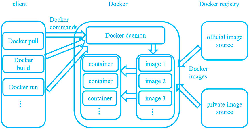
FIGURE 1. The workflow of Docker.

The lightweight, security, and isolation advantages of the Docker have led to a large number of research efforts (Cai et al., 2019). For example, an emergency communication system response to natural disasters has been established using Docker and Rsync utility, making use of the lightweight and rapid deployment characteristics of Docker to reduce the use of system resources (Kumar Pentyala et al., 2017). Agarwal (2022) designed a user-friendly interface for inspecting, interacting with, and managing Docker objects, such as containers and Docker Compose-based applications to quickly install a fusion experiment data storage and management system (JCDB). Liu et al. (2018) used Docker to automatically deploy standardized cloud databases and Web applications. Docker’s image deployment function has also been studied. For example, Smet et al. (2018) proposed an on-demand deployment scheme using the Docker platform to realize the optimal allocation of resources under the micro service architecture. Meanwhile, Kwon and Lee (2020) designed a Docker Image Vulnerability Diagnostic System (DIVDS) for a reliable Docker environment in their article. This system can diagnose uploading or downloading Docker images to judge security. Abhishek and Rajeswara (2021). focus on the security of the Docker container and proposed a framework that uses an architecture including plugins, and a CI/CD pipeline to deploy the application to ensure the security of the application bundled as a Docker image. Şengül (2021) focused on the Docker container and the security issues of the Docker reuse host kernel, and proposed a method including static and dynamic analysis to ensure Docker image and container security. Rahmansyah et al. (2021) focused on the security of the Docker daemon. and found a way to reduce the Docker daemon attack surface by using rootless mode.

The Docker container on the host node in the edge computing model still lacks a comprehensive assessment. The application of Docker technology also faces some problems. First, can we find a way to make full use of the security of Docker container with low consumption? Second, when Docker is applied to nodes as a security engine, can developers judge the security of host nodes through the security of Docker containers? Finally, when some nodes in the edge network deploy Docker containers, how can we evaluate the security of other nodes without Docker containers? To solve these three problems, this article first provides a paradigm for Docker application under edge computing and designs a three-layer container monitoring model based on container monitoring software to improve the security performance of Docker. Based on the results of the Docker container monitoring model, we propose a novel scheme to judge node security with the objective weighting method. Finally, based on the idea of community division and PageRank algorithm, a new security evaluation scheme for those nodes without monitoring is proposed.

The rest of this paper is organized as follows. Section 2 proposes an application paradigm of Docker container under the edge computing model and the three-layer monitoring model. The security judgment scheme of the monitored nodes is introduced in Section 3. Section 4 provides a security evaluation scheme for the unmonitored nodes. Experiments and results are presented in Section 5. Finally, Section 6 concludes this paper.

2 System model

This study presents an application paradigm of the Docker container under the edge computing model. As shown in Figure 2, the model’s architecture is divided into three layers: cloud, edge, and terminal. The cloud server has cloud computing, data storage, resource sharing, and other functions to interact with edge computing devices and issue control instructions (Vaishnav, 2021). The Docker container can be regarded as the “security support engine” of the operating system. Databases, control programs, and other applications on edge computing devices can be run in isolation by Dockers. The user’s programs on terminal devices are also isolated using Docker containers to ensure their security. At the same time, the model needs to build an external private Docker container image registry. The registry issues different images according to the needs of edge computing devices and the user’s need to build Docker containers with different functions.

FIGURE 2

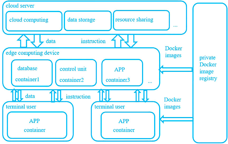
FIGURE 2. The edge computing model based on Docker.

A Docker container has certain security risks. Therefore, this article uses the container security monitoring software Prometheus to monitor the running states of the Docker container and judge its security. Although the container monitoring system cannot fundamentally solve the risk of a Docker container based on the Linux system, the monitoring software can monitor the operation status of the container in real-time and give a risk alarm to the container with abnormal operation according to the specified method (Zou et al., 2022). This provides a certain degree of security enhancement for a Docker container. We will next introduce the Prometheus monitoring software.

Prometheus is an open-source project that was developed in the Go language. Its working principle is to read the status of monitoring components and display them visually. The workflow of Prometheus is shown in Figure 3. Prometheus can capture the status of monitored components through HTTP protocol. Prometheus has high scalability because it can connect external components through HTTP. It also has many other advantages, including support for flexible query language, single node works independently, data can be stored in a time series database, and it has support for chart visualization interface configuration. The specific workflow of Prometheus is shown in Figure 3. Prometheus includes five core components, as follows: Server, Exporter, Alertmanager, Pushgateway, and Web UI. The main function of the Server component is to collect and store monitoring data. The data collected by Server component can also be queried through PromQL database language; The Alertmanager component is used to realize the alarm function. The user determines the monitoring threshold of the container or host by modifying the underlying YML file. When a monitoring indicator exceeds the threshold set in the alarm rules, the user can send alarm information to the monitor by email or other means. Pushgateway is used to collect the data cache of temporary nodes. When some nodes do not exist for a long time, the Prometheus server cannot grab the data. Pushgateway can push the indicators to the gateway for cache and upload them together when other indicators are collected. The main function of the Exporters is to report monitoring data to the server component.

FIGURE 3

FIGURE 3. The workflow of the Prometheus.

To improve the security of the edge computing model when Docker is applied to the edge computing model, we designed a three-layer container monitoring model based on the container monitoring software Prometheus. The architecture of the edge computing model can mainly be divided into three layers: cloud layer, edge computing layer, and terminal layer. Thus, the deployment of the monitoring system under edge computing should also be divided into three layers according to the architecture of the edge computing system. Specifically, it is realized through three parts: cloud monitoring, edge self-monitoring, and edge self-monitoring. According to the traditional node monitoring system and edge computing network system architecture, this paper constructs a three-tier container risk monitoring model from cloud to edge and then to user, as shown in Figure 4.

FIGURE 4

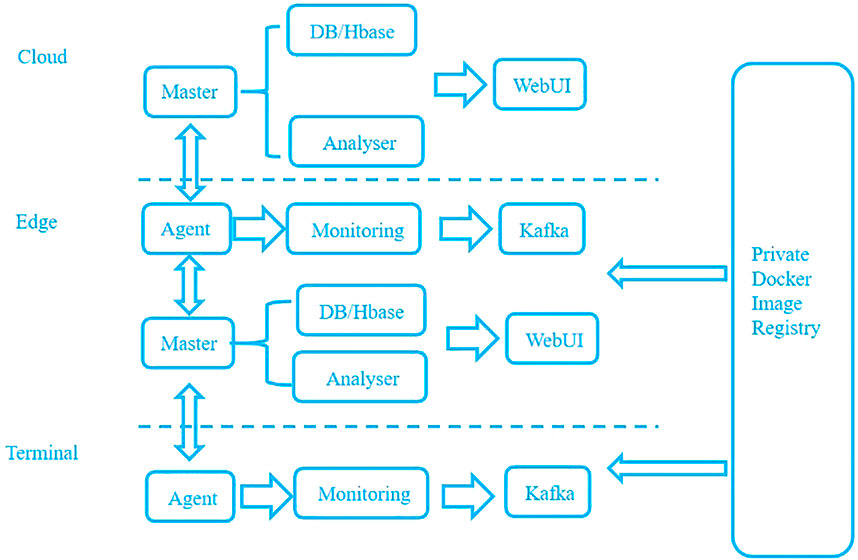
FIGURE 4. The architecture of three-layer container monitoring model.

As the general control unit of the monitoring model, Prometheus software should be deployed on the cloud server to monitor the edge computing node and collect the real-time monitoring data of the Docker container on the edge computing node. For Docker containers with abnormal monitoring indicators, the cloud server needs to take corresponding response measures (e.g., temporarily stopping the cloud service until the container indicators return to normal). For a container with an abnormal time that is too long or with too many alarms, the cloud can determine that the container is in a risk state, issue an instruction to delete the container, and then pull the image from the private Docker image registry to recreate the container.

After the Prometheus software is deployed on the cloud server, it integrates the functions of the master, DB/Hbase and analyzer. Prometheus software can realize the visual data display function of the web module by connecting with Grafana software. Prometheus software completes the task that the master module sends monitoring items from the cloud to the edge node through the Prometheus server component, pulls the monitoring indicator information of the edge node and passes it to the Pushgateway component, and then generates the data format that Prometheus software can recognize and display. The Prometheus server component stores the data and completes the data storage of DB/HBase module. The administrator configures the monitoring rules by configuring the YML file of the Prometheus monitoring software to build the monitoring model, configure the monitoring indicators of the Alertmanager component to realize the alarm function, and complete the alarm analysis of the analyzer module.

The edge computing node needs to upload its own container monitoring indicators upward and collect client container monitoring data downward. At the same time, the edge computing node also needs to have certain management authority over the container. When the cloud sends an instruction, the edge computing node should stop adding and deleting the container according to the command sent by the cloud. The total function of the edge side is divided into two parts: providing monitoring data to the cloud and monitoring the terminal container.

3 Security judgment scheme of the monitored node

After deploying the Docker and Prometheus software on the node of edge computing system, new problems have emerged. In particular, how should developers use Docker monitoring data to judge the running state of the container and then judge the security of the node? In this section, a novel security judgment scheme of monitoring nodes based on the K-means clustering algorithm and objective weighting method are proposed. The basic theory used in the scheme will be introduced in Section 3.1. The specific steps of the new scheme will be described in Section 3.2.

3.1 Theory

3.1.1 K-means

The K-means algorithm is used to determine the monitoring indicator threshold in this method. It is a kind of unsupervised learning algorithm that is commonly used in machine learning. The principle is to select a division method to make the similarity between clusters as small as possible and the similarity of nodes within clusters as large as possible through a given sample set and clusters to be divided (Esteves et al., 2013). Under a given data sample set $\mathrm{C}=\left\{X_1,X_2,\dots ,X_j,\dots ;X_j=\left(x_{j1},x_{j2},\dots ,x_{jd}\right)ϵR^d\right\}$, $X_j$ represents a sample value, usually in the form of a vector. Partition clustering divides the data into K clusters. Cluster partition needs to meet the following conditions:

$\{\begin{array}{c}C=\left\{C_1,C_2,\dots ,C_k\right\};K\le N\\ C_i\ne \varnothing ;i=\mathrm{1,2},\dots ,K\\ C_i\cap C_j=\varnothing ;i,j=\mathrm{1,2},\dots ,K,i\ne j\end{array}(1)$

Euclidean distance is usually used as an indicator to measure the similarity between data nodes. The calculation formula of Euclidean distance is as follows:

$\mathrm{d}\left(\mathrm{x},C_i\right)=\sqrt{{\displaystyle \sum }_{j=1}^m{\left(x_i-C_{ii}\right)}^2}(2)$

where x is the data sample, m is the dimension of the sample data, $C_i$ is the i-th cluster center, and $C_{ij}$ is the value of the j-th dimension of the i-th cluster center. The algorithm initially selects a cluster center, it then computes the Euclidean distance between each node and the cluster center, judges the data closest to the cluster center, and divides it into the same cluster (Kumar and Dhiman., 2021). Afterward it calculates the average value of all data in the same cluster and takes it as a new cluster center, and continuously iterates the above steps to update the position of the cluster center to reduce the error square sum SSE of the cluster (Chatterjee, 2021). The computing formula of the sum of squares of errors in the cluster SSE is as follows:

$\text{SSE}={\displaystyle \sum }_{x\in C_i}{\left|d\left(x,C_i\right)\right|}^2(3)$

After each iteration, judging whether the clustering center remains unchanged or whether the maximum number of iterations is reached. When these conditions are met, the algorithm is terminated.

3.1.2 Objective weighting method

3.1.2.1 Entropy weight method

Entropy is a physical quantity that is used to describe the degree of chaos within a system. The greater the entropy, the higher the degree of chaos; and the smaller the entropy, the lower the degree of chaos. The basic idea of the entropy weight method is to put the indicator into a system and determine the objective weight according to the possibility of indicator variation (Jiang et al., 2019). The principle is to determine the weight that should be given to the indicators through the entropy value between the indicators. When the entropy value between the indicators is greater, it proves that the degree of confusion of the indicators is higher, more information is provided, and the weight should also be greater. In contrast, if the entropy value is smaller, it proves that the degree of confusion between indicators is not high, the degree of similarity between indicators is greater, and the weight should be smaller. The specific steps are as follows:

Standardize the indicator data matrix $\alpha$ and get the matrix β. ${\alpha }_{ij}$ represents the elements in matrix and $\min \left({\alpha }_i\right)$ represents the minimum value of each column in matrix $\alpha$. The computing formula of elements in the matrix is as follows:

${\beta }_{ij}=\frac{{\alpha }_{ij}-\min \left({\alpha }_i\right)}{\max \left({\alpha }_i\right)-\min \left({\alpha }_i\right)}(4)$

Compute the information entropy of each indicator. The information entropy of the j-th indicator is expressed in $E_j$. The calculation formula is as follows. In Eq. 5, $p_{ij}=\frac{{\beta }_{ij}}{{\sum }_{i=1}^n{\beta }_{ij}}$, if $p_{ij}=0$, $\underset{p_{ij}\to 0}{\lim }{p}_{ij}\ln \left(p_{ij}\right)=0$.

$E_j=-\frac{1}{\ln \left(n\right)}{\displaystyle \sum }_{i=1}^n{p}_{ij}\ln \left(p_{ij}\right)(5)$

Compute the weight of each indicator by entropy, the weight of i-th is represented by $W_i$, the Eq. 6 illustrates the computing method of the weight.

$W_i=\frac{1-E_i}{k-\sum E_i}\left(i=\mathrm{1,2},\dots ,k\right)(6)$

3.1.2.2 Critic method

The Critic method comprehensively measures the objective weight of indicators based on the contrast strength of evaluation indicators and the conflict between indicators (Khorramabadi and Bakhshai, 2015). The weighting factors of the Critic method are mainly divided into two aspects: the variability between indicators and the correlation between indicators.

The variability between indicators is usually expressed in the form of standard deviation. The larger the standard deviation, the greater the fluctuation; that is, the greater the value difference between schemes, the higher the weight will be. The correlation between indicators is reflected through the correlation coefficient. If there is a strong positive correlation between the two indicators, then it shows that they have less conflict and lower weight. For the Critic method, when the standard deviation is fixed, the greater the correlation between indicators, the smaller the weight. The smaller the correlation, the greater the weight. When the degree of positive correlation between the two indicators is greater, the correlation coefficient is closer to 1. This indicates that the information characteristics embodied by the two indicators have great similarities. The specific steps are as follows:

The matrix $\beta$ indicates that the elements in the matrix are represented by ${\beta }_{ij}$. If the indicator is a positive indicator, then the expected value of the indicator of the indicator is bigger. The calculation is as follows:

${\beta }_{ij}=\frac{{\alpha }_{ij}-\min \left({\alpha }_i\right)}{\max \left({\alpha }_i\right)-\min \left({\alpha }_i\right)}(7)$

If the indicator is a reverse indicator (i.e., the expected value of the indicator is smaller), then the calculation is as follows:

${\beta }_{ij}=\frac{\max \left({\alpha }_i\right)-{\alpha }_{ij}}{\max \left({\alpha }_i\right)-\min \left({\alpha }_i\right)}(8)$

The indicator variability is also reflected in the form of standard deviation. the mean value of the de dimensioned indicator is computed by

$\overline{\beta }=\frac{1}{n}{\displaystyle \sum }_{i=1}^n{\beta }_{ij}(9)$

The computing way of standard deviation follows:

${\theta }_j=\sqrt{{\displaystyle \sum }_{i=1}^n{\left({\beta }_{ij}-\overline{{\beta }_j}\right)}^2}(10)$

The indicator conflict is reflected in the form of correlation coefficient, and $R_j$ represents the indicator conflict. The computing way is shown as

$R_j={\displaystyle \sum }_{i=1}^k\left(1-r_{ij}\right)(11)$

Here, $r_{ij}$ represents the correlation coefficient between indicator i and indicator j, and the computing way is shown as

$r_{ij}=\frac{{\sum }_{i=1}^n\left({\beta }_i-\overline{{\beta }_i}\right)\left({\beta }_j-\overline{{\beta }_j}\right)}{{\theta }_i\times {\theta }_j}(12)$

Amount of information is represented by $C_j$, and the computing way is shown as

$C_j={\theta }_j\times R_j(13)$

Finally, according to the amount of information, the weight is computed by

$W_j=\frac{C_j}{{\sum }_{i=1}^k{C}_i}(14)$

3.2 Proposed scheme for node security judgment through monitoring model

In this subsection, we have proposed a novel scheme of node security judgment through the monitoring model. The monitoring model described in Section 2 is based on the Docker container. All of the applications on the node are encapsulated in containers, and containers are monitored by the Prometheus software. Therefore, the security of nodes can be judgment indirectly by the security of containers. The next part will present the details of the novel scheme, and the specific steps are shown in Figure 5.

FIGURE 5

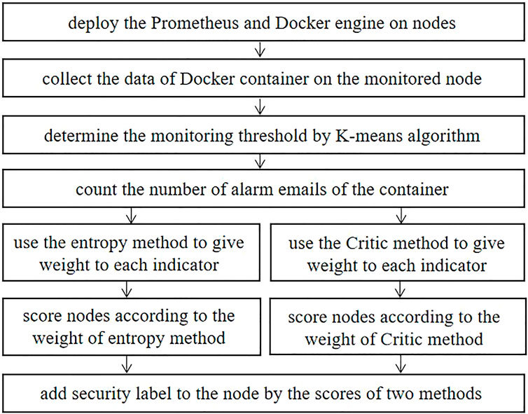
FIGURE 5. The security judgment scheme of the monitored node.

First, select the edge nodes as the monitoring node set $X_E$ and terminal nodes set $X_T$ under the edge computing network. The terminal node set $X_T$ includes n monitored nodes and m unmonitored nodes. The monitored node set is represented by $X_A$, the unmonitored node set is represented by $X_B$. The relationship among the three sets is $X_T=X_A\cup X_B$. The Docker container is deployed on the selected monitored node set $X_A$ as the security support engine, and the Prometheus monitoring software is deployed on the monitoring node set $X_E$ to collect the monitoring information of the container on the monitored node set $X_A$.

Second, collect the monitoring indicators of the monitored node set $X_A$. Each container collects k indicators. Assuming that there are i containers on each node, each node totally collects $i\times k$ indicators. In the monitored node set $X_A$, the monitoring indicators of the j-th node are shown as follows:

$\begin{array}{c}{A}_j^1={\left[j_1^1,j_2^1,\dots ,j_k^1\right]}^T\\ A_j^2={\left[j_1^2,j_2^2,\dots ,j_k^2\right]}^T\\ \begin{array}{c}:\\ A_j^i={\left[j_1^i,j_2^i,\dots ,j_k^i\right]}^T\end{array}\end{array}(15)$

where $j=\mathrm{1,2},\dots ,n$, $A_j^i$ represents the whole monitoring indicator of the i-th Docker container on the j-th node. $j_k^i$ in $A_j^i$ indicates k-th monitoring indicator of the i-th Docker container on the j-th node.

Third, according to the time ratio 1:1, setting the operation status of the container to normal operation and abnormal operation, respectively. Then, collect data of the j-th node in the monitored node set to get the sample set of container operation indicators $\mathrm{D}=\left(d_1,d_2,\dots ,d_n\right)$. Select a division $\mathrm{D}=D_1\cup D_2\cup \dots D_k$ so that $D_i\cap D_j=\varnothing ,\mathrm{i},\mathrm{j}\in \left[1,\mathrm{k}\right]$. After that, take $D_1$ as the testing set and $D_2,D_3,\dots ,D_k$ as the training set. Set the cluster result of parameter classification as 2, the maximum number of iterations as N, and selecting two data points in the sample set as the cluster center. K-means algorithm is used for dichotomous classification. Taking $D_1$ to $D_k$ as test sets, respectively, the lower bound of the risk indicator ${\sigma }_1,{\sigma }_2,\dots ,{\sigma }_k$ is obtained by clustering. The average value $\overline{\sigma }$ of ${\sigma }_1,{\sigma }_2,\dots ,{\sigma }_k$ is used as the monitoring threshold. The monitoring threshold value of each container follows

$\begin{array}{c}\overline{\sigma }\left(A_j^1\right)={\left[{\overline{\sigma }}_1^1,{\overline{\sigma }}_2^1,\dots ,{\overline{\sigma }}_k^1\right]}^T\\ \overline{\sigma }\left(A_j^2\right)={\left[{\overline{\sigma }}_1^2,{\overline{\sigma }}_2^2,\dots ,{\overline{\sigma }}_k^2\right]}^T\\ \begin{array}{c}:\\ \overline{\sigma }\left(A_j^i\right)={\left[{\overline{\sigma }}_1^i,{\overline{\sigma }}_2^i,\dots ,{\overline{\sigma }}_k^i\right]}^T\end{array}\end{array}(16)$

where $j=\mathrm{1,2},\dots ,n$, $\overline{\sigma }\left(A_j^i\right)$ represents monitoring indicator threshold of the i-th Docker container on the j-th node. ${\overline{\sigma }}_k^i$ indicates the k-th monitoring indicator threshold of the i-th Docker container.

Fourth, configure the alarm rules of Prometheus monitoring software. When any indicator of any container in the node exceeds the threshold, the Prometheus client on the edge monitoring node sends an alarm email to the specified mailbox. Count the number of indicator alarm messages received by all nodes in the specified mailbox within a certain time. ${\alpha }_{ij}$ represents the number of alarm messages received by the j-th indicator of the i-th node. The total number of alarm messages can be expressed in the following matrix:

$\alpha =\left[\begin{array}{ccc}{\alpha }_{11}& \cdots & {\alpha }_{1n}\\ ⋮& \ddots & ⋮\\ {\alpha }_{k1}& \cdots & {\alpha }_{kn}\end{array}\right](17)$

Fifth, the objective weighting method is used to give weight to each indicator. The objective weighting methods that we used include entropy weight method and Critic method. Score the node according to the weight, which will be computed by Eq. 18:

$S_i=100\times {\displaystyle \sum }_{j=1}^n{W}_j\times P_{ij}(18)$

where $W_j$ is the weight value of the j-th indicator, $P_{ij}$ is the ratio of the i-th sample to all samples of the j-th indicator. By setting the safety label division value, the score is divided into multiple segments, and the safety label information is added accordingly.

4 Security evaluation scheme of an unmonitored node

In edge computing networks, there may be some nodes that do not install the Docker engine and monitoring model. In this section, we provide a novel scheme based on the ideas of community detection and PageRank algorithm to evaluate the security of unmonitored nodes, which will predict the security state of the unmonitored nodes by taking advantages of the Docker nodes. The basic theory including the community detecting and the PageRank algorithm will be introduced in Section 4.1. Section 4.2 will illustrate the specific steps of the novel method.

4.1 Theory

4.1.1 Community detection

The community detecting algorithm is a segmentation algorithm that is based on the graph model (Yang and Cao, 2022). Its basic purpose is to divide the nodes in the graph model into several communities, so that there is a closer connection between the nodes in the community (Hu et al., 2020). In this paper, the community detecting algorithm is used to segment the graph model and determine the security label of each node. We chose four classical algorithms—LPA, SLPA, Louvain, and GN—to divide the community and we then compared their division result through modularity.

LPA and SLPA algorithms are community detecting algorithms that are based on the label propagation (Li et al., 2015). The basic principle of LPA is that according to the connection relationship between nodes in the graph model, the labels of each node are diffused to the whole graph to obtain stable results, and the nodes with the same label are divided into the same community (Ravi Kiran, 2011). Compared with LPA, SLPA is different in that it introduces the strategies of the listener and speaker. The speaker node sends label information to each listener node connected to the speaker node according to a certain propagation method (Gupta, 2022). The listener node that receives the label selects the transferring label of each speaker node according to a certain receiving method.

In contrast from the label propagation idea of the LPA and SLPA algorithm, the Louvain algorithm is designed based on modularity $\mathrm{Q}$. It regards each node as a community, and merges each node and its adjacent nodes into a new community. It then iterates until modularity is stable. Modularity is the evaluation index used to measure the advantages and disadvantages of community division. It is the first evaluation index to measure the quality of community division results (Su and Havens, 2015). This index is mainly used to measure the results of community division in the undirected graph without weight. The calculation method of modularity $\mathrm{Q}$ is given as follows:

Suppose that the graph model is divided into k communities, then define a $k\times k$ Matrix $\mathrm{e}$, and the element $e_{ij}$ in the matrix represents the proportion of the number of edges connecting the i-th community and the j-th community in the total number of edges. The trace of matrix e represents the set of edges between nodes in the same community, which is calculated by

$Tre={\displaystyle \sum }_i{e}_{ii}.(19)$

The trace of the matrix alone cannot fully reflect the community structure because when the graph model is divided into only one community, the trace of the matrix is 1. Therefore, a new value $a_i$ is defined to represent the proportion of the number of edges connected to the i-th community in the total number of edges. The computing method of $a_i$ follows:

$a_i={\displaystyle \sum }_j{e}_{ij}.(20)$

According to the above two definitions, the computing method of modularity $\mathrm{Q}$ is given as:

$Q={\displaystyle \sum }_i\left(e_{ii}-a_i^2\right).(21)$

The GN algorithm is a community that is based on discovery method based on modularity and betweenness of the edge. Assume that the community division of the graph has been obtained. We can regard that there are fewer edges between communities and more edges within communities. The idea of the GN algorithm is to remove edges between communities (Shukla, 2022b). The concept of edge-betweenness is proposed to describe the “importance” of edges. The betweenness of the edge is defined as the number of the shortest paths through this edge in the graph. The GN algorithm removes the edge with the largest edge-betweenness in each iteration until the modularity reaches a local peak value.

The workflow of the GN algorithm is shown in Figure 6. First, input the graph structure and the number of nodes. We then set the initial modularity $Q_0$. Then, count the betweenness of each edge in the graph. Afterward, remove the edge with the largest betweenness to form a new graph. For the new graph, compute the modularity $Q_i$ after i-th iteration. The next step is to minimize the modularity of the graph. The GN algorithm compares the modularity $Q_i$ of the new graph with the initial modularity $Q_0$. After that, judge whether the modularity $Q_i$ of the new graph is locally optimal. If $Q_i\le Q_0$, then terminate the algorithm and output the community division result. If $Q_i>Q_0$, then set $Q_0=Q_i$ and turning back to step 2. Compute the betweenness and removing the edge with the largest betweenness to update the graph by the iteration. Terminate the algorithm until the modularity $Q_i$ reaches the local optimization. It must be noted that the termination condition of the algorithm is not necessary to make the modularity $Q_i$ locally optimal. Although we introduced one of the termination conditions, the termination of the algorithm changes according to the actual situation.

FIGURE 6

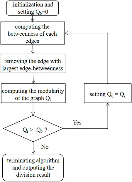
FIGURE 6. The workflow of the GN algorithm.

4.1.2 PageRank algorithm

The PageRank algorithm is an algorithm for Google Web page recommendation, which was first proposed by Google founder Larry Page. Based on the idea of the random walk, the algorithm evaluates the relevance and importance of web pages according to the user’s access records (Sharma et al., 2022a). By using the connectivity between web pages to judge the importance of web pages, the correlation is quantified as a PR value and an optimal solution is obtained through continuous iteration (Hao, 2015). The specific steps of the algorithm are described as follows:

Step 1. First, initialize the same PR value for each node. Generally, the access probability is used as the PR value of the node; that is, the initial PR value of each node is $\raisebox{1ex}{$1$}\!\left/ \!\raisebox{-1ex}{$N$}\right.$, and N is the number of all nodes in the community. To make the PR value of the two iterations fully close and the output of the algorithm tend to be stable, we set the parameter ${ϵ}_0$. When the error of two iterations is smaller than ${ϵ}_0$, the algorithm is terminated.

Step 2. Suppose that the user starts from a node and randomly selects a node connected to the current node as the next access node. Each node distributes the currently accessed PR value to all nodes that the node may access, and updates its own PR value through the PR value transmitted by other nodes. The update method is shown as follows:

$\mathit{PR}\left(x\right)=\frac{1-\alpha }{N}+\alpha {\displaystyle \sum }_{i=1}^n\frac{\mathit{PR}\left(T_i\right)}{C\left(T_i\right)},(22)$

where $N$ is the total number of all nodes, node $T_i$ belongs to one of all nodes to which node $x$ is connected, and $C\left(T_i\right)$ represents the number of all nodes to which node $T_i$ can connect, $\alpha$ is the damping coefficient.

Step 3. Repeat Step 2 until the error satisfies the condition $ϵ<{ϵ}_0$. Obtain the possible access probability of each node and output the results.

$ϵ=\left|P_{n+1}-P_n\right|.(23)$

4.2 Scheme for node security evaluation without monitoring

In this subsection, we propose a new security evaluation scheme for unmonitored terminal nodes in the edge computing scenario. In an edge computing network, not all nodes can use Docker as a security engine. Some nodes with Docker container can judge the security through monitoring model, while others are not monitored. Therefore, a new scheme based on the graph to evaluate the security of unmonitored nodes through the security of monitored nodes is proposed. The novel method will be illustrated in detail, and the specific steps are shown in Figure 7.

FIGURE 7

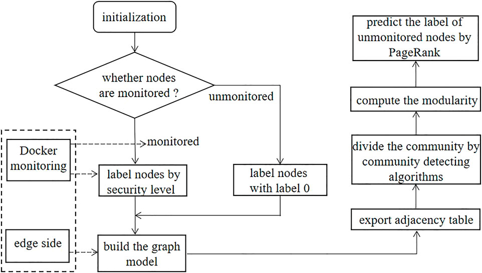
FIGURE 7. The workflow of security evaluation method of the unmonitored node.

According to the proposed security judgment method of the monitored node described in Section 3, we collect the monitoring indicators of each container on the node and label the node with security label. If the node is monitored by container technology, then we can label the node by its security level. Otherwise, the unmonitored node is labeled with label 0. Based on the connection relationship of each node, the Neo4j software is used to establish the graph model and generate the adjacency matrix and adjacency table.

The adjacency table is used as the input data set of the community detecting algorithm. Four algorithms are used to divide the community. We calculate and compare the average of the community partition results of each algorithm. The modularity of the Louvain algorithm is represented by $Q_{Lv}$ and the modularity of the GN algorithm is represented by $Q_{GN}$. The LPA and the SLPA algorithm will lead to multiple results. We use the statistics the probability of each classification result and weighted average the modularity of each result. $P_L^i$ and $P_S^i$ represent the probability of each result of the LPA and SLPA, respectively. The modularity of each division of each of the results of the LPA and SLPA are indicated by $Q_L^i$ and $Q_S^i$, respectively. The computing method of the total modularity of the LPA algorithm and SLPA algorithm follows:

$\overline{Q_L}={\displaystyle \sum }_{i=1}^a{P}_L^i\times Q_L^i(24)$

$\overline{Q_S}={\displaystyle \sum }_{i=1}^b{P}_S^i\times Q_S^i(25)$

The purpose of community division is to divide nodes with stronger relevance into the same community. We compared the community partition results of four algorithms by modularity. After the algorithm results with better classification are obtained, we chose the unmonitored node as the initial node and used the PageRank algorithm to predict the access probability of initial node to the other monitored nodes. If the initial node has higher probability to access the node with high-risk label, then it is evaluated to be higher risk. If it has higher probability to access the node with low-risk label, then it is predicted to be lower risk. The probability of accessing high-risk label nodes is represented by $P_h$, the probability of accessing medium-risk label nodes is $P_m$, and the probability of accessing low-risk label nodes is represented by $P_l$.

5 Experimental results

We set up the experiment under the power system to verify the effectiveness and feasibility of the proposed novel scheme. In the power system, the container monitoring model were deployed in two different real scenarios, including smart energy system and relay protection system. The Docker technology was used as the security engine in the different systems. All of the applications in the server were encapsulated in the Docker container. They were run in isolation from each other to ensure their own safety. The power edge board can be used to collect and process meter data, and has certain computing power. We installed the Docker engine on it. We used three Windows desktop computers as the monitoring node set $X_E=\left\{A_{13},A_{14},A_{15}\right\}$, and 12 power edge boards are used to simulate terminal node set $X_T$, which includes nine monitored nodes and three unmonitored nodes. Nine monitored nodes to form a set of monitored nodes $X_A=\left\{A_1,A_2,A_3\dots A_9\right\}$. Three unmonitored nodes constitute a set of unmonitored nodes $X_B=\left\{A_{10},A_{11},A_{12}\right\}$. The Docker engine and Cadvisor software were installed on the set of monitored nodes $X_A$. Each node deploys 1 Docker container. The Prometheus server collects the Docker container running data from the container on monitored nodes. In addition, we construct a private Docker registry to ensure the security of the Docker image. The specific steps of the configuration follow:

The configuration of the Docker environment consists of two parts: the installation of Docker engine on the host and the establishment of the Docker private image registry. Docker technology can be regarded as a lightweight virtual machine technology, which is also implemented through the Linux container function. The prerequisite for installing Docker on the Windows system is that the system must support Hyper-V virtualization. Docker officially released the Docker for desktop version under the Windows system (the installation can be directly downloaded from the Docker official website https://www.Docker.com). After successful installation, add the Docker installation directory to the path environment variable, restart the computer, and click the desktop Docker icon to run Docker.

The Docker private image registry needs to be established in the monitoring model. We will next describe how to establish a private Docker image registry and upload the compiled image. Users can use the browser to access http://localhost:5000/v2/_catalog to view the new image uploaded to the private Docker image registry. The specific steps are as follows:

Enter the Docker command “Docker pull registry” in the command line to download the registry image from Dockerhub;

Enter “Docker run—it registry bin/bash,” create containers by registry images, and build private Docker image registry;

Create a new container using the existing Docker image;

Compile the Docker private image, enter the command “Docker commit container ID + image name” to compile the Docker container into a new image;

Enter “Docker tag + image name + 127.0.0.1:5000/+ image name” to label the new image;

Enter “Docker pull + 127.0.0.1:5000/+ image name” to upload the Docker image to the private Docker image registry.

The Prometheus software of the edge node is configured with Docker container monitoring indicators. In this experiment, a total of five container monitoring indicators are selected (i.e., CPU occupancy, memory occupancy, input flow, output flow and block read flow). When one or more indicators exceed the threshold, Prometheus software sends an alarm email to the specified mailbox. Prometheus is connected with Grafana in the form of HTTP to visually display the monitoring indicators. The specific operation is as follows:

First, enter the Docker command “Docker pull Google/cadvisor” to pull the Docker image of the Cadvisor from the Docker official image registry. Next, create a new container by this image to run the Cadvisor component. Users can login to the http://localhost:8080/ port to view the monitoring indicators collected by Cadvisor.

Install the Prometheus software on the monitoring node set $X_E$. The Cadvisor component exposes the monitoring indicators to Prometheus monitoring software through HTTP connection, and configures container monitoring and alarm rules. Additionally, the alarm module is realized through the Alertmanager component under Prometheus and the alarm rule is set to use email alarm. Users can configure the YML file to set receiving mailbox and alarm mail type. The Grafana component finally is used to achieve the visual display. The user enters the Docker command “Docker pull grafana/grafana” to download the Grafana image and create a Docker container by this image. The visual interface can be viewed by logging into the website at http://localhost:3000.

Each monitored node includes five monitoring indicators, the monitoring indicators of the container on the j-th node are expressed as $A_j^1={\left[j_1^1,j_2^1,j_3^1,j_4^1,j_5^1\right]}^T,j\in \left[\mathrm{1,9}\right]$. The Prometheus server collects five Docker container running indicators from the container on the monitored node every second. We set the container to normal state and abnormal state respectively, and make them run for 5 min in both states to collect a total of 600 pieces of data. Repeat the operation for 10 times to get 10 monitoring data sets. Afterward, the K-means algorithm is used to divide the data into two categories by setting $\mathrm{K}=2$. We take the average value of the lower bound of abnormal data in 10 classifications $\overline{\sigma }={\left[{\overline{\sigma }}_1^1,{\overline{\sigma }}_2^1,{\overline{\sigma }}_3^1,{\overline{\sigma }}_4^1,{\overline{\sigma }}_5^1\right]}^T$ as the monitoring threshold, where ${\overline{\sigma }}_1^1$ represents the first monitoring indicator of the first container, ${\overline{\sigma }}_2^1$ represents the second monitoring indicator of the first container and so on. The Docker container monitoring indicator threshold is shown in Table 1. Configure the Prometheus alarm rules of the edge node according to the monitoring threshold $\overline{\sigma }$. When the monitoring value is bigger than the operation indicator threshold, the Prometheus client sends an alarm email to the specified mailbox.

TABLE 1

TABLE 1. Docker container monitoring indicator threshold.

5.1 Security results of a monitored node

After deploying the monitoring model, we proposed a novel scheme to judge the security of monitored nodes in the terminal node set $X_T$. In this experiment, the terminal node is achieved by the power edge board. By counting the number of alarm emails received by nine monitored nodes within 24 h, we get a $9\times 5$ matrix $\alpha$, where ${\alpha }_{ij}$ indicates the number of alarm messages received by the i-th indicator of the j-th node. From left-hand to right-hand, each row of the matrix indicates CPU alarm times, memory alarm times, input network traffic alarm times, output network traffic alarm times and block read traffic alarm times. The entropy weight method and the Critic method are used to weigh and score each monitoring indicator. The scoring value is divided into three segments, based on which three security levels of nodes are given, and the label collection of nine monitored nodes is obtained.

Configuring the monitoring rule according to monitoring threshold, and the result matrix $\alpha$ is obtained by counting the number of Prometheus sends alarm emails, as shown below. ${\alpha }_{ij}$ represents the j-th monitoring indicator of the i-th node.

$\alpha =\left[\begin{array}{ccccc}3& 0& 1& 1& 0\\ 0& 1& 1& 2& 0\\ 1& 1& 0& 0& 1\\ 1& 1& 3& 0& 0\\ 1& 0& 4& 0& 0\\ 0& 1& 0& 1& 2\\ 0& 1& 0& 0& 1\\ 0& 0& 0& 0& 1\\ 1& 0& 0& 2& 0\end{array}\right](26)$

Before weighting the indicator, the matrix $\alpha$ carries out standardization processing to obtain the data standardization matrix β, which is shown as

$\beta =\left[\begin{array}{ccccc}0.9960& 0.0020& 0.2505& 0.4990& 0.0020\\ 0.0020& 0.9960& 0.2505& 0.9960& 0.0020\\ 0.3333& 0.9960& 0.0020& 0.0020& 0.4990\\ 0.3333& 0.9960& 0.7475& 0.0020& 0.0020\\ 0.3333& 0.0020& 0.9960& 0.0020& 0.0020\\ 0.0020& 0.9960& 0.0020& 0.4990& 0.9960\\ 0.0020& 0.9960& 0.0020& 0.0020& 0.4990\\ 0.0020& 0.0020& 0.0020& 0.0020& 0.4990\\ 0.3333& 0.0020& 0.0020& 0.0020& 0.0020\end{array}\right](27)$

The entropy method and the Critic method are used to weigh the result matrix $\alpha$ and the weight of each indicator is computed, as shown in Table 2. The classification principle follows the principle that the higher the weighted value, the higher the risk of nodes. In the weighting results of the entropy method, the weight of output flow and input flow is the largest. This indicates that the information entropy of these two indicators is smaller and the degree of information variation is the highest, which is more important in the overall evaluation system. The weight value of the memory indicator is the smallest. This indicates that the indicator has greater information entropy and a low degree of information variation, which is the least important in the overall evaluation system. Among the weighting results of the Critic method, the weight of memory occupancy rate is the largest. This indicates that the correlation between indicator memory occupancy rate and other indicators is lower. The weight of CPU occupancy is the smallest. This indicates that the correlation between CPU occupancy and other indicators is higher. The two weighting methods are basically consistent in the weighting of indicator CPU occupancy and indicator block device reading. In terms of indicator memory occupancy, the weight given by the entropy method is far less than that given by the Critic method. In terms of input and output flow, the weight given by the entropy method is slightly higher than that given by the Critic method.

TABLE 2

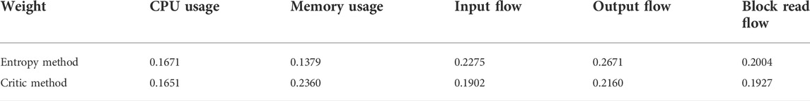
TABLE 2. Weight of the objective weighting method.

The scoring results of each monitored node in $X_A$ are shown in Figure 8. Using the same threshold division and comparing the scoring results of the entropy weight method and the Critic method, it can be regarded that the results are basically the same. The scoring results of node $A_8$ and node $A_9$ are small, which means they are in a low-risk state. The scoring results of nodes $A_1$, $A_2$ and $A_6$ are in a high-risk state. Intermediate node $A_3$, node $A_4$ and node $A_5$ can be determined to be in a medium-risk state. Only node $A_7$ is in an unstable state under the current threshold and the score result of the entropy method is lower, so it is judged to be in a low-risk state. The score of Critic method is slightly higher, and it is judged as medium-risk. We take a division interval [0,9], [9,14], [14,20] to make the two methods have the same security division result. When score $S_i\in \left[0,9\right]$, it is determined that the node is in a low-risk state and label 1 is assigned to the node. When score $S_i\in (9,14]$, it is determined that the node is in a medium-risk state and label 2 is assigned to the node. When score $S_i\in (14,20]$, it is determined that the node is in a high-risk state. It can be determined that node 1, node 2 and node 6 are in a high-risk state. Node $A_3$, node $A_4$, node $A_5$ and node $A_8$ are in the medium-risk state, and node $A_7$ and node $A_9$ are in the low-risk state. We can add labels to the nodes according to the scoring result of two methods to form key value pairs [$A_1,3$], [$A_2,3$], [$A_3,2$], [$A_4,2$], [$A_5,2$], [$A_6,3$], [$A_7,2$], [$A_8,1$], [$A_9,1$].

FIGURE 8

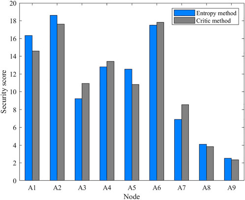
FIGURE 8. Security score of the Entropy method and the Critic method.

5.2 Security results of an unmonitored node

After labeling the node by the security judgment method, the graph model is established according to the connection relationship of each node under the edge side network, as shown in Figure 9. The nodes in the terminal node set $X_T=\left\{A_1,A_2,\dots ,A_{12}\right\}$ are represented by the solid line circles. The blue circles represent monitoring nodes, red circles represent high-risk nodes, the yellow circles represent medium-risk nodes, the green circles represent low-risk nodes, and unmonitored nodes are represented by dotted line circles. The nodes in edge node set $X_E=\left\{A_{13},A_{14},A_{15}\right\}$ because monitoring nodes are in low-risk state by default. The graph model is derived as an adjacency table as follows: [4 14, 1 12, 3 15, 8 15, 3 9, 9 15, 11 14, 13 14, 12 15, 14 15, 13 15, 5 14, 7 11, 7 13, 1 13, 10 13, 2 13, 5 6, 6 14].

FIGURE 9

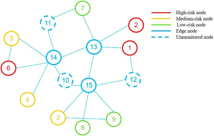
FIGURE 9. The graph model built on edge side.

The LPA and the SLPA will lead to multiple division results. We count the probability of each result and compute the modularity by weighted average method. Taking the adjacency table as the input, the LPA is used to divide the community of the model, and the algorithm is run repeatedly for 10 times to obtain three division results. The first division result is [4,5,6,14], [3,8,9,15], [1,2,7,10,11,12,13]. The second division result is [3,8,9,15], [4,5,6,11,14], [1,2,7,10,12,13]. The third division result is [3,8,9,12,15], [1,2,10,13], [4,5,6,7,11,14].

To compare the classification results of the algorithms, the concept of modularity is introduced to measure. Compute the modularity of each classification result to get the modularity of three division result $Q_L^1=0.3920$, $Q_L^2=$ 0.4003 $Q_L^3=0.3947$. The probability of result 1 in 10 experiments is 0.2, the probability of result 2 is 0.65, and the probability of result 3 is 0.15. According to the probability of the three results, the total modularity of LPA is obtained after weighted computing of each modularity $\overline{Q_L}=0.3978$.

The SLPA is used to divide the community of the model. Repeat the operation for 10 times and remove the division results of overlapping communities and missing nodes. We obtain two kinds of division results of communities without loss and repeated division. The first division is [1, 12], [2, 4, 5, 6, 7, 10, 11, 13, 14], [3, 8, 9, 15]. The second division is [1, 2, 7, 10, 12, 13], [4, 5, 6, 11, 14], [3, 8, 9, 15]. Compute the modularity of each classification result to get the modularity of the first division result $Q_S^1=0.3283$ and the modularity of the second division result $Q_S^2=0.7050$. The probability of result 1 in 10 experiments is 0.78 and the probability of result 2 is 0.22. The total modularity of SLPA is obtained after weighted computing of each modularity $\overline{Q_S}=$ 0.4112.

When compared to the LPA and SLPA algorithms, the Louvain and the GN algorithms are more stable. For these two algorithms, only one division result will be generated separately. The division of the Louvain algorithm is [11, 7], [4, 5, 6, 14], [3, 8, 9, 10, 15], [2, 1, 12, 13]. Similarly, computing the modularity of the division to get $Q_{Lv}=0.5789$. The result of the GN algorithm is shown in Figure 10. The division is [4, 5, 6, 10, 14], [1, 2, 12, 13], [3, 8, 9, 15], [11, 7]. Computing the modularity of the division to get $Q_{GN}=0.8144$.

FIGURE 10

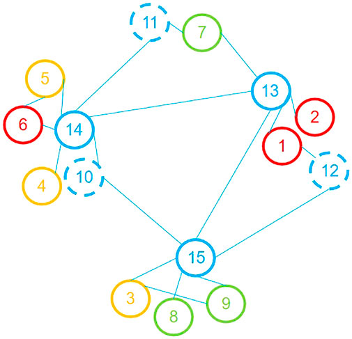
FIGURE 10. The division result of the GN algorithm.

We used four community detection algorithms to divide the community for this graph model. The comparison of the four algorithms is shown in Table 3. The letter m represents the number of edges in the graph and the letter n represents the number of nodes in the graph.

TABLE 3

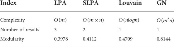
TABLE 3. The comparison of four community detection algorithms.

In Table 3, we can see the division results of the LPA and the SLPA are unstable and their community division results are random. Comparing the modularity of the four algorithms, it is easy to find that $Q_{GN}>Q_{Lv}>\overline{Q_S}>\overline{Q_L}$. Although the complexity of the GN algorithm is larger than the other three algorithms, because the graph model established in this article is not complex, the slightly lower efficiency of GN algorithm is acceptable. Therefore, we select the community division result of the GN algorithm. There are four communities—[4, 5, 6, 10, 14], [1, 2, 12, 13], [3, 8, 9, 15], and [11, 7]—in the division result.

Nodes in the same community have stronger correlation. We assume that a user randomly accesses any associated node in the community from an unmonitored node. The access probability of each node is described by the PR value. We evaluate the security of the initial node by its access probability to each node. If the user has a higher probability of accessing high-risk nodes, then we evaluate that the initial node (unmonitored node) has a higher correlation with the high-risk node, and the risk of the node is also higher. In contrast, if the user has a higher probability of accessing low-risk nodes, then we evaluate that the risk of the initial node is lower. Setting the error ${ϵ}_0=0.0001$ to make sure the PR value of the two iterations fully close and the algorithm tends to be stable. The number of the node in community is $\mathrm{N}=5$_,and the initial PR value of each node $\mathit{PR}\left(x\right)=\raisebox{1ex}{$1$}\!\left/ \!\raisebox{-1ex}{$N$}\right.=0.2$. This means that the unmonitored nodes have equal probability to access the whole nodes in the initial state. In community [4, 5, 6, 10, 14], we take $A_{10}$ as the initial node and use PageRank algorithm to update the PR value until $\left|P_{n+1}-P_n\right|<ϵ$. The PR value is shown in Table 4.

TABLE 4

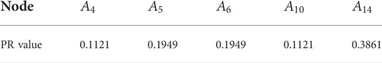
TABLE 4. The PR value when ${\mathit{A}}_{10}$ is taken as the initial node.

In Table 4, Node $A_{14}$ is low-risk node, nodes $A_4$ and $A_5$ are medium-risk nodes, node $A_6$ is high-risk node, and nodes $A_{10}$ is unmonitored node. We can calculate that the probability that node $A_{10}$ may access the high-risk label in probability of $P_h=0.1949$, the probability of accessing the medium-risk label is $P_m=0.3070$, and the probability of accessing the low-risk label is $P_l=0.3861$. It can be evaluated that node $A_{10}$ is a low-risk node.

Similarly, we take $A_{12}$ as the initial node and use the PageRank algorithm to update the PR value in community [1, 2, 12, 13], the PR value is shown in Table 5. Node $A_1$ and $A_2$ are in high-risk state, node $A_{13}$ is a low-risk node, and node $A_{12}$ is an unmonitored node. We can count that $A_{12}$ has the probability of $P_h=0.5000$ to access the high-risk node. The probability of accessing the low-risk node is $P_l=0.3246$. Therefore, node $A_{12}$ is judged as a high-risk node. Because node $A_{11}$ is only in the same community with a high-risk node $A_7$, it is judged that node $A_{12}$ is in the low-risk state.

TABLE 5

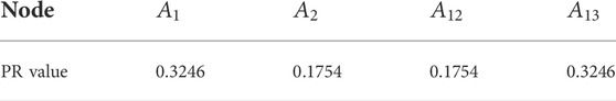
TABLE 5. The PR value when ${\mathit{A}}_{12}$ is taken as the initial node.

We combined the community detecting algorithms and the PageRank algorithm to provide a method to preliminarily evaluate the security of unmonitored nodes, but this method still has defects. On the one hand, the community division algorithm is used to divide the more closely connected nodes into the same community. When we chose the community detecting algorithm, we were concerned about the stability of algorithms and compared their division results by the modularity. However, the complexity of the algorithm should also be concerned in the actual scenario. A larger algorithm complexity means more computing resource consumption. In our experiment, the GN algorithm has the largest modularity but the highest complexity. The graph model that is built in our paper is simple (15 nodes and 19 edges). In the real scene, the graph model usually is constructed by millions of nodes and edges. Therefore, it is necessary to consider the algorithm complexity and computing resource consumption in real scenarios. On the other hand, the PageRank algorithm assumes that the user walks randomly within the community and indirectly evaluates the security of nodes according to the probability of users accessing each label. In this method, the label of the unmonitored nodes highly depends on the label in the same community. Taking the division result of the GN algorithm as an example, node $A_7$ and node $A_{11}$ belong to the same community, and there are no other nodes in the community, the label value of the unmonitored node $A_{11}$ completely depends on node $A_7$. Therefore, the premise of using this method is that there should be more nodes with known labels in the community than unmonitored nodes.

6 Conclusion

This paper developed a security scheme using a Docker container in the edge computing system. A container risk monitoring model based on container monitoring software was designed. Based on Docker monitoring, we proposed a novel node security judgment scheme under Docker monitoring. Meanwhile, a new security evaluation scheme for unmonitored nodes through the node security judgment scheme was proposed. Finally, we built a container monitoring model for a power system and verified the feasibility of the proposed method by experiment, which proved that our scheme is highly secure to the EC protection.

Data availability statement

The original contributions presented in the study are included in the article/supplementary material, and further inquiries can be directed to the corresponding author.

Author contributions

XX: conceptualization, methodology, software, writing—original draft; YJ: resource, formal analysis; HW: writing—review and editing, supervision, project administration; WH: writing—review and editing; SC: data curation, visualization.

Conflict of interest

Author YJ was employed by China Southern Power Grid Co Ltd.

The remaining authors declare that the research was conducted in the absence of any commercial or financial relationships that could be construed as a potential conflict of interest.

Publisher’s note

All claims expressed in this article are solely those of the authors and do not necessarily represent those of their affiliated organizations, or those of the publisher, the editors and the reviewers. Any product that may be evaluated in this article, or claim that may be made by its manufacturer, is not guaranteed or endorsed by the publisher.

References

Abhishek, M. K., and Rajeswara Rao, D. (2021). Framework to secure docker containers,” in 2021 Fifth World Conference on Smart Trends in Systems Security and Sustainability. London, United Kingdom: WorldS4, 152–156.

CrossRef Full Text | Google Scholar

Agarwal, S. (2022). “GUI docker implementation: Run common graphics user applications inside docker container,” in 2021 10th International Conference on System Modeling & Advancement in Research Trends (SMART) MORADABAD, India, 424

Google Scholar

AII (2018). Introduction to edge computing in IIoT. Available at: https://www.iiconsortium.org/pdf/Introduction_to_Edge_Computing_in_IIoT_2018-06-18-updated.pdf (Accessed on June 18, 2018).

Google Scholar

Cai, L., Qi, Y., Wei, W., and Li, J. (2019). Improving resource usages of containers through auto-tuning container resource parameters. IEEE Access 7, 108530–108541. doi:10.1109/ACCESS.2019.2927279

CrossRef Full Text | Google Scholar

Chatterjee, I. (2021). Artificial intelligence and patentability: Review and discussions. Int. J. Mod. Res. 1, 15–21. doi:10.1093/oso/9780198870944.003.0006

CrossRef Full Text | Google Scholar

ECC and AII (2019). The edge computing advantages. Available at: https://www.iiconsortium.org/pdf/IIC_Edge_Computing_Advantages_White_Paper_2019-10-24.pdf (Accessed on Octorber 24, 2019).

Google Scholar

ECC (2016). White paper of edge computing consortium. Available at: http://www.ecconsortium.net/Uploads/file/20161208/1481181867831374.pdf (Accessed on November 28, 2016).

Google Scholar

Esteves, R. M., et al. (2013). Competitive K-means, a new accurate and distributed K-means algorithm for large datasets in 2013 IEEE 5th International Conference on Cloud Computing Technology and Science (Bristol, UK), 17–24.

CrossRef Full Text | Google Scholar

Gupta, V. K. (2022). Crime tracking system and people’s safety in India using machine learning approaches. Int. J. Mod. Res. 2 (1), 1–7. doi:10.1109/indiscon53343.2021.9582222

CrossRef Full Text | Google Scholar

Hao, Z. (2015). “An improved PageRank algorithm based on web content,” in 2015 14th International Symposium on Distributed Computing and Applications for Business Engineering and Science (Guiyang, China): DCABES), 284.

CrossRef Full Text | Google Scholar

Hu, J., Du, Y., and Liu, J. (2020). Detecting and evolving microblog community based on structure and gravity cohesion. IEEE Access 8, 176624–176639. doi:10.1109/ACCESS.2020.3022836

CrossRef Full Text | Google Scholar

Jiang, W., Wang, Y., Huang, Y., and Zhao, Q. (2019). Top invulnerability nodes mining in dual-direction different-weight complex network based on node double-level local structure weighted entropy. IEEE Access 7, 86597–86610. doi:10.1109/ACCESS.2019.2925572

CrossRef Full Text | Google Scholar

Khorramabadi, S. S., and Bakhshai, A. (2015). Intelligent control of grid-connected microgrids: An adaptive critic-based approach. IEEE J. Emerg. Sel. Top. Power Electron. 3, 493–504. doi:10.1109/JESTPE.2014.2331188

CrossRef Full Text | Google Scholar

Kumar Pentyala, S. (2017). “Emergency communication system with Docker containers, OSM and Rsync,” in 2017 International Conference On Smart Technologies For Smart Nation (SmartTechCon) (Bengaluru, India), 1064–1069.

CrossRef Full Text | Google Scholar

Kumar, R., and Dhiman, G. (2021). A comparative study of fuzzy optimization through fuzzy number. Int. J. Mod. Res. 1, 1–14. doi:10.1109/icmlc.2007.4370325

CrossRef Full Text | Google Scholar

Kushida, T., and Pingali, G. S. (2014). Industry cloud - effective adoption of cloud computing for industry solutions,” in IEEE 7th International Conference on Cloud Computing. Anchorage, AK, USA), 753–760.

CrossRef Full Text | Google Scholar

Kwon, S., and Lee, J. -H. (2020). Divds: Docker image vulnerability diagnostic system. IEEE Access 8, 42666–42673. doi:10.1109/ACCESS.2020.2976874

CrossRef Full Text | Google Scholar

Li, H., Lu, H., Lin, Z., Shen, X., and Price, B. (2015). Inner and inter label propagation: Salient object detection in the wild. IEEE Trans. Image Process. 24, 3176–3186. doi:10.1109/TIP.2015.2440174

PubMed Abstract | CrossRef Full Text | Google Scholar

Liu, Q., Zheng, W., Zhang, M., Wang, Y., and Yu, K. (2018). Docker-based automatic deployment for nuclear fusion experimental data archive cluster. IEEE Trans. Plasma Sci. IEEE Nucl. Plasma Sci. Soc. 46, 1281–1284. doi:10.1109/TPS.2018.2795030

CrossRef Full Text | Google Scholar

Liu, Y., Shou, G., Chen, Y., and Chen, S. (2020). Toward edge intelligence: Multiaccess edge computing for 5G and Internet of things. IEEE Internet Things J. 7, 6722–6747. doi:10.1109/JIOT.2020.3004500

CrossRef Full Text | Google Scholar

Muñoz, R., Vilalta, R., Yoshikane, N., Casellas, R., Martinez, R., Tsuritani, T., et al. (2018). Integration of IoT, transport SDN, and edge/cloud computing for dynamic distribution of IoT analytics and efficient use of network resources. J. Light. Technol. 36, 1420–1428. doi:10.1109/JLT.2018.2800660

CrossRef Full Text | Google Scholar

Neshenko, N., Bou-Harb, E., Crichigno, J., Kaddoum, G., and Ghani, N. (2019). Demystifying IoT security: An exhaustive survey on IoT vulnerabilities and a first empirical look on internet-scale IoT exploitations. IEEE Commun. Surv. Tutorials 21, 2702–2733. doi:10.1109/COMST.2019.2910750

CrossRef Full Text | Google Scholar

Rabay'a, A. (2019). “Fog computing with P2P: Enhancing fog computing bandwidth for IoT scenarios,” in 2019 International Conference on Internet of Things (iThings) (Atlanta, GA, USA), 82–89.

Google Scholar

Rahmansyah, R., et al. (2021). “Reducing docker daemon attack surface using rootless mode,” in 2021 International Conference on Software Engineering & Computer Systems and 4th International Conference on Computational Science and Information Management (ICSECS-ICOCSIM) (Pekan, Malaysia: ICSECS-ICOCSIM), 499

CrossRef Full Text | Google Scholar

Ravi Kiran, B. (2011). “An improved connected component labeling by recursive label propagation,” in 2011 National Conference on Communications (NCC) (Bangalore, India), 1

CrossRef Full Text | Google Scholar

Reis, D., Piedade, B., Correia, F. F., Dias, J. P., and Aguiar, A. (2022). Developing docker and docker-compose specifications: A developers’ survey. IEEE Access 10, 2318–2329. doi:10.1109/ACCESS.2021.3137671

CrossRef Full Text | Google Scholar

Şengül, Ö. (2021). “Implementing a method for docker image security,” in 2021 International Conference on Information Security and Cryptology (ISCTURKEY) (Ankara, Turkey: ISCTURKEY), 34.

Google Scholar

Sharma, T. (2022a). Breast cancer image classification using transfer learning and convolutional neural network. Int. J. Mod. Res. 2 (1), 8–16. doi:10.31234/osf.io/w9rb2

CrossRef Full Text | Google Scholar

Shukla, S. K. (2022b). Self-aware execution environment model (SAE2) for the performance improvement of multicore systems. Int. J. Mod. Res. 2 (1), 17–27. doi:10.1002/cpe.2948

CrossRef Full Text | Google Scholar

Smet, P., Dhoedt, B., and Simoens, P. (2018). Docker layer placement for on-demand provisioning of services on edge clouds. IEEE Trans. Netw. Serv. Manage. 15, 1161–1174. doi:10.1109/TNSM.2018.2844187

CrossRef Full Text | Google Scholar

Song, C., Han, G., and Zeng, P. (2022). Cloud computing based demand response management using deep reinforcement learning. IEEE Trans. Cloud Comput. 10, 72–81. doi:10.1109/TCC.2021.3117604

CrossRef Full Text | Google Scholar

Song, C., Sun, Y., Han, G., and Rodrigues, J. J. (2021a). Intrusion detection based on hybrid classifiers for smart grid. Comput. Electr. Eng. 93, 107212–107310. doi:10.1016/j.compeleceng.2021.107212

CrossRef Full Text | Google Scholar

Song, C., Xu, W., Han, G., Zeng, P., Wang, Z., and Yu, S. (2021b). A cloud edge collaborative intelligence method of insulator string defect detection for power IIoT. IEEE Internet Things J. 8, 7510–7520. doi:10.1109/JIOT.2020.3039226

CrossRef Full Text | Google Scholar

Su, J., and Havens, T. C. (2015). Quadratic program-based modularity maximization for fuzzy community detection in social networks. IEEE Trans. Fuzzy Syst. 23, 1356–1371. doi:10.1109/TFUZZ.2014.2360723

CrossRef Full Text | Google Scholar

Taleb, T., Samdanis, K., Mada, B., Flinck, H., Dutta, S., and Sabella, D. (2017). On multi-access edge computing: A survey of the emerging 5G network edge cloud architecture and orchestration. IEEE Commun. Surv. Tutorials 19, 1657–1681. doi:10.1109/COMST.2017.2705720

CrossRef Full Text | Google Scholar

Vaishnav, P. K. (2021). Analytical Review analysis for screening COVID-19. Int. J. Mod. Res. 1, 22–29. doi:10.31838/ijpr/2021.13.01.268

CrossRef Full Text | Google Scholar

Yadav, R. R., Sousa, E. T. G., and Callou, G. R. A. (2018). Performance comparison between virtual machines and docker containers. IEEE Lat. Am. Trans. 16, 2282–2288. doi:10.1109/TLA.2018.8528247

CrossRef Full Text | Google Scholar

Yang, S., and Cao, J. (2022). A multi-label propagation algorithm with the double-layer filtering strategy for overlapping community detection. IEEE Access 10, 33037–33047. doi:10.1109/access.2022.3161553

CrossRef Full Text | Google Scholar

Zhao, N., Tarasov, V., Albahar, H., Anwar, A., Rupprecht, L., Skourtis, D., et al. (2021). Large-scale Analysis of docker images and performance implications for container storage systems. IEEE Trans. Parallel Distrib. Syst. 32, 918–930. doi:10.1109/TPDS.2020.3034517

CrossRef Full Text | Google Scholar

Zou, Z., Xie, Y., Huang, K., Xu, G., Feng, D., and Long, D. (2022). A docker container anomaly monitoring system based on optimized isolation forest. IEEE Trans. Cloud Comput. 10, 134–145. doi:10.1109/TCC.2019.2935724

CrossRef Full Text | Google Scholar