Distributed optimization method for multi-area integrated energy systems considering demand response

Modern urban integrated energy systems are usually large in scale and consist of several subsystems located in different areas with various types of users. The design and operation optimization of multi-area integrated energy systems (IES) faces challenges in integrating user engagement, operational independence of subsystems, and the combination of long-term objectives and operation optimization. To solve these problems, the present study proposes a supply-demand coordinated optimization method for multi-area IES to balance the long-term overall objectives with the independence of participants such as users and subsystems. Increasing overall benefits and ensuring fairness can be achieved by using the proposed methods. In the case study, considering long-term objectives, the carbon emissions of the system operation are reduced by 9.43% compared to the case without the long-term objectives. Meanwhile, the results show an approximately 25% reduction in the total cost and a 65% reduction in carbon emission, compared to the baseline. Moreover, the cost of different users decreases by 13%–17% from the baseline at the optimal agreed price. This optimization method provides a holistic framework for the design and operation, supply-demand coordination, and pricing of transactions for multi-area IES involving long-term planning and construction with multiple interests.

1 Introduction

Integrated energy systems (IES) are new types of integrated systems that adopt advanced technologies and integrated management methods to achieve effective integration of different energy sectors, e.g., electricity, gas, and district heating/cooling (Xiang et al., 2020). The multi-sectoral integration and coordinated planning of IES enable the improvement in energy efficiency and system flexibility (Keshavarzzadeh and Ahmadi, 2019). Meanwhile, IES can effectively utilize unstable renewable energy sources and reduce carbon emissions associated (Berjawi et al., 2021). These advantages can help mitigate resource scarcity and climate change (Lai and Locatelli, 2021). Therefore, IES has become a research focus in recent years.

Modern urban IES is usually large in scale and is mostly divided into several subsystems according to geographical areas or administrative areas (Wang et al., 2022). Traditionally, these subsystems located in different areas are designed and operated independently with none inter-area dispatch. The advantages of interconnecting multi-area IES can be fully achieved through the coordinated design and operation of the subsystem, e.g., improving efficiency and flexibility. In order to coordinate the design and operation of multi-area IES, the centralized planning approach is considered a direct and effective way. With this approach, a central decision maker collects demand information from all areas and plans the design and operation of each subsystem to achieve the best overall benefits (Collins et al., 2017). However, centralized planning also has limits in terms of flexibility and applicability. On the demand side, the subsystems of multi-area IES are normally owned by different operators who prefer to plan their systems independently to increase their own profits. On the supply side, there are usually different types of energy users in urban areas, such as residents, shopping centers, and factories, whose energy consumption behavior may be greatly influenced by energy prices. The centralized planning approach focuses on the demand of users, yet the demand response and privacy of users are not sufficiently considered (Chen et al., 2021). In order to solve these problems, much research has been conducted on distributed optimization of energy systems and demand response.

Distributed optimization can be used to address the lack of operational independence of subsystems, and there are a few distributed algorithms that can be used to transform a multi-area centralized optimization problem into several subproblems. One feasible algorithm is Lagrangian Relaxation (LR), which relaxes the coupling constraints by Lagrangian multipliers and decomposes the original problem into several subproblems. Another possible algorithm is Augmented Lagrangian Relaxation (ALR), which introduces a quadratic penalty term in the original problem for better convergence (Zheng et al., 2016). Compared to LR and ALR, Alternating Direction Method of Multipliers (ADMM) has the advantage of fast convergence (Boyd et al., 2011), therefore has been successfully applied in the distributed optimization of energy systems, such as thermal and hydraulic energy systems (Mork et al., 2022), building cooling systems (Li et al., 2021b) and the electricity and natural gas networks (Wen et al., 2018). Since the standard ADMM algorithm does not converge easily when dealing with optimization problems containing integer variables, some advanced ADMM algorithms have been adopted in recent years. Gan et al. (2021) adopted iterative ADMM to guarantee the convergence of ADMM when solving problems with binary variables. In order to improve privacy, Lyu et al. (2021) adopted dual-consensus ADMM (DC-ADMM) in the energy sharing framework for smart buildings. In order to improve communication efficiency, Umer et al. (2021) adopted energy trading distributed ADMM (ETD-ADMM) in a peer-to-peer energy trading scheme.

Demand response is considered to be effective in improving user engagement and overall energy efficiency (Mansouri et al., 2022). In this approach, users are allowed to adopt response strategies to adjust their energy consumption behavior and submit their energy demand information back to the supply system. Several studies have analyzed the demand response strategies for users. For example, Huang et al. (2022) proposed a hierarchical structure for bilateral energy trading between users and the energy exchange agents. The model enabled users who install PV and energy storage devices to act as prosumers, which can better utilize local resources and reduce the overall energy cost. Khorasany et al. (2021) discussed the behavior and response strategies of users who installed PV and battery energy storage by combining a two-stage model of the day-ahead and real-time markets. In addition to users adjusting demand by themselves, demand response can be achieved by peer-to-peer energy trading communities composed of users, and Zhou et al. (2020) discussed the optimal bidding strategy for this energy trading community where Pareto improvements in revenue of each user can be achieved. For the demand side management strategies of aggregation of local prosumers of renewable electric and thermal energy, Dal Cin et al. (2022) introduced a model to adapt electricity demand to locally available renewable energy sources, applied upstream for design optimization of energy communities. Niu et al. (2020) analyzed the impact of price-driven demand response strategies on users and power grids and proposed a method to promote smooth interaction between power grids and distributed energy systems based on the $\epsilon$ -constraint method. However, different areas usually contain various types of users who have various energy consumption and demand response strategies. The user types and associated energy consumption behaviors have a significant impact on the energy demand. Furthermore, the design of IES also requires forecasting and integration of local energy demand.

In most supply-demand coordination relationships, users normally adjust energy demand according to their own demand response strategy, while suppliers adjust energy supply based on the cost and user demand. These relationships with multiple decision-makers can be modeled as bilevel problems (Bard, 2013). The energy demand is determined by users in the upper layer, and suppliers in the lower layer determine their own dispatch strategies. Such bilevel problems can be transformed into single-level problems with equilibrium constraints by introducing the Karush-Kuhn-Tucker (KKT) conditions. Li et al. (2021a) adopted this transformation approach to construct an energy management system in which multiple distributed energy systems were managed by one energy service company. Compared to the bilevel model, the three-level model introduces an intermediate layer, i.e., the layer of load aggregator (LA). In this model, energy demand is aggregated by LAs and suppliers trade energy with LAs. The suppliers do not require access to the energy demand of each user, and the privacy of the user is thus ensured. As for profit allocation, Nash equilibrium is a common method that can be used to evaluate the fairness of profit allocation between different participants (Nash, 1950). Several previous studies have discussed supply-demand coordination for energy distribution in the short-term operation stage. Xi et al. (2021) analyzed a framework for coordinated optimization of IES involving electric power systems, natural gas systems, and district heating systems under the short-term market and demonstrated that the optimization approach could improve renewable energy utilization and increase total social welfare. Gao et al. (2022) presented a simulation framework including the design and operation of IES in wholesale energy markets. Stennikov et al. (2022) developed an optimization model of IES with a multi-agent approach and analyzed the interaction between centralized and distributed energy generation. Zheng et al. (2022) proposed a distributed multi-energy demand response methodology for the optimal coordinated operation of smart building clusters based on a hierarchical building-aggregator interaction framework. This methodology employed the capsule network to predict the multi-energy load of the building and utilized load flexibility and multi-energy complementarity to achieve optimal multi-energy coordination. Short-term operation optimization can immediately lead to smarter operation, however, it can also prevent the system from realizing long-term benefits, particularly the environmental impact of energy supply. For IES with multiple energy conversion technologies, the most economical operating solutions tend to have the highest carbon emissions.

According to the literature review, there are several challenges in integrating user engagement, operational independence of subsystems, and combination of long-term objectives and operation optimization of multi-area IES. The centralized planning approach focuses on the overall long-term objectives with insufficient independence of participants, while the distributed operation optimization focuses on short-term transactions of participants and tends to ignore the long-term objectives.

Considering the aforementioned problems, the present study proposes a supply-demand coordinated optimization method of IES to balance the long-term overall objectives with the independence of participants such as users and subsystems, as shown in Figure 1. In this method, participants are modeled as rational agents with independent optimization objectives. The initial energy demand of users is forecasted by using demand forecasting tools and updated based on the initial energy prices and demand response strategies. The energy demand of different users is submitted to LAs, and LAs submit the energy demand of different areas to the suppliers, i.e., the subsystems of multi-area IES. Based on the multi-objective planning and distributed optimization, the overall optimal energy distribution and carbon emission of the multi-area IES can be derived. The benefits of subsystems and LAs at the current price are evaluated by the profit allocation method based on Nash equilibrium. If the optimal price is not reached, the new price will be sent to the subsystems, LAs, and users and perform a new calculation.

FIGURE 1

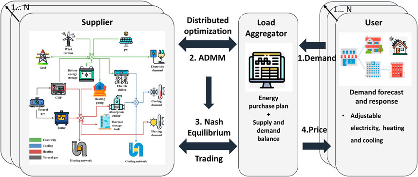
FIGURE 1. Schematic diagram of the holistic method.

The major contributions of this work are summarized as follows.

1)Develop a design and operation optimization method for multi-area IES based on a multi-agent model. The demand response strategy of users and the supply strategy of IES subsystems can be analyzed effectively when considering the overall optimization.

2)Long-term annualized objectives like annual carbon emissions are incorporated into the distributed optimization. The operation of the subsystem is effectively optimized in consideration of long-term benefits.

3)A supply-demand matching approach to energy pricing and profit allocation is established. Energy trading between users and subsystems. The fairness of energy transactions between users and subsystems can be ensured by using this pricing and profit allocation method.

The rest of this paper is organized as follows. Section 2 describes the methods, including the demand response model and distributed optimized model for multi-area IES. Section 3 analyses a simple case to illustrate the process and effectiveness of the model. Section 4 introduces a case study analysis. Section 5 provides results and discussion. Section 6 concludes the whole study.

2 Materials and methods

The detailed process of the proposed method is shown in Figure 2. Firstly, the energy demand of different residential, industrial and commercial users in the planning area are forecasted and used as input parameters for the demand response model and the multi-objective optimization model for IES. Subsequently, the planning of each subsystem of the multi-area IES is optimized separately, with cost and carbon emission as optimization objectives. The demand response model, distributed optimization model for IES, and profit allocation method are cyclic optimization processes. The initial energy price is input into the demand response model, and the calculated energy demand at the price is input into the distributed optimization model for IES. The energy supply at the price is fed back to the demand response model. At the same time, the benefits of subsystems and users are input into the profit allocation method to evaluate the fairness of the profit allocation at the current price. If the optimal price is not reached, the new price is generated by systematic sampling within the feasible range and input into the demand response model and distributed optimization model for IES again.

FIGURE 2

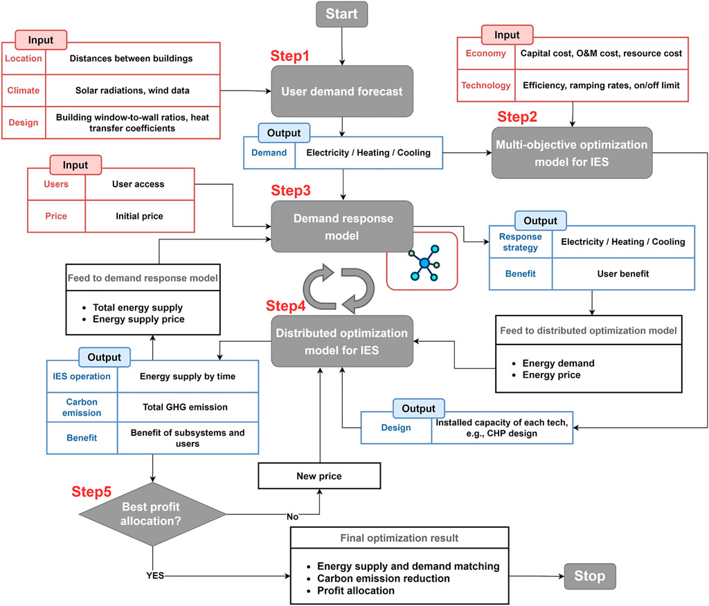
FIGURE 2. The process diagram of the proposed method.

2.1 Demand forecast method

Tools for forecasting demand in urban areas include SUNtool, CitySIM, CityBES, City Energy Analyst (CEA), etc. (Johari et al., 2020) The forecasting accuracy of CEA has been evaluated and compared with empirical data and the output of CLM–EnergyPlus, and the result showed high reliability (Fonseca and Schlueter, 2015). In this study, CEA (ETH Zurich, 2022) is used to forecast the hourly energy demand of each user in a typical year for urban areas. This tool is based on spatial analysis and dynamic building energy modeling, and the input parameters include weather data and building design information.

Considering the scale of the model, introducing year-round hourly data (including renewable resources and energy demand, 8760 h) into the optimization can create a large number of variables and constraints, which can lead to high-dimensional problems and unacceptable computational costs. In addition, since the supply side is a system model with large granularity, the feature extraction of energy demand, and identifying an appropriate number of typical demands can solve the supply and demand side matching problem. To ensure the model calculation speed, typical daily data and occurrence probability instead of year-round hourly data are introduced into the proposed optimization model. In order to generate enough typical scenarios to represent the fluctuation of the energy demand curve, the K-Medoids clustering method (Arora et al., 2016) is introduced. The process of the K-Medoids clustering method shows as follows.

First, k daily energy demands are selected as the cluster center points in all samples. Second, calculate the Euclidean distance between the remaining points and the center points, and assign the remaining points to the clusters represented by the current closest center point according to the principle of being closest to the center point. Then, for the other points in each cluster except the center point, when calculating the point as the new center point, the sum of the distances from all other points to the center point is calculated, and the point corresponding to the minimum total distance is selected as the new center point. Finally, the second and third steps are repeated until all the center points no longer change or the maximum number of iterations is reached, and the center point at this time is used as the clustering result.

2.2 User demand response model

The user in this study is modeled as a rational agent that can regulate its own energy demand. The regulating behavior of users includes shifting electricity demand from peak tariff periods to off-peak tariff periods and curtailing heating or cooling demand appropriately during peak times. The electricity, heating, and cooling response strategy of users is shown in Eqs 1a–e. The users try to maximize their own benefits, and the energy demand is determined by the difference between energy consumption satisfaction ($V_i\left(E_{t,i,s,h}\right)$) and energy consumption cost ($C_i\left(E_{t,i,s,h}\right)$) (Wang et al., 2021), as shown in Eq. 1a. Energy consumption satisfaction is a function of the user’s energy consumption ($E_{t,i,s,h}$), and the form of this function is usually quadratic or logarithmic (Khorasany et al., 2021). In this study, the quadratic form is used, as shown in Eq. 1b. Energy consumption cost depends on energy consumption and energy prices, as shown in Eq. 1c. Eq. 1d represents the range of values of user demand, which are determined by the user’s energy-using equipment and energy-using habits. The non-reducible but transferable electricity demand is bounded by Eq. 1e, and the ratio of non-reducible demand to total demand tends to be one for residential users, or between 0.95 and 0.97 for commercial and industrial users. After the response process, users submit their energy demand to the LA. On behalf of users, LA directly participates in the coordinated optimization with the suppliers. Users purchase energy at the hourly agreed energy price between LA and subsystems.

$E_{t,i,s,h}=arg\mathit{max}\left[V_i\left(E_{t,i,s,h}\right)-C_i\left(E_{t,i,s,h}\right)\right],\forall i\in I,\forall s\in S,\forall h\in H,\forall t\in \left\{el,he,co\right\}(\mathrm{1a})$

$V_i\left(E_{t,i,s,h}\right)={\sum }_{t,s,h}\left(-\frac{\mathit{1}}{\mathit{2}}{{\alpha }_{t,i,s,h}E}_{t,i,s,h}^{\mathit{2}}+{\beta }_{t,i,s,h}{E}_{t,i,s,h}\right),\forall i\in I,t\in \left\{el,he,co\right\}(\mathrm{1b})$

$C_i\left(E_{t,i,s,h}\right)={\sum }_{t,s,h}{p}_{t,i,s,h}{E}_{t,i,s,h},\forall i\in I,t\in \left\{el,he,co\right\}(\mathrm{1c})$

${\underset{¯}{E}}_{t,i,s,h}\le E_{t,i,s,h}\le {\overline{E}}_{t,i,s,h},\forall i\in I,\forall s\in S,\forall h\in H,\forall t\in \left\{el,he,co\right\}(\mathrm{1d})$

${\sum }_h{E}_{el,i,s,h}\ge {\gamma }_{i,nc}{\sum }_h{E}_{el,i,s,h}^{total-demand},\forall i\in I,\forall s\in S(1e)$

where $I$ represents users, $S$ and $H$ represent typical days and hours in the daytime, respectively. $t$ includes electricity, heating, and cooling. ${\alpha }_{t,i,s,h}$ and ${\beta }_{t,i,s,h}$ denote the time-dependent parameters that are determined by user energy consumption, $p_{t,i,s,h}$ represents the energy price, ${\underset{¯}{E}}_{t,i,s,h}$ represents the minimum acceptable user demand, ${\overline{E}}_{t,i,s,h}$ represents the maximum acceptable demand, ${\gamma }_{i,nc}$ denotes the ratio of non-reducible electricity demand to the overall electricity demand, and $E_{el,i,s,h}^{total-demand}$ denotes the overall electricity demand.

2.3 Distributed optimization method for multi-area integrated energy systems

In this model, the subsystems of multi-area IES which are connected with the grid, heating, and cooling network are used as suppliers. Each subsystem is modeled as a rational agent, and mainly includes energy facilities such as CHP units, boilers, heat pumps, electric chillers, absorption chillers, battery energy storage, thermal storage tank, and renewable energy facilities such as PV and wind turbines. The MILP (Mixed Integer Linear Programming) method is adopted to optimize technology selection, installed capacity, and system scheduling with the balance of carbon emission and cost (Zhang et al., 2019). During the operation stage, each subsystem regulates its own operation strategies and shares information about the exchanged energy flows and carbon emissions.

2.3.1 Multi-objective optimization for integrated energy systems

In order to determine the optimal capacity for each subsystem of the multi-area IES, the annual total cost (ATC) and annual carbon emission (ACE) are chosen as optimization objectives. The available technology options of IES are shown in Figure 3. ATC includes the capital expenditure (CAPEX), the fuel cost (FC), and the maintenance cost (MC), as shown in Eq. 2. ACE comes from external electricity and natural gas consumed by the system, as shown in Eq. 3. In addition, CAPEX includes the capital costs of pipelines and other energy technologies, as calculated in Eq. 4. Eq. 5 shows the calculation of the capital recovery factor (CRF). FC and MC are related to the output of different technologies as determined by Eqs 6, 7, respectively.

${Obj}_n^{cost}={CAPEX}_n\times CRF+{\sum }_{s,h}{prob}_s\times \left(F{C}_{n,s,h}+M{C}_{n,s,h}\right),\forall n\in N(2)$

$Ob{j}_n^{emi}={\sum }_{s,h}pro{b}_s\times \left[em{i}_{s,h}^{elec-im}\times E_{n,s,h}^{elec-im}+em{i}_{s,h}^{NG}\times \left(\frac{E_{n,s,h}^{CHP}}{{\eta }_{CHP}}+\frac{Q_{n,s,h}^{b-heat}}{{\eta }_b}\right)\right],\forall n\in N(3)$

${CAPEX}_n={\sum }_{pipe}{LP}_{n,pipe}\times C_{pipe}^{CAP}+{\sum }_{tech}{CAP}_{n,tech}\times C_{tech}^{CAP},\forall n\in N(4)$

$CRF=\frac{r\times {\left(\mathrm{1}+r\right)}^y}{{\left(\mathrm{1}+r\right)}^y-\mathrm{1}},(5)$

$F{C}_{n,s,h}=\left(\frac{E_{n,s,h}^{CHP}}{{\eta }_{CHP}}+\frac{Q_{n,s,h}^{b-heat}}{{\eta }_b}\right)\times C^{NG}+E_{n,s,h}^{elec-im}\times C_h^{elec-im},\forall n\in N,\forall s\in S,\forall h\in H(6)$

$M{C}_{n,s,h}=E_{n,s,h}^{CHP}\times C_{CHP}^M+Q_{n,s,h}^{b-heat}\times C_b^M+Q_{n,s,h}^{HP}\times C_{HP}^M+Q_{n,s,h}^{ec-cool}\times C_{ec}^M+Q_{n,s,h}^{ac-cool}\times C_{ac}^M+E_{n,s,h}^{WT}\times C_{WT}^M+E_{n,s,h}^{PV}\times C_{PV}^M+E_{n,s,h}^{est-char}\times C_{est}^M+Q_{n,s,h}^{hst-char}\times C_{hst}^M,\forall n\in N,\forall s\in S,\forall h\in H(7)$

where $N$ represents suppliers, i.e., the subsystems, ${prob}_s$ is the probability of each typical day, the subscripts of $pipe$ and $tech$ represent the different types of pipelines and IES technologies, respectively. ${CAP}_{n,tech}$ represents the installed capacity, ${LP}_{n,pipe}$ is the length of the pipeline, $C_{pipe}^{CAP}$ and $C_{tech}^{CAP}$ represent the unit cost of pipeline and IES technologies, respectively. $r$ is the interest rate and is considered as 6% (Jing et al., 2017), $y$ represents the project life in years, $C^{NG}$ represents the unit cost of nature gas, $C_h^{elec-im}$ represents the unit cost of electricity from grid, and $C^M$ represents the unit maintenance cost of different technology.

FIGURE 3

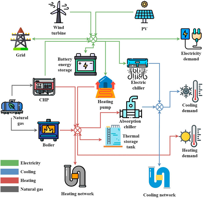
FIGURE 3. Available technology options of subsystems.

For equipment such as battery energy storage, operation-dependent degradation cost and lifespan reduction would impact the availability and economics of IES. In this model, regular replenishment of the battery modules according to the degree of degradation is considered to ensure stable performance of the battery energy storage. The degradation cost of battery energy storage is discounted in the maintenance cost associated with the operation. In addition to battery energy storage, other equipment without significant degradation is planned with redundant capacity so that the remaining capacity after degradation could meet the operation requirements.

The lifespan of the battery energy storage is calculated according to $Life=\frac{C^{F_{100}}}{{\sum }_{a,d}\frac{1}{2}{D}_{a,d}^{kp}}$ (Kazemi and Zareipour, 2018), where $C^{F_{\mathit{100}}}$ represents the maximum number of full charge-discharge, $D_{a,d}$ represents the depth of the $a$ th charge/discharge on day $d$, and $kp$ is a constant in the range of 0.8–2.1. Lowering the depth of charge/discharge and reducing the daily times of charge/discharge can effectively improve the battery lifespan. When the lifespan is lower than the program lifetime, the battery energy storage needs to be replaced. Lifespan reduction of other equipment is not significant. With regular maintenance and avoiding drastic power changes, CHP units usually would not require replacement over a project life of about 20 years.

There is a trade-off between the ATC and ACE of multi-objective optimization, and there is no guarantee that both are optimal at the same time. The trade-off between conflicting objectives can be clearly seen by generating the Pareto Frontier. In this study, the $\epsilon$-constraint (Zhang et al., 2015) is used to solve the bi-objective optimization. The constraint approach keeps one of the objectives, such as ATC, as the objective function and transforms the other objective, such as ACE, into the constraint. The constraint ACE ≤ $\epsilon$ is added to the model by introducing a parameter $\epsilon$. Thus, the bi-objective optimization is transformed into a single-objective optimization. By minimizing ATC and ACE respectively, the values of maximum ${ACE}^{\mathit{max}}$ and minimum ${ACE}^{\mathit{min}}$ of ACE can be obtained. Then, for each N+1 point, the value of $\epsilon$ is calculated by ${ACE}^{\mathit{max}}-\frac{{ACE}^{\mathit{max}}-{ACE}^{\mathit{min}}}{N}\delta$, where N is the user-defined number of intervals between ${ACE}^{\mathit{max}}$ and ${ACE}^{\mathit{min}}$, $\delta$ = 1, 2, ..., N. The specific description of the ε-constraint constraint for solving the multi-objective problem can be found in (Zhang et al., 2015), which is not discussed in detail in this paper.

In order to determine the optimal solution from multiple solutions on the Pareto frontiers, Euclidean distance-based decision-making methods can be adopted. These methods determine the optimal solution by calculating the Euclidean distance from each solution to the ideal point and the nadir point after normalizing the value of the objective function. Linear Programming Techniques for Multidimensional Analysis of Preference (LINMAP) selects the solution with the minimum distance from the ideal point as the optimal solution, while Technique for Order Preference by Similarity to an Ideal Solution (TOPSIS) selects the solution with the largest ratio of the distance from the ideal point to distance from the nadir point as the optimal solution. In addition to the Euclidean distance-based methods, Shannon’s entropy-based methods and fuzzy theory-based methods are also commonly used, which can be referred to (Jing et al., 2018) for details.

2.3.2 Supply balance for subsystems of integrated energy systems

The electricity, heating, and cooling supply of the subsystem mainly depends on the output of each technology. The electricity supply ($E_{n,s,h}^{el,sup}$) is calculated by Eq. 8 which includes electricity production from CHP unit ($E_{n,s,h}^{CHP}$), grid ($E_{n,s,h}^{im}$), PV($E_{n,s,h}^{PV}$) and wind turbine ($E_{n,s,h}^{WT}$), electricity consumption from heat pump ($E_{n,s,h}^{HP}$) and electric chiller ($E_{n,s,h}^{\mathrm{e}\mathrm{c}}$), the charged ($E_{n,s,h}^{est-char}$) and discharged ($E_{n,s,h}^{est-disc}$) electricity of battery energy storage, as well as input electricity ($E_{m,n,s,h}^{el,in}$) and output electricity ($E_{n,m,s,h}^{el,out}$). The heating supply ($Q_{n,s,h}^{he,sup}$) is calculated by Eq. 9, where the heating supply is equal to the sum of the CHP unit heating output $(Q_{n,s,h}^{CHP-heat}$), boiler heating output ($Q_{n,s,h}^{b-heat}$), storage heating discharged ($Q_{n,s,h}^{hst-disc}$) and the heating input ($Q_{m,n,s,h}^{he,in}$) from other subsystems, minus the storage heating charged ($Q_{n,s,h}^{hst-char}$), the absorption chiller heating input ($Q_{n,s,h}^{ac-heat}$) and the heating output ($Q_{n,m,s,h}^{he,out}$) to other subsystems. Similarly, Eq. 10 describes the cooling supply ($Q_{n,s,h}^{co,sup}$), covering electric chiller cooling output ($Q_{n,s,h}^{ec-cool}$) and absorption chiller cooling output ($Q_{n,s,h}^{ac-cool}$), cooling input ($Q_{m,n,s,h}^{co,in}$) and cooling output ($Q_{n,m,s,h}^{co,out}$). Considering the energy transfer of adjacent subsystems, ${\nu }_{m,n}^{el}$, ${\nu }_{m,n}^{he}$ and ${\nu }_{m,n}^{co}$ represent electricity, heating, and cooling loss factors when transferring energy from subsystem $m$ to adjacent subsystem $n$, respectively.

$E_{n,s,h}^{el,sup}=E_{n,s,h}^{CHP}+E_{n,s,h}^{im}+E_{n,s,h}^{PV}+E_{n,s,h}^{WT}+E_{n,s,h}^{est-disc}-E_{n,s,h}^{est-char}-E_{n,s,h}^{HP}-E_{n,s,h}^{ec}+{\displaystyle \sum }_{m\ne n}{\nu }_{m,n}^{el}{E}_{m,n,s,h}^{el,in}-{\displaystyle \sum }_{m\ne n}{\nu }_{n,m}^{el}{E}_{n,m,s,h}^{el,out},\forall m\in N,\forall n\in N,\forall s\in S,\forall h\in H(8)$

$Q_{n,s,h}^{he,sup}=Q_{n,s,h}^{CHP-heat}+Q_{n,s,h}^{b-heat}+Q_{n,s,h}^{HP-heat}+Q_{n,s,h}^{hst-disc}{-Q}_{n,s,h}^{hst-char}{-Q}_{n,s,h}^{ac-heat}+{\displaystyle \sum }_{m\ne n}{\nu }_{m,n}^{he}{Q}_{m,n,s,h}^{he,in}-{\displaystyle \sum }_{m\ne n}{\nu }_{n,m}^{he}{Q}_{n,m,s,h}^{he,out},\forall m\in N,\forall n\in N,\forall s\in S,\forall h\in H(9)$

$Q_{n,s,h}^{co,sup}=Q_{n,s,h}^{ec-cool}+Q_{n,s,h}^{ac-cool}+{\displaystyle \sum }_{m\ne n}{\nu }_{m,n}^{co}{Q}_{m,n,s,h}^{co,in}-{\displaystyle \sum }_{m\ne n}{\nu }_{n,m}^{co}{Q}_{n,m,s,h}^{co,out},\forall m\in N,\forall n\in N,\forall s\in S,\forall h\in H(10)$

The detailed technology constraints can be found in Section 2.3.3.

2.3.3 Technology constraints

This section provides detailed technology constraints of the optimization model for IES.

The energy output of the device cannot exceed its installed capacity, which can be defined as

$E_{n,s,h}^{CHP}\le {CAP}_n^{CHP}\times {TI}_h,\forall n,s,h(\mathrm{11a})$

$Q_{n,s,h}^{b-heat}\le {CAP}_n^b\times {TI}_h,\forall n,s,h(\mathrm{11b})$

$Q_{n,s,h}^{HP-heat}\le {CAP}_n^{HP}\times {TI}_h,\forall n,s,h(\mathrm{11c})$

$Q_{n,s,h}^{ec-cool}\le {CAP}_n^{ec}\times {TI}_h,\forall n,s,h(\mathrm{11d})$

$Q_{n,s,h}^{ac-cool}\le {CAP}_n^{ac}\times {TI}_h,\forall n,s,h(11e)$

where ${TI}_h$ denotes each operating step of the time interval.

The energy conversion constraints can be defined as

$Q_{n,s,h}^{b-heat}={\eta }^b\times N{G}_{n,s,h}^b,\forall n,s,h(\mathrm{12a})$

$Q_{n,s,h}^{HP}={\eta }^{HP}\times E_{n,s,h}^{HP},\forall n,s,h(\mathrm{12b})$

$Q_{n,s,h}^{ec-cool}={\eta }^{ec}\times E_{n,s,h}^{ec},\forall n,s,h(\mathrm{12c})$

$Q_{n,s,h}^{ac-cool}={\eta }^{ac}\times Q_{n,s,h}^{ac-cool},\forall n,s,h(\mathrm{12d})$

where $\eta$ represents the device efficiency, and ${NG}^b$ represents the natural gas consumption of the boiler.

In the present study, back-pressure micro gas turbines are chosen as the main equipment for CHP units. This kind of CHP unit has a constant heat to power ratio (${\sigma }_n$) and a minimum power output limit, which can be defined as

$Q_{n,s,h}^{CHP}{⩽\sigma }_n{E}_{n,s,h}^{CHP},\forall n,s,h(\mathrm{13a})$

$E_{n,s,h}^{CHP}⩽\left(1-{\chi }_{n,s,h}^{CHP}\right)\times M_{\mathrm{1},CHP},\forall n,s,h(\mathrm{13b})$

$E_{n,s,h}^{CHP}⩾{\mathrm{0.3}\times CAP}^{CHP}-{\chi }_{n,s,h}^{CHP}\times M_{\mathrm{2},CHP},\forall n,s,h(\mathrm{13c})$

where binary variable ${\chi }_{n,s,h}^{CHP}$ controls the on/off status of the CHP unit, and $M_{\mathit{1},CHP}$ and $M_{\mathit{2},CHP}$ are sufficiently large variables.

The output of renewable energy technologies is calculated based on meteorological resource conditions. For example, the power output of the PV system is calculated by Eqs 14a,b (Lin et al., 2021).

$E_{s,h}^{PV,elec}=N^{m,PV}\times {EA}^{m,PV}\times S{I}_{s,h}\times {\eta }_{s,h}^{PV}\times {TI}_h,\forall s,h(\mathrm{14a})$

$\begin{array}{c}{\eta }_{s,h}^{PV}={\theta }_{\mathrm{0}}^{PV}\times \left[{\left(\frac{S{I}_{s,h}^{PV}}{S{I}_{\mathrm{0}}}\right)}^{{\theta }_{\mathrm{1}}^{PV}}+{\theta }_{\mathrm{2}}^{PV}\times \left(\frac{S{I}_{s,h}^{PV}}{S{I}_{\mathrm{0}}}\right)\right]\\ \times [\mathrm{1}+{\theta }_{\mathrm{3}}^{PV}\times {\left(\frac{T_{s,h}^{PV}}{T_{\mathrm{0}}}\right)}^{{\theta }_{\mathrm{1}}^{PV}}\\ +{\theta }_{\mathrm{4}}^{PV}\times {\left(\frac{A{M}_{s,h}}{A{M}_{\mathrm{0}}}\right)}^{{\theta }_{\mathit{1}}^{PV}}],\forall s,h\end{array}(\mathrm{14b})$

The PV energy output is determined by the incident solar radiation ($S{I}_{s,h}$), the effective area per module (${EA}^{m,PV}$) corrected according to the tilt angle, and the number of modules ($N^{m,PV}$). The empirical parameters ${\theta }_{\mathit{0}}^{PV}$, ${\theta }_{\mathit{1}}^{PV}$, ${\theta }_{\mathit{2}}^{PV}$, ${\theta }_{\mathit{3}}^{PV}$, and ${\theta }_{\mathit{4}}^{PV}$ are determined by the device’s performance. $S{I}_{\mathit{0}}$, $T_{\mathit{0}}$, and $A{M}_{\mathit{0}}$ are the standard values for incident solar radiation, panel temperature, and airmass. These values are listed in Supplementary Table S1 of the supplementary material.

The power output of wind turbines can be calculated as follows,

$E_{s,h}^{WT}=\{\begin{array}{c}\mathrm{0},v_{s,h}<v^{in},v_{s,h}>v^{out}\\ N^{m,WT}\times {AP}_{s,h}^{m,WT}\times {TI}_h,v^{in}\le v_{s,h}<v^{rated},\\ {CAP}^{WT}\times {TI}_h,v^{rated}\le v_{s,h}\le v^{out}\end{array}\forall s,h(\mathrm{15a})$

${AP}_{s,h}^{m,WT}{=\theta }_{\mathrm{3}}^{WT}{v}_{s,h}^{\mathit{3}}+{{\theta }_{\mathrm{2}}^{WT}v}_{s,h}^{\mathrm{2}}+{\theta }_{\mathrm{1}}^{WT}{v}_{s,h}+{\theta }_{\mathrm{0}}^{WT},\forall s,h(\mathrm{15b})$

The output of wind turbines depends mainly on the average wind speed ($v_{s,h}$), as shown in Eq. 15a. The turbine generates electricity only when the real-time wind speed stays within the range of cut-in and cut-out wind speeds, i.e., $v_{s,h}ϵ$[$v^{in}$, $v^{out}$]. $v^{\mathrm{r}\mathrm{a}\mathrm{t}\mathrm{e}\mathrm{d}}$ denotes the rated wind speed. ${CAP}^{WT}$ denotes the total installed capacity, i.e., the sum of the rated power. ${AP}^{m,WT}$ denotes the average power per module. ${TI}_h$ denotes each operating step of the time interval. When the wind speed is between $v^{in}$ and $v^{rated}$, ${AP}^{m,WT}$ can be calculated according to Eq. 15b, where ${\theta }_{\mathit{0}}^{WT}$, ${\theta }_{\mathit{1}}^{WT}$, ${\theta }_{\mathit{2}}^{WT}$, and ${\theta }_{\mathit{3}}^{WT}$ are the fitting parameters as shown in Supplementary Table S1 of the supplementary material.

In terms of energy storage, the amount of energy stored in storage facilities ($E_{t,n,s,h}^{st-in}$) should be smaller than the installed capacity (${CAP}^{st}$), as shown in Eqs 16a,b. $t$ represents the type of energy storage, including electrical storage and thermal storage. ${\eta }_t^{st-char}$, ${\eta }_t^{st-disc}$ and ${\eta }_t^{st-in}$ represent charge, discharge, and storage efficiency, respectively. Meanwhile, Eqs 17a–c is introduced to avoid the simultaneous charging and discharging of the energy storage facilities, where ${\chi }_{t,n,s,h}^{st-disc}$ and ${\chi }_{t,n,s,h}^{st-char}$ represent binary variables, and $M_{\mathit{1},st}$ and $M_{\mathit{2},st}$ represent sufficiently large variables.

$E_{t,n,s,h}^{st-in}={\eta }_t^{st-in}\times E_{t,n,s,h-\mathrm{1}}^{st-in}+{\eta }_t^{st-char}\times E_{t,n,s,h}^{st-char}-\frac{E_{t,n,s,h}^{st-disc}}{{\eta }_t^{st-disc}},\forall n,s,h,\forall t\in \left\{el,he\right\}(\mathrm{16a})$

$E_{t,n,s,h}^{st-in}\le {CAP}_t^{st}\times {TI}_h,\forall n,s,h,\forall t\in \left\{el,he\right\}(\mathrm{16b})$

${\chi }_{t,n,s,h}^{st-disc}+{\chi }_{t,n,s,h}^{st-char}\le \mathrm{1},\forall n,s,h,\forall t\in \left\{el,he\right\}(\mathrm{17a})$

$E_{t,n,s,h}^{st-disc}\le {\chi }_{t,n,s,h}^{st-disc}\times M_{\mathrm{1},st},\forall n,s,h,\forall t\in \left\{el,he\right\}(\mathrm{17b})$

$E_{t,n,s,h}^{st-char}\le {\chi }_{t,n,s,h}^{st-char}\times M_{\mathrm{2},st},\forall n,s,h,\forall t\in \left\{el,he\right\}(\mathrm{17c})$

2.3.4 Distributed optimization method

The distributed optimization for suppliers in this work is based on the ADMM algorithm, and the process of the proposed method is shown in Figure 4. In this section, cost ($ATC$) is used as the optimization objective, and carbon emission ($ACE$) is used as a variable that affects the cost. The cost of supplier (${ATC}_n$) is a function of the energy supply ($E_{n,t,s,h}$) and carbon emission (${ACE}_n$) when the CAPEX is fixed, as shown in Eq. 18. The model can achieve distributed optimization by decomposing the total cost of energy supply into the cost of each supplier, as shown in Eqs 19, 20. Compared to the total objective in Eq. 19, additional Lagrangian residual terms of energy supply and carbon emission are added to the objective of each supplier in the $k$ th iteration (Eq. 20). The carbon emission of each supplier is calculated according to Eq. 21. In order to control the total carbon emission, ensure fairness in the distribution of carbon emission reduction responsibility and avoid monopolization of energy supply by one supplier, the maximum carbon emission of each supplier is determined based on the energy supply and carbon reduction cost of each supplier when operating individually as shown in Eq. 22.

${ATC}_n\left(E_{n,t,s,h},{ACE}_n\right)={CAPEX}_n\times CRF+{\sum }_{s,h}{prob}_s\times \left(F{C}_{n,s,h}\left(E_{n,t,s,h},{ACE}_n\right)+M{C}_{n,s,h}\left(E_{n,t,s,h},{ACE}_n\right)\right),\forall n\in N,E_{n,t,s,h}\in \left\{E_{n,s,h}^{el,sup},Q_{n,s,h}^{he,sup},Q_{n,s,h}^{co,sup}\right\}(18)$

${obj}^{cen}={\sum }_n{ATC}_n\left(E_{n,t,s,h},{ACE}_n\right),\forall s\in S,\forall h\in H,E_{n,t,s,h}\in \left\{E_{n,s,h}^{el,sup},Q_{n,s,h}^{he,sup},Q_{n,s,h}^{co,sup}\right\}(19)$

${obj}_n^{dis,k}={ATC}_n\left(E_{n,t,s,h},{ACE}_n\right)+{\sum }_{t,s,h}\left(\begin{array}{c}{\lambda }_{t,s,h}^k\times \left(E_{t,s,h}^{tot}-{\displaystyle \sum }_{m\ne n}{E}_{m,t,s,h}^{k-\mathrm{1}}-E_{n,t,s,h}\right)\\ +\frac{{\rho }_t^k}{\mathrm{2}}{\times \parallel E_{t,s,h}^{tot}-{\displaystyle \sum }_{m\ne n}{E}_{m,t,s,h}^{k-\mathrm{1}}-E_{n,t,s,h}\parallel }_{\mathrm{2}}^{\mathrm{2}}\end{array}\right)+\left(\begin{array}{c}{\lambda }_{emi}^k\times \left({ACE}^{tot}-{\displaystyle \sum }_{m\ne n}{ACE}_m^{k-\mathrm{1}}-{ACE}_n\right)\\ +\frac{{\rho }_{emi}^k}{\mathrm{2}}{\times \parallel {ACE}^{tot}-{\displaystyle \sum }_{m\ne n}{ACE}_m^{k-\mathrm{1}}-{ACE}_n\parallel }_{\mathrm{2}}^{\mathrm{2}}\end{array}\right),\forall k\in K,\forall n\in N,m\in N{,E}_{n,t,s,h}\in \left\{E_{n,s,h}^{el,sup},Q_{n,s,h}^{he,sup},Q_{n,s,h}^{co,sup}\right\}(20)$

${ACE}_n={\sum }_{s,h}pro{b}_s\times \left(em{i}_{s,h}^{elec-im}\times E_{n,s,h}^{elec-im}+em{i}_{s,h}^{NG}\times \left(\frac{E_{n,s,h}^{CHP}}{{\eta }_{CHP}}+\frac{Q_{n,s,h}^{b-heat}}{{\eta }_b}\right)\right),\forall n\in N(21)$

${ACE}_n\le {\kappa \times \gamma }_{n,carb}\times {ACE}^{tot},\forall n\in N(22)$

where $n$ represents the $n$th supplier, $E_{n,t,s,h}$ contains the supply of electricity ($E_{n,s,h}^{el,sup}$), heating ($Q_{n,s,h}^{he,sup}$) and cooling ($Q_{n,s,h}^{co,sup}$), ${ACE}_n$ represents the carbon emission, $E_{t,s,h}^{tot}$ represents the total energy demand, ${ACE}^{tot}$ represents the total maximum amount of carbon emission, $E_{m,t,s,h}^{k-\mathit{1}}$ and ${ACE}_m^{k-\mathit{1}}$ represent the energy supply and carbon emission of the other suppliers without nth supplier in the $k-\mathit{1}$th iteration, respectively. ${\lambda }_{t,s,h}^k$ and ${\lambda }_{emi}^k$ represent the Lagrangian operator, ${\rho }_t^k$ and ${\rho }_{emi}^k$ represent the penalty factor, ${\gamma }_{n,carb}$ denotes the proportion of carbon emission allocated to each subsystem, and $\kappa$ represents the upper limit of the uplift factor, which is chosen according to the case.

FIGURE 4

FIGURE 4. Distributed optimization flow chart.

The primal residuals and dual residuals of the kth iteration are calculated according to Eqs 23a,b, 24a,b respectively (Boyd et al., 2011).

$r_{t,s,h}^k=E_{t,s,h}^{tot}-{\sum }_n{E}_{n,t,s,h}^k,\forall s\in S,\forall h\in H,\forall t\in \left\{el,he,co\right\}(\mathrm{23a})$

$r_{emi}^k=E_{emi}^{tot}-{\sum }_n{E}_{n,emi}^k,(\mathrm{23b})$

$s_{n,t,s,h}^k=E_{n,t,s,h}^k-E_{n,t,s,h}^{k-\mathrm{1}},\forall n\in N,\forall s\in S,\forall h\in H,\forall t\in \left\{el,he,co\right\}(\mathrm{24a})$

$s_{n,emi}^k=E_{n,emi}^k-E_{n,emi}^{k-\mathrm{1}},\forall n\in N(\mathrm{24b})$

In each iteration, the Lagrangian operator (${\lambda }^k$) is updated according to Eqs 25a,b. In order to improve the convergence and make the performance less dependent on the initial choice of the penalty parameter, the varying penalty parameter proposed by Boyd et al. (2011) is adopted, and the penalty factor (${\rho }^k$) is updated as shown in Eqs 26a–f in each iteration. In general, $\mu$ is taken as 10 and ${\tau }^{incr}$ and ${\tau }^{decr}$ are taken as 2.

${\lambda }_{t,s,h}^k={\lambda }_{t,s,h}^{k-\mathrm{1}}+{\rho }_t^k{r}_{t,s,h}^k,\forall s\in S,\forall h\in H,\forall t\in \left\{el,he,co\right\}(\mathrm{25a})$

${\lambda }_{emi}^k={\lambda }_{emi}^{k-\mathit{1}}+{\rho }_{emi}^k{r}_{emi}^k,(\mathrm{25b})$

${\rho }_t^{k+\mathrm{1}}=\{\begin{array}{c}{\tau }^{incr}{\rho }_t^k,r_t^{tot,k}>\mu s_t^{tot,k}\\ {\rho }_t^k/{\tau }^{decr},s_t^{tot,k}>\mu r_t^{tot,k}\\ {\rho }_t^k,\mathrm{o}\mathrm{t}\mathrm{h}\mathrm{e}\mathrm{r}\end{array},\forall t\in \left\{el,he,co\right\}(\mathrm{26a})$

${\rho }_{emi}^{k+\mathrm{1}}=\{\begin{array}{c}{\tau }^{incr}{\rho }_{emi}^k,r_{emi}^{tot,k}>\mu s_{emi}^{tot,k}\\ {\rho }_{emi}^k/{\tau }^{decr},s_{emi}^{tot,k}>\mu r_{emi}^{tot,k}\\ {\rho }_{emi}^k,\mathrm{o}\mathrm{t}\mathrm{h}\mathrm{e}\mathrm{r}\end{array}(\mathrm{26b})$

$r_t^{tot,k}={\sum }_{s,h}\left|r_{t,s,h}^k\right|,\forall t\in \left\{el,he,co\right\}(\mathrm{26c})$

$r_{emi}^{tot,k}=\left|r_{emi}^k\right|,(\mathrm{26d})$

$s_t^{tot,k}=\frac{{\sum }_{n,s,h}\left|s_{n,t,s,h}^k\right|}{Num},\forall t\in \left\{el,he,co\right\}(26e)$

$s_{emi}^{tot,k}=\frac{{\sum }_n\left|s_{n,emi}^k\right|}{Num},(\mathrm{26f})$

The model is judged to have converged when both the primal residuals and the dual residuals are less than the stopping tolerance, as shown in Eqs 27a,b, 28a,b.

$\left|r_{t,s,h}^k\right|\le {\epsilon }_r,\forall s\in S,\forall h\in H,\forall t\in \left\{el,he,co\right\}(\mathrm{27a})$

$\left|r_{emi}^k\right|\le {\epsilon }_r,(\mathrm{27b})$

$\left|s_{n,t,s,h}^k\right|\le {\epsilon }_s,\forall s\in S,\forall h\in H,\forall t\in \left\{el,he,co\right\}(\mathrm{28a})$

${|s}_{emi}^k|\le {\epsilon }_s,(\mathrm{28b})$

Some designs of the model are described below.

In terms of fairness, the maximum carbon emissions of each subsystem are set based on a weighted average of each subsystem’s annual energy supply and carbon reduction costs as a percentage of the total. The data on annual energy supply and carbon reduction costs comes from the design of multi-objective optimization. On the one hand, subsystems with more annual energy supply have a greater supply capacity and tend to supply more energy in distributed optimization. On the other hand, subsystems with more carbon reduction costs, are often equipped with more costly low-carbon technology equipment, such as wind turbines. The maximum carbon emission can be appropriately increased so that they can supply more energy to obtain more profits when supplying renewable energy. For IES with CHP as the core equipment, the higher carbon emissions usually mean more energy supply and more profits. The fairness guarantee is based on the principle that environment-friendly subsystems with greater supply capacity can have higher rewards.

Since binary variables can affect the convergence of ADMM, in this study, an iterative ADMM method has been proposed, and the binary variables such as the on/off status of the devices of the subsystems are updated iteratively. Before each distributed optimization, each subsystem first performs a pre-optimization individually based on the energy demand of each area to determine the on/off status of the devices and set them as the initial values. In this way, the binary variables are fixed with determined values, and the convexity of the objective function and the convergence of the ADMM are guaranteed. After convergence is reached in one iteration, the binary variables are adjusted and the next iteration of optimization is performed for the operation of the multi-area IES.

In addition to pre-optimization to determine the initial values as well as the varying penalty parameter, appropriate parameter selection can also accelerate the convergence, which is discussed in Section 5.5.

2.4 Profit allocation model

The profit allocation method proposed in this study considers the fairness of profit allocation while maximizing the overall benefit. The profits of different suppliers, LAs, and users, are defined by Eqs 29a–c, respectively. The price is determined by the agreement between LAs and suppliers. The objective function in Eq. 30a represents the centralized planning that maximizes the sum of profits of all users and suppliers, which may lead to an unfair profit allocation. To solve this problem, a Nash-type objective function based on the cooperative game theory proposed by Jing et al. (2021) is adopted, as shown in Eq. 30b. This function leads to a bargaining solution, which fulfills axioms including Individual Rationality, Feasibility, Pareto Optimality, Independence of Irrelevant Alternatives, Independence of Linear Transformations, and Symmetry. The last three axioms ensure the fairness of the bargaining solution (Wang and Huang, 2018). The outputs of the model include 1) the agreed prices for electricity, heating, and cooling, 2) the transaction volumes for different time periods, and 3) the total profits and profit allocation for each participant.

${\pi }_{n,supplier}={\sum }_{t,s,h}{price}_{n,t,s,h}\times E_{n,t,s,h}-{Cost}_n^{supplier},\forall n\in N(\mathrm{29a})$

${\pi }_{LA}={\sum }_{t,s,h}\left({price}_{t,s,h}^u-{price}_{t,s,h}^{agreed}\right)\times E_{t,s,h}^{agg},(\mathrm{29b})$

${\pi }_{i,user}={\sum }_{t,s,h}\left({price}_{t,s,h}^u-{price}_{t,s,h}^{agreed}\right)\times E_{i,t,s,h},\forall i\in I(\mathrm{29c})$

${obj}^{cen}={\sum }_n{\pi }_{n,supplier}+{\pi }_{LA}(\mathrm{30a})$

$\underset{n}{{obj}^{Nash-type}=\prod }\left({\pi }_{n,supplier}-{\pi }_{n,supplier}^{\mathrm{L}}\right)\left({\pi }_{LA}-{\pi }_{LA}^{\mathrm{L}}\right)(\mathrm{30b})$

where ${price}_{t,s,h}^u$ denotes the price of electricity purchased by users from the grid, the price of heating energy from gas boilers, and the price of cooling energy from electric chillers. ${price}_{t,s,h}^{agreed}$ denotes the agreed price between the suppliers and load aggregators, $E_{n,t,s,h},E_{i,t,s,h}$ and $E_{t,s,h}^{agg}$ denote the energy supply of the nth supplier, the energy demand of the $i$th user, and the aggregated demand of the load aggregator ($agg$), respectively. Superscript $L$ denotes the lower bound, ${\pi }_{n,supplier}^{\mathrm{L}}$ and ${\pi }_{LA}^{\mathrm{L}}$ denote the profit when the suppliers and load aggregator do not participate in the coordination, respectively.

Energy prices are obtained through systematic sampling in the price range where ${\pi }_{n,supplier}$, ${\pi }_{LA}$ and ${\pi }_{i,user}$ are all positive. In order to evaluate the fairness of different pricing, with reference to Eq. 30b, the fairness factor ${\omega }_{fair}$ is defined as

$\underset{n}{{\omega }_{fair}=\prod }\left({\pi }_{n,supplier}-{\pi }_{n,supplier}^{\mathrm{L}}\right)\left({\pi }_{LA}-{\pi }_{LA}^{\mathrm{L}}\right)(31)$

3 Case study 1

To illustrate the process and effectiveness of the model, a simple case consisting of an industrial user and two identical subsystems of IES is analyzed in this section. First, the annual demand of the user is obtained by the demand forecasting method, and the energy demand of different seasons is obtained by the clustering method, where the electricity demand of a typical day is shown in Figure 5A. In the figure, the Without DR scenario indicates the demand curve when the user does not participate in the demand response, the moderate response strategy when the price of the Mild DR scenario is lower than the grid price, and the aggressive response strategy when the price of Radical DR is equal to the grid price. Two identical subsystems of IES (SIES) are planned based on typical daily demand. In terms of operation optimization, the energy output by the device for the typical demand shown in Figure 5A is shown in Figure 5B and Figure 5C. Figure 5B shows the scenario with no carbon emission control and Figure 5C shows the scenario with maximum carbon emission. Since electricity from the grid has a higher carbon emission, more electricity is generated by CHP in the scenario of Figure 5C than in the scenario of Figure 5B, and the daily carbon emission is reduced by 15.80%. This demonstrates the effectiveness of using maximum carbon emission in operation optimization.

FIGURE 5

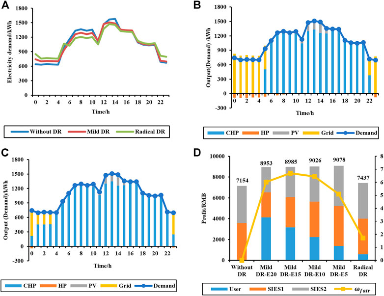
FIGURE 5. The demand curve of different demand strategies in a typical day (A), the energy output of the different devices with no carbon emission control (B) and maximum carbon emission (C), profit of users and SIESs in different scenarios (D).

To analyze the effectiveness of the demand response and profit allocation methods, the Radical DR scenario with no profit allocation and high electricity prices, the Mild DR scenario with profit allocation and moderate electricity prices, and the Without DR scenario are compared. Setting the electricity cost of IES is 0.4 RMB/kWh during the valley hours. Of the day and 0.6 RMB/kWh for peak and normal hours, only 80% of the demand will be purchased from the IES when IES has no price advantage. For Mild DR, the scenarios when the agreed price decreases by 0.05–0.20 RMB/kWh compared to the grid price during the peak and normal hours are analyzed. The daily profits of users and SIES are shown in Figure 5D, and the analysis shows as follows.

When only demand response is considered without profit allocation, users may purchase electricity from the grid, and use gas boilers and electric chillers for heating and cooling because IES has no price advantage. Since the energy conversion efficiency of these approaches is lower than that of IES, the total carbon emissions may be higher. On the other hand, due to higher peak prices, users will adopt more aggressive demand response strategies to reduce energy demand or change their habits to increase demand in the valley in order to save costs. This is a lose-lose situation for both the integrated energy system and the user.

When only profit allocation is considered, users cannot regulate energy demand, and energy demand does not adjust with price changes, resulting in lower bargaining ability.

By comparing different Mild DR scenarios, a trade-off is presented between total profit and fairness. As the electricity price decreases, the profit of users increases, the profit of SIESs decreases, the fairness increases, and the total profit slightly decreases. The reason for this trend is that as the price of electricity decreases, users tend to adopt a relatively moderate demand response strategy, and the rise in electricity demand during peak hours leads to a slight increase in the total cost of energy supply for SIESs. Compared to the “Mild DR-E5” scenario with the electricity price reduction of 0.05 RMB/kWh, the cost of the “Mild DR-E15” with the highest fairness factor increases by 1.02%. And in the “Mild DR-E20” scenario with the electricity price reduction of 0.20 RMB/kWh, the fairness decreases due to the high profit of users. The impact of fairness on trading is greater in this case study, and the price at the peak of fairness is preferred in trade-off decisions. When the agreed price has a large impact on both total profit and fairness, some multi-objective decision-making methods like Euclidean distance-based methods and Shannon’s entropy-based methods (Jing et al., 2018) can be used to obtain the optimal trade-off solution.

4 Case study 2

In order to illustrate how this approach works and to verify the proposed distributed optimization method, a case study has been investigated in an urban district including residential, commercial, and industrial areas located in Weifang, Shandong Province, China. The local climate is cold in winter and hot in summer (Building Energy Research Center of Tsinghua University, 2010). In this case, cooling demand exists only in summer, while heating demand is required only in winter. According to the energy demand, the whole year is divided into three typical seasons, i.e., summer, winter, and transition season.

The energy demand for the whole year is calculated by a tool called CEA (ETH Zurich, 2022). The simulated district is located in the cold region of China, and the meteorological data comes from the region database from EnergyPlus (EnergyPlus, 2022). The total covered area of the district is 31,206 m², where 28 buildings are distributed in different areas, as listed in Supplementary Table S2 of the supplementary material. The energy demand model of buildings is developed based on the methodology provided by Fonseca (2016).

The parameters of residential building envelopes are as follows. 1) The heat transfer coefficients of the roof and exterior walls are considered as 0.66 W/(m²·K) and 0.75 W/(m²·K), respectively. 2) The window-to-wall ratios are set as 0.32 for southward, 0.27 for northward, 0.18 for eastward, and 0.18 for westward. 3) The heat transfer coefficients and solar heat gain coefficient for windows are set as 3.1 W/(m²·K) and 0.6, respectively. These building planning and location information will be used as input of the CEA tool, based on which the hourly electricity, heating, and cooling demands can be obtained.

A subsystem of IES is built in each residential, commercial, and industrial area. Technical and economic parameters are used as inputs of the optimization model to determine the installed capacity of the energy equipment. The major technical parameters are listed in Supplementary Table S3 (Li et al., 2016; Wang et al., 2020) of the supplementary material. The major economic parameters, such as energy prices, unit capital, and maintenance costs, are listed in Supplementary Table S4 (Wang et al., 2020) of the supplementary material. In the baseline scenario, users purchase electricity from the grid at the hourly prices listed in Supplementary Table S4 and use their own gas or electric boilers for heating and electric chillers for cooling.

The maximum number of full charge-discharge of the battery is set to 5,000, the maximum depth of discharge/charge is set to 80%, the maximum daily times of charge/discharge is set to 2, and the life of the storage battery is 20.47 years, which is longer than the program lifetime, so in this case study, the battery would not require replacement during the program life. The operation-related maintenance cost of battery energy storage is 0.095 RMB/kWh including 0.072 RMB/kWh for degradation and 0.023 RMB/kWh for others.

All modeling and optimization procedures are performed on an Intel(R) Core (TM) i7-9700 3.00 GHz PC with 16 GB RAM. The building energy demand is calculated by CEA (ETH Zurich, 2022) tool. The distributed optimization model is developed with Python Pyomo 5.6.9 (Hart et al., 2017) and solved by GAMS (Brooke et al., 1998) with CPLEX (CPLEX, 2019) solver. Influenced by the initial value of optimization and the selection of the device opening and closing states, the CPU times range from 4 to 8 min and the number of iterations ranges from 35 to 50. The stopping tolerance of primal residuals (${\epsilon }_r$) is set as 0.2 Wh, and the stopping tolerance of dual residuals (${\epsilon }_s$) is set as 0.1 Wh.

5 Results and discussion

5.1 Building demand forecast

The simulated energy demand is compared with the statistical demand data of residential and commercial buildings given by the China Association of Building Energy Efficiency (China Association of Building Energy Efficiency, 2022), and the relative error is within 8%. The error mainly comes from the heating and cooling prediction, because the local area is near the sea and has an oceanic climate, which is characterized by warmer nights in winter and cooler nights in summer.

The demand statistics and typical daily demand are shown in Figure 6. The year is divided into winter, summer, and transition seasons according to heating and cooling conditions. Figures 6(A–C) shows the electricity demand, the heating demand in winter, and the cooling demand in summer during the year, respectively. Electricity demand is concentrated during the daytime and fluctuates in a relatively wide range throughout the year. Heating demand is relatively flat in winter. Cooling demand is concentrated during the daytime due to the cool summer night conditions. The daily demand data are grouped into six typical days according to the K-medoids method, as shown in Table 1. Figures 6(D–F) shows the electricity demand in the transition season, the heating demand in winter, and the cooling demand in summer respectively. The variation in electricity demand on each typical day is mainly influenced by whether the industry is working or not, with peaks occurring around meal time, while the variation in heating and cooling demand is mainly influenced by temperature. The total annual demand calculated from the typical day demand and the probability of occurrence of each typical day, compared with the simulated total demand, shows a difference of -0.89% for total electricity demand, −1.33% for total heat demand, and −3.5% for total cooling demand. On the other hand, the K-Medoids method retains the original hour-by-hour energy demand. Combined with the box plots of the annual demand statistics in Figures 6(A–C), it can be seen that the typical daily demands in Figures 6(D–F) are located near the upper and lower quartiles of the box plots (i.e., Q1 and Q3). Therefore, the typical daily data can describe the volatility of energy demand and can be used for the optimization of IES with a certain degree of confidence.

FIGURE 6

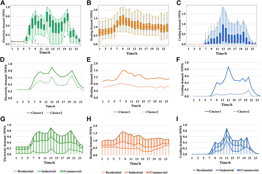
FIGURE 6. Plot of the forecasted energy demand. Figure (A–C) show the annual statistics of hourly electricity, heating, and cooling demand. Hourly electricity demand in the transition season, heating demand in winter, and cooling demand in summer for the typical days are shown in (D–F), respectively. Typical hourly electricity, heating, and cooling demand for cluster one in each region are shown in (G–I).

TABLE 1

TABLE 1. Typical day statistics.

Figures 6(G–I) shows the hour-by-hour demand by area for typical days with higher demand, i.e., cluster 1. In Figure 6G, electricity demand is mainly from the industrial area, with demand concentrated and relatively stable during the daytime. The commercial area has the second highest electricity demand, which is concentrated in the time period of 8–22. Residential area consumes the least electricity, with energy demand concentrated around meal time and night. In Figure 6H, the overall heating demand is relatively stable throughout the day, but the peak hours of energy demand vary by area. The heating demand in residential areas is mainly concentrated in the time of evening and early morning when people are at home and the temperature is lower. While the heating demand of commercial areas is concentrated in the daytime when there is a large stream of people. The cooling demand in summer mainly comes from residential and commercial areas and is concentrated in the daytime, which is influenced by the temperature, as shown in Figure 6I.

5.2 Planning of subsystems of multi-area integrated energy systems

The planning of different subsystems of the multi-area IES is optimized based on the six typical day data extracted in Section 5.1 and the model in Section 2.3.1. The micro gas turbines (MGT) are chosen as the main equipment for the CHP unit. The Pareto frontiers of the planning of subsystems in residential, industrial, and commercial areas are shown in Figures 7A–C, respectively, and the typical planning with different ATC and ACE are shown in Figure 7D and Supplementary Table S5 of the supplementary material. The subsystem of IES built in residential, industrial, and commercial areas are represented by SIES-R (Subsystem of Integrated Energy System in Residential area), SIES-I (Subsystem of Integrated Energy System in Industrial area), and SIES-C (Subsystem of Integrated Energy System in Commercial area), respectively. As shown in Figure 7D, the capacity of absorption chillers and battery energy storage systems increases with the reduction of carbon emission. A2, B2, and C2 are the preference points of TOPSIS (Jing et al., 2019). In order to make sure that the total carbon emission is lower than 35% of the baseline scenario, and to ensure that the total energy supply cost for the three suppliers is lower than 75% of the baseline scenario, A3, B3, and C3 are chosen as the preference points.

FIGURE 7

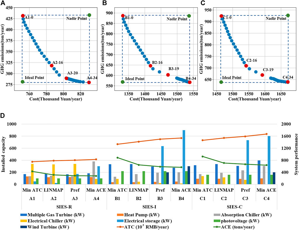
FIGURE 7. The results of the planning optimization of subsystems. Pareto frontiers of subsystem planning in residential, industrial, and commercial areas are shown in (A–C). Figure (D) shows the installed capacity, annual total cost, and annual carbon emission for typical planning.

5.3 Distributed optimization results

Based on the supply and carbon reduction costs as shown in Supplementary Table S5, the maximum amount of carbon emission for subsystems of different areas is determined, and the results are given in Table 2. The upper limit of the uplift factor ($\kappa$ in Eq 22 is set as 5%, i.e., the carbon emission of each subsystem cannot be higher than 105% of the maximum amount of carbon emission in Table 2. Since the total carbon emissions of the three subsystems during the planning phase are no higher than 35% of the baseline scenario, the total amount of carbon emissions is controlled as 35% of the baseline scenario. And according to the energy output of the devices, without maximum carbon emission, the subsystems of IES tend to shut down their CHP systems and purchase electricity from the grid during low tariff hours, with 21.35% of total annual electricity from the grid. With maximum carbon emission, the subsystems tend to supply electricity by CHP during winter and some other low tariff hours to reduce carbon emissions, and the ratio of electricity from the grid decreases to 11.07%. With a 4.87% increase in the cost, a 9.43% reduction in carbon emissions is achieved.

TABLE 2

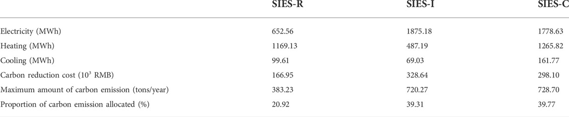
TABLE 2. Annual energy supply and carbon reduction cost.

The profit of the subsystems is defined as the energy sales price minus its cost, and the profit of the load aggregator is calculated as the cost difference between the baseline cost and the purchased energy at the agreed price. The baseline cost is set as the cost of users purchasing electricity from the grid and using their own gas or electric boilers and electric chillers for energy supply. The results of the distributed optimization for each subsystem are shown in Figure 8. The cost reduction of different users at the optimal agreed price is shown in Figure 9. The optimal agreed price for electricity is 0.12 RMB/kWh, lower than the price of grid electricity for peak hours and normal hours, and the optimal agreed price for heating or cooling is 5% lower than the user’s own heating or cooling costs.

FIGURE 8

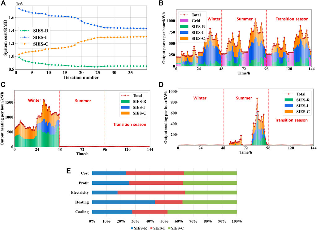
FIGURE 8. The results of distributed optimization for typical days. Figure (A) shows the system cost in the iteration progress. The output electricity, heating, and cooling are shown in (B–D), respectively. Figure (E) shows the output and profit allocation for different IES.

FIGURE 9

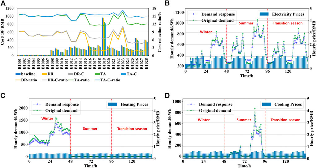
FIGURE 9. The results of demand response of uses. Figure (A) shows the total annual cost and cost reduction ratios for each user under different scenarios. The total electricity, heating, and cooling demand response of users on typical days are shown in (B–D).

After about 40 iterations, the model reaches convergence, and the results are shown in Figure 8A, where the cost of SIES-R and SIES-I decreases as the cost of SIES-C increases. In Figure 8B, during valley tariff periods, electricity is supplied by CHP unit and battery energy storage of subsystem in winter, while in other periods, electricity tends to be purchased from the grid. The reason is that the cost of generating electricity from CHP units is higher than the cost of grid electricity in the valley tariff periods, and the heat generated by CHP units can be used efficiently in winter when heating is required. During the peak tariff periods, electricity is mainly generated by CHP units. In winter, heating energy is mainly provided by SIES-R and SIES-C because the main heating demand comes from residential and commercial areas. The energy output of multi-area IES tends to be flat, and SIES-R provides more electricity and heating during the daytime, compared to the case that traditional energy systems individually supply energy to the area where it is located. Figure 8E shows the ratio of total annual energy supply, cost, and profit for each subsystem. Both SIES-R and SIES-C have a slightly higher profit ratio than their energy cost ratio, as both SIES-R and SIES-C supply more heating and cooling and have higher overall energy supply efficiency.

To further analyze the impact of the coordinated optimization on the energy costs of different users, the energy costs of users under four different scenarios are determined, and the results are shown in Figure 9A. And the scenario setting is shown in Table 3, where DR represents the scenario only considering the demand response of users, and TA represents the scenario in which the subsystem of the multi-area IES transact with users at the optimal agreed price. The DR-C and TA-C scenarios further consider curtailment of electricity demand by industrial and commercial users. According to an assessment of demand response market potential prepared by Environmental Change Institute & Oxford Institute for Energy Studies and University of Oxford (2015), the demand curtailable rate for medium-sized commercial and industrial users is assessed to be between 2% and 7% in 2025. In the case study, the whole day’s electricity demand cuttable ratio is set at 5% for industrial users and 3% for commercial users.

TABLE 3

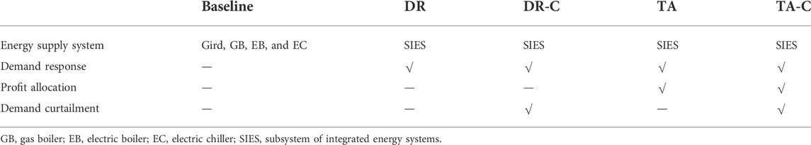
TABLE 3. The scenario setting.

In other words, the energy prices used in the DR and DR-C scenarios are calculated based on purchasing electricity from the grid and using gas or electric boilers and electric chillers for energy supply, while the energy prices used in the TA and TA-C scenarios are the prices with optimal profit allocation. With demand response, users reduce their energy demand during peak periods and increase energy demand during off-peak periods. The total electricity, heating, and cooling demand response are shown in Figures 9(B–D), respectively. In the DR scenario, user cost reduction varies from 3% to 11%, and industrial users have a lower rate of cost reduction because they have less heating demand curtailment. With the further curtailment of electricity demand by industrial and commercial users, the cost reduction rates increase to about 9% for industrial users and about 6% for commercial users in the DR-C scenario. Transaction agreements can significantly reduce costs for users, with a cost reduction ratio ranging from 11% to 16% in the TA scenario. The optimal results are obtained with transaction agreements and electricity demand curtailment by industrial and commercial users, with a cost reduction of 13% or more for all users in the TA-C scenario.

5.4 Price sensitivity analysis

The agreed electricity price derived in the previous section is 0.12 RMB/kWh, which is lower than the grid price during peak and normal hours. The agreed heating and cooling price is 5% lower compared to the user’s own heating and cooling costs. In order to explore the impact of the agreed prices on the participants, this section analyzes the profit allocation for each supplier and the cost reduction for each user at different prices. Figure 10A shows the variation of energy prices with time. The electricity prices are lower than grid prices during peak and normal hours, with reductions ranging from 0.05 to 0.15 RMB/kWh. The heating and cooling prices are lower than the user’s own costs for the whole 24 h, with reductions ranging from 5% to 15% of the user’s own costs. Figure 10B shows the profit allocation at different prices and the fairness factor ${\omega }_{fair}$ in Eqs 30a,b is used to evaluate the fairness of the profit distribution. The different scenarios are named according to the value of the decrease in electricity price and the decreased proportion of heating and cooling price. For example, E05H08C08 represents a 0.05 RMB/kWh decrease in electricity price and an 8% decrease in heating or cooling price. As seen in Figure 10B, the top four scenarios in terms of the fairness factor ${\omega }_{fair}$ show larger reductions in electricity prices and smaller reductions in heating and cooling prices. While high electricity prices lead to an obvious decrease in the fairness factor ${\omega }_{fair}$, scenario E05H08C08 has a significantly lower ${\omega }_{fair}$ than scenario E10H08C08 and scenario E12H08C08. In contrast, high heating and cooling prices lead to a higher ${\omega }_{fair}$, for example, scenario E12H12C12 with higher heating and cooling prices has a higher ${\omega }_{fair}$ than scenario E12H08C08 and scenario E12H05C05. Figure 10C shows the impact of electricity price changes on the cost reduction for different users at a fixed heating and cooling price. It is seen that electricity price reduction has a general effect on cost reduction for all users, and the reductions are higher for industrial users including B1016-B1020, and commercial users including B1024-B1028. It is because these users have higher electricity demand but lower heating and cooling demand. Furthermore, Figure 10D shows the impact of variations in heating and cooling prices on the cost reduction for different users at a fixed electricity price. The influence is greater for residential users including B1001-B1011 and B1014-B1015, as well as for hotel users including B1021-B1023, as these users have higher heating and cooling demand.

FIGURE 10

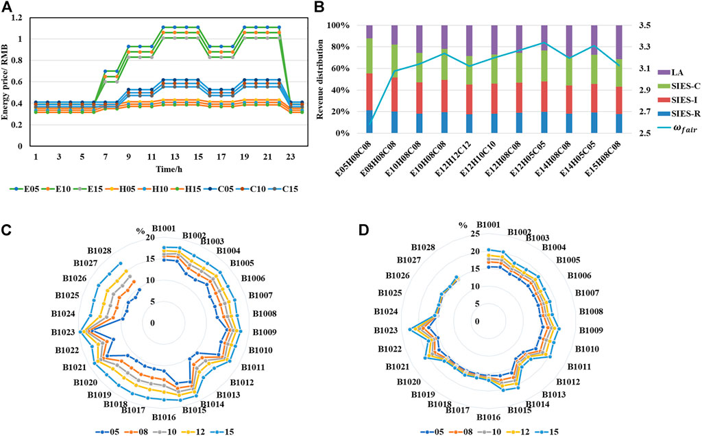
FIGURE 10. The results of the sensitivity analysis of energy prices. Figure (A) shows the variation of energy prices with time. Figure (B) shows the profit distribution between LA and suppliers at various prices. Figure (C) shows the impact of electricity prices on cost reduction by the percentage of different users. Figure (D) shows the impact of heating and cooling prices on cost reduction by the percentage of different users.

5.5 Convergence analysis

In this section, the convergence of the model is investigated. In addition to algorithm design, initial value selection and parameter setting also affect model convergence. The previous section has discussed that the overall optimization performance can be improved and convergence can be achieved faster through the initial value selection and the varying penalty parameter. On the other hand, the accuracy of the result is affected by the stopping tolerance, and the number of iterations can be controlled by using the maximum allowed iterations. Specific parameter values can be selected for each case. Specific parameter values can be selected by considering the case needs, and the influence of the maximum allowed iterations and stopping tolerance is analyzed for the case study.

As described in Section 2.3, the iteration terminates when the stopping condition in Eqs 27a,b, 28a,b is satisfied or when the maximum allowed iterations (K) is reached. The convergence rate of the model depends on the stopping tolerance and maximum allowed iterations. In this study, the stopping tolerance of dual residuals (${\epsilon }_s$) is chosen to be one-half of the stopping tolerance of primal residuals (${\epsilon }_r$). The impact of stopping tolerance for primal residuals (${\epsilon }_r$) on the total cost and the required iteration number are plotted in Figure 11, where the x-axis uses a logarithmic scale with a base of 10. As shown in the figure, when the stopping tolerance is large, e.g., ${\epsilon }_r$>0.1, the stopping tolerance has a considerable impact on the convergence cost. As the stopping tolerance decreases, its impact on the cost gradually decreases. When the stopping tolerance is small enough, e.g., ${\epsilon }_r$<0.01, the impact of stopping tolerance on the cost is negligible, but convergence requires a large number of iterations.

FIGURE 11

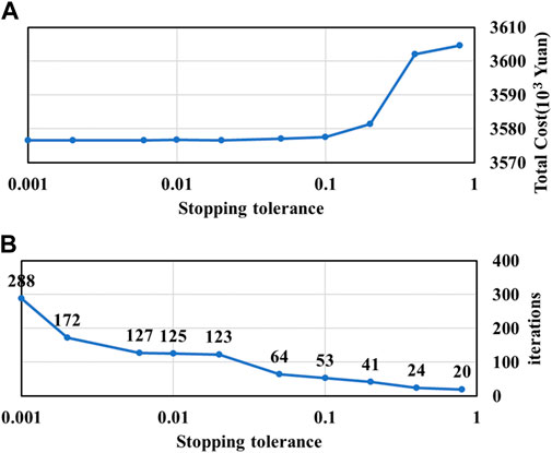
FIGURE 11. The results of convergence analysis on stopping tolerance. The impact of stopping tolerance on the total cost and the required iteration number are shown in (A,B), respectively.

The maximum allowed iterations (K) is another parameter that influences the convergence value. In a matter of fact, this parameter acts as a stopping value to ensure that the iteration is always terminated. When the number of iterations reaches K, the value of the last iteration is assigned as the result. In Figure 12, the impact of the maximum allowed iterations on the total cost of energy supply is plotted for different values of ${\epsilon }_r$. As shown in Figure 12, a lower K leads to a higher total cost, and when K is large enough, the impact on the cost is negligible because the algorithm converges before the maximum allowed iterations are reached. Therefore, there is a trade-off in parameter selection in terms of enhancing the scalability of the model and improving the optimization capability of the algorithm.

FIGURE 12

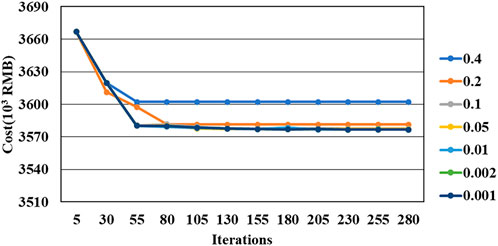
FIGURE 12. Impact of the maximum allowed iterations at different stopping tolerances on the energy supply cost.

5.6 Strengths and limitations

The proposed framework is suitable for a high-level evaluation of the long-term overall benefits considering the independent strategy of users and subsystems of IES. In the overall optimization of the multi-area IES, the behavior strategies of users and subsystems can be effectively analyzed by adopting proposed demand response and distributed optimization models. Meanwhile, in the operation optimization, the long-term overall objectives such as annual total costs and annual carbon emissions can be considered by the proposed multi-objective optimization method. Moreover, in energy trading, fairness between the users and subsystems with conflicting interests can be ensured by using the proposed profit allocation method. However, this framework may not be suitable for the operation optimization across multiple consecutive days, since the discrete typical day-based optimization is adopted to address the model complexity. The time series of consecutive days is missing in the typical day-based method. To apply this framework in operation optimization across days, the objectives such as annual total costs and annual carbon emissions need further study to enable dynamic division across seasons and multiple consecutive days.

6 Conclusion

To address the challenges of the insufficient operational independence of subsystems and unclear demand response strategies of users and unclear profit allocation in the multi-area optimization of IES, the present study proposed a holistic approach that includes user demand response as well as distributed optimization of the multi-area IES. In this study, different participants such as users and subsystems of IES are modeled as rational agents with independent optimization objectives. The multi-objective decision-making of the centralized planning approach is adopted. And fair and reasonable pricing and profit allocation method is established for the supply-demand matching and energy trading between agents with conflicting interests. The main conclusions are summarized as follows.

1) The behavior strategies of users and subsystems in the optimization process can be effectively analyzed by treating these participants as rational agents. Meanwhile, by using a distributed algorithm, the overall objective is ensured to be optimized while the subsystem is optimized.

2) The operation of subsystems is effectively regulated to meet long-term benefits by coupling long-term objectives into distributed operation optimization. Considering long-term objectives, the carbon emissions of the system operation are reduced by 9.43% compared to the case without the long-term objectives.

3) Increasing overall benefits and ensuring fairness can be achieved by using the proposed demand response and profit allocation methods. Considering profit allocation, users are more likely to purchase energy from IES than to adopt an aggressive response strategy, purchase energy from the grid or use their own supply equipment. In the case study, the energy cost of different users can decrease by 13%–17% compared to the baseline.

In summary, this study provides a holistic framework for the design and operation, supply-demand coordination, and transaction pricing of multi-area IES involving long-term planning and construction with multiple interests. The next step of the research will be focused on the combination of long- and short-term operation optimization objectives to improve the guidance for short-term operation optimization. In addition, the analysis will focus on unstable low-carbon technologies such as PV and wind power.

Data availability statement

The raw data supporting the conclusion of this article will be made available by the authors, without undue reservation.

Author contributions

XB: Conceptualization, Methodology, Software, Writing—Original Draft. LL: Validation, Writing—Review and Editing. JJ: Investigation, Writing—Review and Editing. XZ: Investigation, Writing—Review and Editing. YTZ: Validation, Writing—Review and Editing. JL: Validation, Investigation, Writing—Review and Editing. YH: Resources, Visualization. NW: Formal analysis, Resources. SX: Investigation, Data Curation, Writing—Review and Editing. YRZ: Writing—Review and Editing, Supervision, Funding acquisition.

Funding

The authors are grateful for the support from the Distinguished Young Scholars Fund of Fujian Province with Grant No. 2021J06006. The work is also supported by the National Natural Science Foundation of China under Grant No. 51876181 and the Xiamen Youth Innovation Fund with Grant No. 3502Z20206034.

Conflict of interest

The authors LL, JJ, and XZ were employed by the company Shanghai Urban Power Supply Branch, State Grid Shanghai Municipal Electric Power Company.

The remaining authors declare that the research was conducted in the absence of any commercial or financial relationships that could be construed as a potential conflict of interest.

The reviewer RJ declared a shared affiliation with the author(s) to the handling editor at the time of review.

Publisher’s note

All claims expressed in this article are solely those of the authors and do not necessarily represent those of their affiliated organizations, or those of the publisher, the editors and the reviewers. Any product that may be evaluated in this article, or claim that may be made by its manufacturer, is not guaranteed or endorsed by the publisher.

Supplementary material

The Supplementary Material for this article can be found online at: https://www.frontiersin.org/articles/10.3389/fenrg.2022.975214/full#supplementary-material

References

Arora, P., Deepali, D., and Varshney, S. (2016). Analysis of K-means and K-medoids algorithm for big data. Procedia Comput. Sci. 78, 507–512. doi:10.1016/j.procs.2016.02.095

CrossRef Full Text | Google Scholar

Bard, J. F. (2013). Practical bilevel optimization: Algorithms and applications. Berlin, Germany: Springer Science & Business Media.

Google Scholar

Berjawi, A. E. H., Walker, S. L., Patsios, C., and Hosseini, S. H. R. (2021). An evaluation framework for future integrated energy systems: A whole energy systems approach. Renew. Sustain. Energy Rev. 145, 111163. doi:10.1016/j.rser.2021.111163

CrossRef Full Text | Google Scholar

Boyd, S., Parikh, N., Chu, E., Peleato, B., and Eckstein, J. (2011). Distributed optimization and statistical learning via the alternating direction method of multipliers. FNT. Mach. Learn. 3 (1), 1–122. doi:10.1561/2200000016

CrossRef Full Text | Google Scholar

Brooke, A., Kendrick, D., Meeraus, A., Raman, R., and Rosenthal, R. J. W. (1998). Gams: A user’s guide. GAMS Development Corporation.

Google Scholar

Building Energy Research Center of Tsinghua University (2010). Annual report on China building energy efficiency. Beijing: China Building Industry Press.

Google Scholar

Chen, H., Zhang, Y., Zhang, R., Lin, C., Jiang, T., and Li, X. (2021). Privacy-preserving distributed optimal scheduling of regional integrated energy system considering different heating modes of buildings. Energy Convers. Manag. 237, 114096. doi:10.1016/j.enconman.2021.114096

CrossRef Full Text | Google Scholar

China Association of Building Energy Efficiency (2022). China building energy consumption research report [online]. Available at: https://www.efchina.org/Attachments/Report/report-20170710-1/report-20170710-1 (Accessed 01 23, 2022).

Google Scholar

Collins, S., Deane, J. P., Poncelet, K., Panos, E., Pietzcker, R. C., Delarue, E., et al. (2017). Integrating short term variations of the power system into integrated energy system models: A methodological review. Renew. Sustain. Energy Rev. 76, 839–856. doi:10.1016/j.rser.2017.03.090

CrossRef Full Text | Google Scholar

CPLEX (2019). IBM ILOG CPLEX optimization studio V12. 9.0 documentation [online]. Available at: https://www.ibm.com/docs/en/icos/12.9.0?topic=v1290-introducing-ilog-cplex-optimization-studio (Accessed 02 2022, 03).

Google Scholar

Dal Cin, E., Carraro, G., Volpato, G., Lazzaretto, A., and Danieli, P. (2022). A multi-criteria approach to optimize the design-operation of Energy Communities considering economic-environmental objectives and demand side management. Energy Convers. Manag. 263, 115677. doi:10.1016/j.enconman.2022.115677

CrossRef Full Text | Google Scholar

EnergyPlus (2022). Weather data | EnergyPlus [online]. Available at: https://energyplus.net/weather (Accessed 03 2022, 05).

Google Scholar

Environmental Change Institute & Oxford Institute for Energy Studies, and University of Oxford (2015). Assessment of demand response market potential and benefits in Shanghai [online]. Available at: http://www.nrdc.cn/Public/uploads/2016-12-03/5842cc27b4207.pdf (Accessed 04 2022, 02).

Google Scholar

ETH Zurich (2022). City energy Analyst [online]. Available at: https://cityenergyanalyst.com/try-cea (Accessed 05 2022, 13).

Google Scholar

Fonseca, J. A. (2016). Energy efficiency strategies in urban communities: Modeling, analysis and assessment. Zürich, Switzerland: ETH Zurich.

Google Scholar

Fonseca, J. A., and Schlueter, A. (2015). Integrated model for characterization of spatiotemporal building energy consumption patterns in neighborhoods and city districts. Appl. Energy 142, 247–265. doi:10.1016/j.apenergy.2014.12.068

CrossRef Full Text | Google Scholar

Gan, W., Yan, M., Yao, W., Guo, J., Ai, X., Fang, J., et al. (2021). Decentralized computation method for robust operation of multi-area joint regional-district integrated energy systems with uncertain wind power. Appl. Energy 298, 117280. doi:10.1016/j.apenergy.2021.117280

CrossRef Full Text | Google Scholar

Gao, X., Knueven, B., Siirola, J. D., Miller, D. C., and Dowling, A. W. (2022). Multiscale simulation of integrated energy system and electricity market interactions. Appl. Energy 316, 119017. doi:10.1016/j.apenergy.2022.119017

CrossRef Full Text | Google Scholar

Hart, W. E., Laird, C. D., Watson, J. P., Woodruff, D. L., Hackebeil, G. A., Nicholson, B. L., et al. (2017). Pyomo-optimization modeling in python. Berlin, Germany: Springer.

Google Scholar

Huang, T., Sun, Y., Jiao, M., Liu, Z., and Hao, J. (2022). Bilateral energy-trading model with hierarchical personalized pricing in a prosumer community. Int. J. Electr. Power & Energy Syst. 141, 108179. doi:10.1016/j.ijepes.2022.108179

CrossRef Full Text | Google Scholar

Jing, R., Wang, J., Shah, N., and Guo, M. (2021). Emerging supply chain of utilising electrical vehicle retired batteries in distributed energy systems. Adv. Appl. Energy 1, 100002. doi:10.1016/j.adapen.2020.100002

CrossRef Full Text | Google Scholar

Jing, R., Wang, M., Wang, W., Brandon, N., Li, N., Chen, J., et al. (2017). Economic and environmental multi-optimal design and dispatch of solid oxide fuel cell based CCHP system. Energy Convers. Manag. 154, 365–379. doi:10.1016/j.enconman.2017.11.035

CrossRef Full Text | Google Scholar

Jing, R., Wang, M., Zhang, Z., Liu, J., Liang, H., Meng, C., et al. (2019). Comparative study of posteriori decision-making methods when designing building integrated energy systems with multi-objectives. Energy Build. 194, 123–139. doi:10.1016/j.enbuild.2019.04.023

CrossRef Full Text | Google Scholar

Jing, R., Zhu, X., Zhu, Z., Wang, W., Meng, C., Shah, N., et al. (2018). A multi-objective optimization and multi-criteria evaluation integrated framework for distributed energy system optimal planning. Energy Convers. Manag. 166, 445–462. doi:10.1016/j.enconman.2018.04.054

CrossRef Full Text | Google Scholar

Johari, F., Peronato, G., Sadeghian, P., Zhao, X., and Widén, J. (2020). Urban building energy modeling: State of the art and future prospects. Renew. Sustain. Energy Rev. 128, 109902. doi:10.1016/j.rser.2020.109902

CrossRef Full Text | Google Scholar

Kazemi, M., and Zareipour, H. (2018). Long-term scheduling of battery storage systems in energy and regulation markets considering battery’s lifespan. IEEE Trans. Smart Grid 9 (6), 6840–6849. doi:10.1109/TSG.2017.2724919

CrossRef Full Text | Google Scholar

Keshavarzzadeh, A. H., and Ahmadi, P. (2019). Multi-objective techno-economic optimization of a solar based integrated energy system using various optimization methods. Energy Convers. Manag. 196, 196–210. doi:10.1016/j.enconman.2019.05.061

CrossRef Full Text | Google Scholar

Khorasany, M., Razzaghi, R., and Shokri Gazafroudi, A. (2021). Two-stage mechanism design for energy trading of strategic agents in energy communities. Appl. Energy 295, 117036. doi:10.1016/j.apenergy.2021.117036

CrossRef Full Text | Google Scholar

Lai, C. S., and Locatelli, G. (2021). Valuing the option to prototype: A case study with generation integrated energy storage. Energy 217, 119290. doi:10.1016/j.energy.2020.119290

CrossRef Full Text | Google Scholar

Li, L., Cao, X., and Wang, P. (2021a). Optimal coordination strategy for multiple distributed energy systems considering supply, demand, and price uncertainties. Energy 227, 120460. doi:10.1016/j.energy.2021.120460

CrossRef Full Text | Google Scholar

Li, M., Mu, H., Li, N., and Ma, B. (2016). Optimal design and operation strategy for integrated evaluation of CCHP (combined cooling heating and power) system. Energy 99, 202–220. doi:10.1016/j.energy.2016.01.060

CrossRef Full Text | Google Scholar

Li, W., Wang, S., and Koo, C. (2021b). A real-time optimal control strategy for multi-zone VAV air-conditioning systems adopting a multi-agent based distributed optimization method. Appl. Energy 287, 116605. doi:10.1016/j.apenergy.2021.116605

CrossRef Full Text | Google Scholar

Lin, J., Zhong, X., Wang, J., Huang, Y., Bai, X., Wang, X., et al. (2021). Relative optimization potential: A novel perspective to address trade-off challenges in urban energy system planning. Appl. Energy 304, 117741. doi:10.1016/j.apenergy.2021.117741

CrossRef Full Text | Google Scholar

Lyu, C., Jia, Y., and Xu, Z. (2021). Fully decentralized peer-to-peer energy sharing framework for smart buildings with local battery system and aggregated electric vehicles. Appl. Energy 299, 117243. doi:10.1016/j.apenergy.2021.117243

CrossRef Full Text | Google Scholar

Mansouri, S. A., Ahmarinejad, A., Sheidaei, F., Javadi, M. S., Rezaee Jordehi, A., Esmaeel Nezhad, A., et al. (2022). A multi-stage joint planning and operation model for energy hubs considering integrated demand response programs. Int. J. Electr. Power & Energy Syst. 140, 108103. doi:10.1016/j.ijepes.2022.108103

CrossRef Full Text | Google Scholar

Mork, M., Xhonneux, A., and Müller, D. (2022). Nonlinear distributed model predictive control for multi-zone building energy systems. Energy Build. 264, 112066. doi:10.1016/j.enbuild.2022.112066

CrossRef Full Text | Google Scholar

Nash, J. F. (1950). Equilibrium points in n -person games. Proc. Natl. Acad. Sci. U. S. A. 36 (1), 48–49. doi:10.1073/pnas.36.1.48

PubMed Abstract | CrossRef Full Text | Google Scholar

Niu, J., Tian, Z., Zhu, J., and Yue, L. (2020). Implementation of a price-driven demand response in a distributed energy system with multi-energy flexibility measures. Energy Convers. Manag. 208, 112575. doi:10.1016/j.enconman.2020.112575

CrossRef Full Text | Google Scholar

Stennikov, V., Barakhtenko, E., Mayorov, G., Sokolov, D., and Zhou, B. (2022). Coordinated management of centralized and distributed generation in an integrated energy system using a multi-agent approach. Appl. Energy 309, 118487. doi:10.1016/j.apenergy.2021.118487

CrossRef Full Text | Google Scholar

Umer, K., Huang, Q., Khorasany, M., Afzal, M., and Amin, W. (2021). A novel communication efficient peer-to-peer energy trading scheme for enhanced privacy in microgrids. Appl. Energy 296, 117075. doi:10.1016/j.apenergy.2021.117075

CrossRef Full Text | Google Scholar

Wang, H., and Huang, J. (2018). Incentivizing energy trading for interconnected microgrids. IEEE Trans. Smart Grid 9 (4), 2647–2657. doi:10.1109/TSG.2016.2614988

CrossRef Full Text | Google Scholar

Wang, H., Zhang, C., Li, K., Liu, S., Li, S., and Wang, Y. (2021). Distributed coordinative transaction of a community integrated energy system based on a tri-level game model. Appl. Energy 295, 116972. doi:10.1016/j.apenergy.2021.116972

CrossRef Full Text | Google Scholar

Wang, M., Yu, H., Jing, R., Liu, H., Chen, P., and Li, C. (2020). Combined multi-objective optimization and robustness analysis framework for building integrated energy system under uncertainty. Energy Convers. Manag. 208, 112589. doi:10.1016/j.enconman.2020.112589

CrossRef Full Text | Google Scholar

Wang, Y., Wang, J., Liu, Z., Liu, Y., and Tan, Z. (2022). Multi-objective synergy planning for regional integrated energy stations and networks considering energy interaction and equipment selection. Energy Convers. Manag. 251, 114986. doi:10.1016/j.enconman.2021.114986

CrossRef Full Text | Google Scholar

Wen, Y., Qu, X., Li, W., Liu, X., and Ye, X. (2018). Synergistic operation of electricity and natural gas networks via ADMM. IEEE Trans. Smart Grid 9, 4555–4565. doi:10.1109/tsg.2017.2663380

CrossRef Full Text | Google Scholar

Xi, Y., Fang, J., Chen, Z., Zeng, Q., and Lund, H. (2021). Optimal coordination of flexible resources in the gas-heat-electricity integrated energy system. Energy 223, 119729. doi:10.1016/j.energy.2020.119729

CrossRef Full Text | Google Scholar

Xiang, Y., Cai, H., Gu, C., and Shen, X. (2020). Cost-benefit analysis of integrated energy system planning considering demand response. Energy 192, 116632. doi:10.1016/j.energy.2019.116632

CrossRef Full Text | Google Scholar

Zhang, D., Evangelisti, S., Lettieri, P., and Papageorgiou, L. G. (2015). Optimal design of CHP-based microgrids: Multiobjective optimisation and life cycle assessment. Energy 85, 181–193. doi:10.1016/j.energy.2015.03.036

CrossRef Full Text | Google Scholar

Zhang, Y., Campana, P. E., Lundblad, A., Zheng, W., and Yan, J. (2019). Planning and operation of an integrated energy system in a Swedish building. Energy Convers. Manag. 199, 111920. doi:10.1016/j.enconman.2019.111920

CrossRef Full Text | Google Scholar

Zheng, L., Zhou, B., Cao, Y., Wing Or, S., Li, Y., and Wing Chan, K. (2022). Hierarchical distributed multi-energy demand response for coordinated operation of building clusters. Appl. Energy 308, 118362. doi:10.1016/j.apenergy.2021.118362

CrossRef Full Text | Google Scholar

Zheng, W., Wu, W., Zhang, B., Sun, H., and Liu, Y. (2016). A fully distributed reactive power optimization and control method for active distribution networks. IEEE Trans. Smart Grid 7 (2), 1021–1033. doi:10.1109/TSG.2015.2396493

CrossRef Full Text | Google Scholar

Zhou, Y., Wu, J., Song, G., and Long, C. (2020). Framework design and optimal bidding strategy for ancillary service provision from a peer-to-peer energy trading community. Appl. Energy 278, 115671. doi:10.1016/j.apenergy.2020.115671

CrossRef Full Text | Google Scholar

Nomenclature

Abbreviations

IES integrated energy system

ADMM alternating direction method of multipliers

LA load aggregator

CHP combined heat and power

HP heat pump

AC absorption chiller

EC electric chiller

PV photovoltaic

WT wind turbine

BES battery energy storage

TST thermal storage tank

MILP mixed integer linear programming

CAPEX capital expenditure

FC fuel cost

MC maintenance cost

CRF capital recovery factor

ATC annual total cost

ACE annual carbon emission

Symbols

Obj objective function

C cost

E energy demand for users and energy supply for suppliers

Q thermal energy

prob probability of each typical day

Greek symbols

$\lambda$ Lagrangian operator

$\rho$ penalty factor

$\epsilon$ stopping tolerance

$\eta$ efficiency

$\theta$ fitting parameters

$\sigma$ heat-power ratio of CHP

$\chi$ on/off status

Subscripts/superscripts

b boiler

el electricity

he heating

co cooling

i user

n supplier

s typical day

h hour

k iteration

emi carbon emission

L lower bound