Light intensity optimization of optical fiber stress sensor based on SSA-LSTM model

In order to further improve the measurement range and accuracy of optical fiber stress sensor based on the interference between rising vortex beam and plane wave beam, a new stress demodulation model is designed. This model proposes a method to optimize the long-term and short-term memory network (LSTM) model by using sparrow search algorithm (SSA), extract the main characteristics of the influence of various variables on optical fiber stress sensor, and fit the relationship between sensor stress and beam phase difference. This method is an attempt of the deep learning model LSTM in the study of stress mediation model. There are very few related studies, and it is very necessary to fill this gap. In the experiment, the SSA-LSTM neural network is trained by using the data of stress and phase difference measured by the optical fiber stress sensor. The test results show that the mean error of SSA-LSTM neural network is less than that of LSTM neural network, which shows that the combination of SSA-LSTM model and optical fiber stress sensor can make its measurement accuracy higher, The algorithm can more effectively reduce the influence of the surrounding environment and the influence of the light source fluctuation on the measurement range and accuracy of the optical fiber sensor, and has good practical application value. It is proved that the deep learning LSTM neural network has good application value in the light intensity optimization of optical fiber stress sensor.

Introduction

Force sensor is one of the most important components in the robot control system, especially at the robot joint. When installed on the robot’s foot and wrist, it can realize the functions of robot center of gravity tendency perception and balance state monitoring, and plays an irreplaceable role in the force analysis and stability of the robot. Traditional mechanical sensors mainly include resistive sensors, capacitive sensors, etc. (Zhou et al., 2014; Yue et al., 2022), which have the characteristics of high precision and high sensitivity, and are widely used in various mechanical sensing fields. However, traditional resistive sensors and capacitive sensors are vulnerable to electromagnetic interference, corrosion, high temperature and high voltage, and can not be used normally in harsh environment (Zm et al., 2020).

Optical fiber sensor has the advantages of light weight, small volume, high sensitivity and easy reuse to form distributed measurement. It is widely used to measure physical quantities such as stress and strain in engineering projects such as bridge construction, pipeline leakage and deepwater riser (Zhao et al., 2021). Researchers have proposed various types of optical fiber stress sensors (Asriani et al., 2020; Cai et al., 2020; Guo et al., 2020; Tan et al., 2020; Zheng et al., 2020; Tang et al., 2021; Xiang, 2021), which are based on single-mode multi-mode single-mode tapered fiber Bragg grating sensors. The measurement range of the sensor is 0–960 με; A Fabry Perot based strain sensor (He et al., 2020). The cavity is formed by splicing a new advanced silicon tube between two standard single-mode fibers. The maximum strain range measured by the sensor is 2500 με。 However, these sensors usually use ordinary Gaussian light source, and due to the limitation of the structure itself, they can not measure large strain, or the measurement results have errors.

In recent years, with the continuous development of vortex rotation, some scholars have proposed an optical fiber sensor based on vortex rotation. According to the spiral and fork characteristics of the interference pattern between vortex and Gaussian light, researchers have proposed several different types of interference optical fiber sensors. A new strain sensing method based on the interference of vortex light and Gaussian spherical wave (Ning et al., 2020). The rotation angle of spiral image caused by strain is recognized by digital image processing technology. In theory, high-resolution strain measurement can be realized, but no experimental research has been carried out. An optical fiber stress sensor based on the interference between vortex beam and plane wave beam extracts two main features of interference pattern set by principal component analysis (PCA) (Lv et al., 2018), and realizes the demodulation process according to the variation law of interference pattern correlation coefficient group corresponding to different phase difference, but the demodulation process is complex and the stress measurement range is small.

In this paper, the optical power output of optical fiber stress sensor depends on many environmental factors, such as ambient light change, vibration noise and light source fluctuation. The measurement of optical fiber stress sensor depends on the stress phase difference relationship of light and the change value of power. The output optical power value will be affected by the fluctuation of light source and the coupling between light source and optical fiber, resulting in measurement error. In view of the nonlinear impact of the above problems, the hardware and software can be optimized, and the hardware can be replaced with a new structure. Although the above problems can be solved to a certain extent, it will lead to the increase of cost and circuit complexity, and the electronic devices themselves will also produce new interference, which will affect the range and accuracy of the whole optical fiber stress sensor measurement system.

Therefore, it is necessary to introduce the algorithm to optimize the experimental data in order to improve the measurement accuracy of the optical fiber stress sensor system. Based on the short-term and long-term memory network method optimized by sparrow search algorithm, SSA-LSTM neural network is proposed to improve the measurement accuracy. Because the LSTM network is a nonlinear optimization, the weights and thresholds are generated randomly, which will cause the structure to be accidental and locally optimal (Jiang et al., 2021). The search of SSA (sparrow search algorithm) algorithm is based on the optimal location and the historical optimal location of all discoverers in the population, which can quickly achieve the goal of global optimization. This feature can be used to optimize the weight and threshold of LSTM neural network and avoid falling into the situation of partial optimization in solvable space (Yao et al., 2022). This paper introduces the composition of optical fiber stress sensor measurement system, the principle and method of experiment and the principle of sparrow search algorithm optimizing LSTM neural network, and compares the experimental data after light intensity optimization of SSA-LSTM neural network with the experimental data of LSTM neural network without optimized weight threshold, which provides a certain reference value for improving the measurement range and precision optimization of optical fiber stress sensor.

Methodology

Fiber optic stress sensing system structure

The design of stress sensing system based on the interference between vortex beam and plane wave beam is shown in Figure 1. The light source is a 632.8 nm He Ne laser. After passing through a 1:1 beam splitter, the collimated laser is divided into a reference light path and a sensing light path: the reference light path is coupled into a 3 m long single-mode fiber through a lens with a focal length of 240 mm, emitted through a fiber collimator (74UV-FC), and then the first-order vortex light is obtained through a polarizer, a quarter wave plate and a vortex wave plate (VR1-633); The sensing optical path is coupled into a 3 m long single-mode optical fiber through a lens with a focal length of 240 mm. The single-mode optical fiber is fixed on the tensile test bench. After being emitted by the optical fiber collimator (74UV-FC), the plane wave beam is obtained through the polarizer. Finally, the reference light interferes with the sensing light beam mirror, and the charge coupled element (CCD) collects the interference pattern.

FIGURE 1

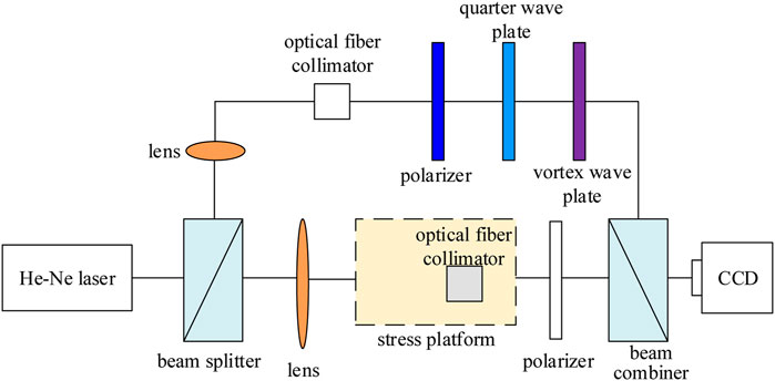
FIGURE 1. Fiber optic stress sensing system structure.

Principle of light interference in sensing system

Vortex light is a special light field with helical phase wavefront. The phase distribution contains $\exp \left(il\theta \right)$ term, $\theta$ is the rotation azimuth and $l$ is the topological charge. When the vortex light propagates along the positive direction of the $Z$ axis, the complex amplitude $E_1$ of the electric field on the observation surface (Ying et al., 2021) with $Z=0$ can be expressed as:

$E_1\left(X,Y\right)=E_0\exp \left(il\theta +i\phi \right)(1)$

Where $E_0$ is the beam amplitude and $\phi$ is the additional phase difference.

When the plane wave with inclined wavefront propagates along the $Z$ axis direction, the complex amplitude $E_2$ of the electric field on the observation surface with $Z=0$ can be expressed as:

$E_2\left(X,Y\right)=E_0\exp \left(ikX\sin \alpha \right)(2)$

Where $X$ is the component of rectangular coordinate system, $k$ is the wave number, and $\alpha$ is the included angle between $k$ and the positive direction of $Z$ axis.

If two beams of light interfere on the plane of $Z=0$, according to $E=E_1+E_2$, the expression of electric field E after interference is:

$E=E_0\exp \left(il\theta +i\phi \right)+E_0\exp \left(ikX\sin \alpha \right)(3)$

According to $I=E{E}^{\ast }$, the light intensity distribution $I$ after interference is:

$I=2+2\cos \left(l\theta +\phi -kX\sin \alpha \right)(4)$

System optimization by SSA-LSTM

The SSA-LSTM model is used to extract the main characteristics of the interference wave, and the relationship between the phase difference between the two beams and the correlation coefficient of the corresponding main characteristics of the interference is fitted. According to the stress phase difference relationship, the relationship between the stress and the correlation coefficient is obtained.

LSTM neural network

LSTM makes information selectively affect the state of each time in the model by adding gate structure (Vpn et al., 2021; Delgado et al., 2020), which is mainly composed of input gate, output gate and forgetting gate. The specific formula is shown in (5–10), and the specific structure of LSTM unit is shown in Figure 2.

FIGURE 2

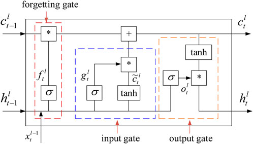
FIGURE 2. Cell structure of LSTM.

If the input is $[x_1,x_2,\mathrm{...},x_t]$ and the state of the hidden layer is $[h_1,h_2,\mathrm{...},h_t]$, the following operations are performed at time $t$:

(1) Forgetting gate operation: determine whether to forget the hidden cell state $h_t^{l-1}$ transmitted by the upper layer with a certain probability in LSTM, and control the output range between [0,1] through sigmoid function. See formula (5) for details.

$f_t^l=\sigma \left(w_f^l\cdot \left[h_{t-1}^l,x_t^{l-1}\right]+b_f^l\right)(5)$

In Eq. 5, $\sigma \left(\right)$ is the activation function, $•$ is the vector inner product, $t$ is the time, $l$ is the number of layers of LSTM neural network, $f$ is the forgetting gate, $w$ is the weight, $b$ is the bias, and $h$ is the cell output.

(2) Input gate operation: the input gate consists of two parts. Sigmoid and tanh activation functions are used to control the range of output value respectively, and the product of the two parts is used to participate in the update of cell state. See formulas (6) and (7) for details.

$g_t^l=\sigma \left(w_g^l\cdot \left[h_{t-1}^l,x_t^{l-1}\right]+b_g^l\right)(6)$

${\tilde{c}}_t^l=\tanh \left(w_c^l\cdot \left[h_{t-1}^l,x_t^{l-1}\right]+b_c^l\right)(7)$

In Eqs 6, 7, tanh ( ) is the activation function, $g$ represents the input gate, $c$ represents the cell state, and $\tilde{c}$ represents the current input unit state.

(3) Cell state update: the cell state is updated by calculating the product of the cell state at the previous time and the output of the forgetting gate and the product of the results of the two parts of the input gate, and adding the products of the two parts. See formula (8) for details.

$c_t^l=f_t^l\ast c_{t-1}^l+g_t^l\ast {\tilde{c}}_t^l(8)$

Equation 8, * represents the multiplication of the elements of the corresponding dimensions of two vectors.

(4) Output gate operation: the output gate consists of two parts. The first part is also the hidden state at the previous time and the input variable at this time as the input, and the output range is controlled by sigmoid function. The second part controls the output range by tanh activation function, and then multiplies the output result of the first part to update the hidden layer state. The specific formulas are as follows (9) and (10).

$o_t^l=\sigma \left(w_o^l\cdot \left[h_{t-1}^l,x_t^{l-1}\right]+b_o^l\right)(9)$

$h_t^l=o_t^l\cdot \tanh \left(c_t^l\right)(10)$

$o$ in Eqs 9, 10 represents the output gate.

SSA optimization algorithm

Sparrow search algorithm (SSA) (Jia et al., 2022; Qi et al., 2021; Wc et al., 2021) is a new intelligent optimization algorithm based on sparrows’ foraging behavior and anti predation behavior. The algorithm can optimize several super parameters of LSTM at the same time, and has strong optimization ability and convergence speed. The basic theory of SSA optimization algorithm is as follows:

When using SSA algorithm to optimize the super parameters of LSTM model, $n$ sparrows form a population to search for food. The population is expressed as follows:

$X=\left[\begin{array}{cccc}{x}_{\mathrm{1,1}}& x_{\mathrm{1,2}}& \mathrm{...}& x_{1,d}\\ x_{\mathrm{2,1}}& x_{\mathrm{2,2}}& \mathrm{...}& x_{2,d}\\ \mathrm{...}& \mathrm{...}& \mathrm{...}& \mathrm{...}\\ x_{n,1}& x_{n,2}& \mathrm{...}& x_{n,d}\end{array}\right](11)$

Where, $d$ represents the dimension of the problem to be optimized. Therefore, the sparrow fitness value is expressed as follows:

$F_X=\left[\begin{array}{c}f\left(\left[\begin{array}{cccc}{x}_{\mathrm{1,1}}& x_{\mathrm{1,2}}& \mathrm{...}& x_{1,d}\end{array}\right]\right)\\ f\left(\left[\begin{array}{cccc}{x}_{\mathrm{2,1}}& x_{\mathrm{2,2}}& \mathrm{...}& x_{2,d}\end{array}\right]\right)\\ \mathrm{...}\\ f\left(\left[\begin{array}{cccc}{x}_{n,1}& x_{n,2}& \mathrm{...}& x_{n,d}\end{array}\right]\right)\end{array}\right](12)$

Where $f$ is the fitness value.

Since the discoverer provides foraging directions for all participants, once the existence of predators is found, the individual starts to sound an alarm. If the alarm value is greater than the safe value, the discoverer will shift the location and bring the participants into a new area for foraging. During the iteration, the location of the discoverer is updated as follows:

$X_{i,j}^{t+1}=\{\begin{array}{ccc}{X}_{i,j}^t\cdot \exp \left(-\frac{i}{\alpha \cdot T}\right)& if& R_2<ST\\ X_{i,j}^t+Q\cdot L& if& R_2\ge ST\end{array}(13)$

Where $t$ represents the current number of iterations, $T$ is the maximum number of iterations, $j=\mathrm{1,2},\mathrm{...},d$. $X_{i,j}$ represents the position information of the ith sparrow in the $j$ dimension. $R_2$ and St are the early warning value and safety value respectively. The ranges are [0,1], [0.5,1] and $\alpha$ is a random number within [0,1]. $L$ is the matrix of $1\times d$ whose internal elements are all 1. Among them, when the early warning value is less than the safety value, the sparrow can perform the search operation. When the early warning value is greater than the safety value, it indicates that predators have appeared within the search range, and all sparrows need to be transferred to a safe place to look for food immediately.

For those who join in the process of sparrow foraging, if the energy is too low, they need to fly to other places for foraging to obtain more energy. Some participants will compete for food in order to increase their energy and even monitor the discoverer. If the participants win, they will get new food. The location update is shown in the formula:

$X_{i,j}^{t+1}=\{\begin{array}{ccc}Q\cdot \exp \left(\frac{X_{worst}-X_{i,j}^t}{i^2}\right)& if& i>n/2\\ X_p^{t+1}+\left|X_{i,j}^t-X_p^{t+1}\right|\cdot A^T{\left(A{A}^T\right)}^{-1}\cdot L& if& otherwise\end{array}(14)$

Where $A$ is a $1\times d$ matrix, each element is 1 or - 1, $X_{worst}$ is the global worst position, and $X_p$ is the best position occupied by the current discoverer.

During the experiment, we assume that the number of sparrows aware of danger accounts for 10%–20%. The location of these sparrows is shown in formula (8):

$X_{i,j}^{t+1}=\{\begin{array}{ccc}{X}_{best}^t+\beta \cdot \left|X_{i,j}^t-X_{best}^t\right|& if& f_i>f_g\\ X_{i,j}^t+K\cdot \left(\left|\frac{X_{i,j}^t-X_{worst}^t}{(f_i-f_w)+\epsilon }\right|\right)& if& f_i=f_g\end{array}(15)$

$X_{best}$ and $\beta$ are the globally optimal position and step control parameters respectively, which obey the standard normal distribution. $f_i$, $f_g$ and $f_w$ are the fitness values of individual sparrow, global optimal position and worst position respectively, $K\in [-\mathrm{1,1}]$, $\epsilon$ is a very small constant, in order to avoid the occurrence of zero denominator.

In formula (8), when $f_i=f_g$, it indicates that the sparrows in the population have realized the danger and need to quickly move to other positions to avoid being preyed on, where $K$ is the moving step.

The algorithm calculates the fitness of sparrows in the population and sorts them to select the optimal value and the worst value; Then, update the location of the discoverer, entrant and aware of the dangerous sparrow. Finally, obtain the current best location. If the current location is better than the result of the previous iteration, stop the iteration. Otherwise, continue the iteration until the termination conditions are met. The process is shown in Figure 3.

FIGURE 3

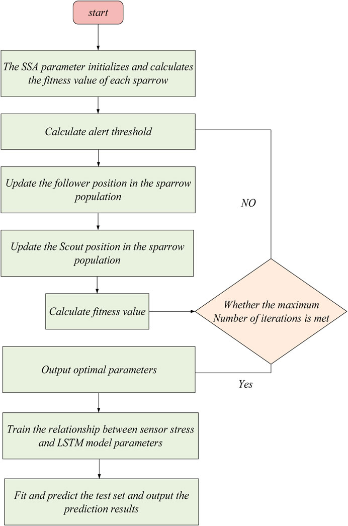
FIGURE 3. Flow chart of LSTM optimized based on SSA.

Experimental comparison and analysis

In this paper, the sensing system (Figure 1) is built to study the response characteristics of stress sensing. The optical fiber in the sensing optical path is fixed on the tension platform, and the stress is applied from 10.18 MPa to 50.88 mpa in steps of 4.07 MPa, that is, the maximum value of strain measurement is 3492 με, CCD collects interferograms corresponding to different stresses (Li et al., 2021a; Li et al., 2021b; Li 2022a; Li 2022b).

General collection and mediation methods

According to the analysis process in Section 2.1 and Figure 4 is the collected picture, this paper processes the bifurcation interferogram collected in the experiment, regards the collected interferogram as a pattern set, calculates the main features of the pattern set, obtains the correlation coefficient ${\omega }_1$ of each interferogram for the main features, and obtains the relationship between the correlation coefficient ${\omega }_1$ of the bifurcation interferogram and the stress, as shown in Figure 5. It can be seen that there is a periodic trigonometric function distribution between stress and correlation coefficient ${\omega }_1$. Through trigonometric function curve fitting, the fitting degree $R^2$ is 0.94591. In order to obtain high-quality images and improve the fitting effect, higher precision CCD equipment can be used to collect interference patterns. The mathematical expression of the demodulation model obtained by fitting is:

$y=y_0+A\sin \left(\pi \frac{x-x_c}{\omega }\right)(16)$

FIGURE 4

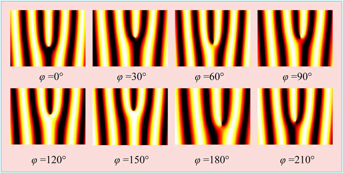
FIGURE 4. Interference patterns corresponding to different phase differences.

FIGURE 5

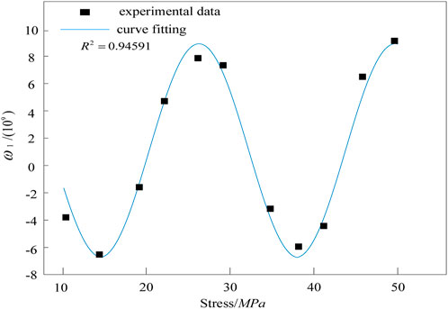
FIGURE 5. Relationship between characteristic correlation coefficient ${\omega }_1$ and stress.

Where, $y$ is the correlation coefficient of the main features of the fitted fork image, $x$ is the stress, and $y_0$, $A$, $\omega$ and $x_c$ are the known constants, $y_0\approx 0.39813$, $A\approx 7.03067$, $\omega$ and $x_c$. This document defines:

$\left(y-y_0\right)/A=\beta (17)$

$\sin \left(\pi \frac{x-x_c}{\omega }\right)=\sin \alpha (18)$

It can be obtained according to Eqs 17, 18

$\beta =\sin \alpha (19)$

According to the properties of trigonometric function, given the value of $\beta$ and the shape of $\beta -\alpha$ curve, the value of a can be expressed as:

$\{\begin{array}{c}\alpha =2k\pi +\mathrm{a}\mathrm{r}\mathrm{c}\mathrm{s}\mathrm{i}\mathrm{n}\mathit{\beta },-\frac{\pi }{2}+2k\pi \le \alpha \le \frac{\pi }{2}+2k\pi \left(\mathrm{I}\mathrm{n}\mathrm{c}\mathrm{r}\mathrm{e}\mathrm{a}\mathrm{s}\mathrm{i}\mathrm{n}\mathrm{g}\mathrm{i}\mathrm{n}\mathrm{t}\mathrm{e}\mathrm{r}\mathrm{v}\mathrm{a}\mathrm{l}\right)\\ \alpha =\left(2k+1\right)\pi -\arcsin \beta ,\frac{\pi }{2}+2k\pi <\alpha <\frac{3}{2}\pi +2k\pi \left(\mathrm{D}\mathrm{e}\mathrm{c}\mathrm{r}\mathrm{e}\mathrm{a}\mathrm{s}\mathrm{i}\mathrm{n}\mathrm{g}\mathrm{i}\mathrm{n}\mathrm{t}\mathrm{e}\mathrm{r}\mathrm{v}\mathrm{a}\mathrm{l}\right)\end{array}(20)$

Where $k$ is an integer, that is, the number of cycles from $\alpha =0$.

Judge the period and monotonic interval of $\alpha$ at any position according to Figure 4, and substitute Eq. 20 to calculate the $\alpha$ value of each point. It is concluded that there is a linear relationship between $\alpha$ and stress, as shown in Figure 6. The fitting curve can be expressed as:

$\alpha =7.21344+0.25694x(21)$

FIGURE 6

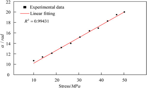
FIGURE 6. Relationship between $\alpha$ and different stresses.

The fitting results show that the phase adjustment method can achieve the sensitivity of stress measurement of 0.257 rad/MPa.

Fitting method based on SSA-LSTM

The method based on SSA-LSTM takes the relationship between ${\omega }_1$, $\alpha$ and stress as training data, and fits a more suitable corresponding relationship through the training of neural network. Because the LSTM model is suitable for fitting the relationship between nonlinear quantities, this method is different from the method in Section 3.1. SSA-LSTM does not need to fit any relevant equations or mathematical expressions. Instead, it tests the values between the stress of multiple groups of data and relevant variables, and takes these values as the training data of the model. Through training, the corresponding values can be obtained through SSA-LSTM by inputting the measured data without mathematical calculation.

For example, taking the data in Section 3.1 as the test, the fitting curve of the relationship between the characteristic correlation coefficient ${\omega }_1$ and stress is finally obtained, as shown in Figure 7. It can be seen that there is a periodic trigonometric function distribution between stress and correlation coefficient ${\omega }_1$. Through trigonometric function curve fitting, the fitting degree $R^2$ is 0.98591, which is higher than the fitting degree 0.94591 of the formula calculation method used in 3.1. Similarly, for the relationship between $\alpha$ and stress, the fitting degree is 0.99893, which is more accurate than the method without LSTM neural network. As shown in Figure 8, the fitting curve is expressed as:

$\alpha =7.31361+0.28634x(22)$

FIGURE 7

FIGURE 7. Relationship between characteristic correlation coefficient ${\omega }_1$ and stress.

FIGURE 8

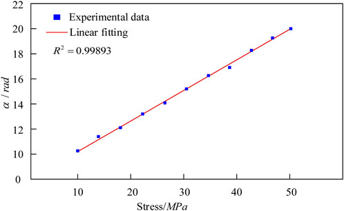
FIGURE 8. Relationship between $\alpha$ and different stresses.

The fitting results show that using SSA-LSTM method, the sensitivity of stress measurement can be 0.286 rad/MPa, which is greater than the original 0.257, so the performance is better.

Conclusion

In this paper, an optical fiber stress sensing system is designed, and a new stress demodulation model is proposed. The feasibility of realizing large range monitoring by the sensor is verified by simulation and experiment. In the experiment, an interferometric sensing system based on vortex rotation light is built, and the fork interferograms corresponding to different stresses are collected. The main features of the fork interferogram are extracted by SSA-LSTM method. Through model regression analysis, the periodic triangular function distribution of the correlation coefficient between the stress and the image is obtained; Through further training and fitting of LSTM model, the linear relationship related to stress is obtained. The experimental results show that the sensitivity of the sensing system is 0.286 rad/MPa and the maximum measurement range is 3492 με. In this study, the performance of deep learning model has been greatly improved by applying it to the related research of fiber optic stress sensor. In the future, deep learning will be combined with more studies and be more fully applied.

Data availability statement

The raw data supporting the conclusions of this article will be made available by the authors, without undue reservation.

Author contributions

DY and XQ conceived the idea and designed the experiments. XW and XQ led the experiments and contributed to data analysis and interpretation. DY and XW wrote the paper. All authors read and approved the final manuscript.

Funding

1 The National Natural Science Foundation of China (Nos.61735041, 61927812).

2 Scientific Research Program Funded by Shaanxi Provincial Education Department of China (No.08JS093).

Conflict of interest

The authors declare that the research was conducted in the absence of any commercial or financial relationships that could be construed as a potential conflict of interest.

Publisher’s note

All claims expressed in this article are solely those of the authors and do not necessarily represent those of their affiliated organizations, or those of the publisher, the editors and the reviewers. Any product that may be evaluated in this article, or claim that may be made by its manufacturer, is not guaranteed or endorsed by the publisher.

References

Asriani, F., Winasis, , and Pamudji, G. (2020). Sensitivity of optical fiber sensors to deflection of reinforced concrete beam. IOP Conf. Ser. Mat. Sci. Eng. 982, 012025. doi:10.1088/1757-899x/982/1/012025

CrossRef Full Text | Google Scholar

Cai, Y., Li, M., Wang, M., Li, J., Zhang, Y., and Zhao, Y. (2020). Optical fiber sensors for metal ions detection based on novel fluorescent materials. Front. Phys. 8, 598209. doi:10.3389/fphy.2020.598209

CrossRef Full Text | Google Scholar

Delgado, I., and Fahim, M. (2020). Wind turbine data analysis and LSTM-based prediction in SCADA system. Energies 14, 125. doi:10.3390/EN14010125

CrossRef Full Text | Google Scholar

Guo, J., Geng, T., Yan, H., Du, L., Zhang, Z., and Sun, C. (2020). Implementation of a load sensitizing bridge spherical bearing based on low-coherent fiber-optic sensors combined with neural network algorithms. Sensors 21 (1), 37. doi:10.3390/s21010037

CrossRef Full Text | Google Scholar

He, X., Ran, Z., Xiao, Y., Xu, T., Shen, F., Ding, Z., et al. (2020). Three-dimensional force sensors based on all-fiber Fabry-Perot strain sensors. Opt. Commun. 490, 126694. doi:10.1016/j.optcom.2020.126694

CrossRef Full Text | Google Scholar

Jia, J., Yuan, S., Shi, Y., Wen, J., Pang, X., and Zeng, J. (2022). Improved sparrow search algorithm optimization deep extreme learning machine for lithium-ion battery state-of-health prediction. iScience 25 (4), 103988. doi:10.1016/j.isci.2022.103988

PubMed Abstract | CrossRef Full Text | Google Scholar

Jiang, Z., Hu, W., and Qin, H. (2021). WSN node localization based on improved sparrow search algorithm optimization. Int. Conf. Sensors Instrum. 2021, 11887. doi:10.1117/12.2602966

CrossRef Full Text | Google Scholar

Li, H. (2022b). SCADA data based wind power interval prediction using LUBE-based deep residual networks. Front. Energy Res. 10, 920837. doi:10.3389/fenrg.2022.920837

CrossRef Full Text | Google Scholar

Li, H. (2022a). Short-term wind power prediction via spatial temporal analysis and deep residual networks. Front. Energy Res. 10, 920407. doi:10.3389/fenrg.2022.920407

CrossRef Full Text | Google Scholar

Li, H., Deng, J., Feng, P., Pu, C., Arachchige, D. D., and Cheng, Q. (2021b). Short-term nacelle orientation forecasting using bilinear transformation and ICEEMDAN framework. Front. Energy Res. 697, 780928. doi:10.3389/fenrg.2021.780928

CrossRef Full Text | Google Scholar

Li, H., Deng, J., Yuan, S., Feng, P., and Arachchige, D. D. (2021a). Monitoring and identifying wind turbine generator bearing faults using deep belief network and EWMA control charts. Front. Energy Res. 9, 770. doi:10.3389/fenrg.2021.799039

CrossRef Full Text | Google Scholar

Lv, R., Qiu, L., Hu, H., Meng, L., and Zhang, Y. (2018). The phase interrogation method for optical fiber sensor by analyzing the fork interference pattern. Appl. Phys. B 124 (2), 32. doi:10.1007/s00340-018-6901-5

CrossRef Full Text | Google Scholar

Ning, X., Duan, P., and Zhang, S. (2020). Real-time 3D face alignment using an encoder-decoder network with an efficient deconvolution layer. IEEE Signal Process. Lett. 27, 1944–1948. doi:10.1109/LSP.2020.3032277

CrossRef Full Text | Google Scholar

Qi, S., Ning, X., Yang, G., Zhang, L., Li, W., Cai, W., et al. (2021). Review of multi-view 3D object recognition methods based on deep learning. Displays 69 (1), 102053. doi:10.1016/j.displa.2021.102053

CrossRef Full Text | Google Scholar

Tan, X., and Bao, Y. (2020). Measuring crack width using a distributed fiber optic sensor based on optical frequency domain reflectometry. Measurement 172, 108945. doi:10.1016/j.measurement.2020.108945

CrossRef Full Text | Google Scholar

Tang, F., Zhou, G., Li, H., and Verstrynge, E. (2021). A review on fiber optic sensors for rebar corrosion monitoring in RC structures. Constr. Build. Mater. 313, 125578. doi:10.1016/j.conbuildmat.2021.125578

CrossRef Full Text | Google Scholar

Vpn, A., Hao, L., At, A., Chao, H., and Atzc, D. (2021). Ensembles of probabilistic LSTM predictors and correctors for bearing prognostics using industrial standards. Neurocomputing 491, 575–596. doi:10.1016/j.neucom.2021.12.035

CrossRef Full Text | Google Scholar

Wc, A., Dong, L., Xin, N., Chen, W., and Gx, D. (2021). Voxel-based three-view hybrid parallel network for 3d object classification. Displays 69, 102076. doi:10.1016/j.displa.2021.102076

CrossRef Full Text | Google Scholar

Xiang, P., and Wang, H. P. (2021). Optical fiber sensors for monitoring railway infrastructures: A review towards smart concept. Symmetry 13, 2251. doi:10.3390/sym13122251

CrossRef Full Text | Google Scholar

Yao, Ji., Wu, W., and Li, S. (2022). Anomaly detection model of mooring system based on LSTM PCA method. Ocean. Eng. 254, 111350. doi:10.1016/j.oceaneng.2022.111350

CrossRef Full Text | Google Scholar

Ying, L., Nan, Z., Ping, W., Kiang, C., Pang, L., Chang, Z., et al. (2021). Adaptive weights learning in cnn feature fusion for crime scene investigation image classification. Connect. Sci. 33 (3), 719–734. doi:10.1080/09540091.2021.1875987

CrossRef Full Text | Google Scholar

Yue, Q., Xiao, S., Li, Z., Yang, J., Chen, B., Feng, J., et al. (2022). Ultra-sensitive pressure sensors based on large alveolar deep tooth electrode structures with greatly stretchable oriented fiber membrane. Chem. Eng. J. 443, 136370. doi:10.1016/j.cej.2022.136370

CrossRef Full Text | Google Scholar

Zhao, M., Zhou, X., and Chen, Y. (2021). A highly sensitive and miniature optical fiber sensor for electromagnetic pulse fields. Sensors 21 (23), 8137. doi:10.3390/s21238137

PubMed Abstract | CrossRef Full Text | Google Scholar

Zheng, H., Lv, R., Zhao, Y., Tong, R., Lin, Z., Wang, X., et al. (2020). Multifunctional optical fiber sensor for simultaneous measurement of temperature and salinity. Opt. Lett. 45 (24), 6631–6634. doi:10.1364/OL.409233

PubMed Abstract | CrossRef Full Text | Google Scholar

Zhou, J., Wang, Y., Liao, C., Yin, G., Li, Z., Yang, K., et al. (2014). Intensity-modulated strain sensor based on fiber in-line mach-zehnder interferometer. IEEE Photonics Technol. Lett. 26 (5), 508–511. doi:10.1109/LPT.2013.2295826

CrossRef Full Text | Google Scholar

Zm, A., Kib, C., Gz, B., Yw, A., Ml, A., and Lei, W. (2020). Foot type classification using sensor-enabled footwear and 1D-CNN. Measurement 165, 108184. doi:10.1016/j.measurement.2020.108184

CrossRef Full Text | Google Scholar