 David H. Wood
 Mohamed M. Hammam
- 1Department of Mechanical and Manufacturing Engineering, University of Calgary, Calgary, AB, Canada
- 2Departement of Mechanical Power Engineering, Faculty of Engineering, Port Said University, Port Said, Egypt
This study analyzes actuator disc (AD) models of horizontal-axis turbines to determine optimal performance, defined as the maximum power extracted at any tip speed ratio. We use the calculus of variations to maximize rotor torque relative to the thrust without making any assumptions about the rotor loading. The torque was obtained from the angular momentum equation and the thrust from the Kutta-Joukowsky equation which depends on the circumferential velocity and tip speed ratio. The optimality requirement is that the pitch of the vorticity exiting the rotor must be constant across the wake and equal to the ratio of torque to thrust. This result generalizes the classical finding of Betz and Goldstein that optimal lightly-loaded ADs have constant pitch. Optimizing the torque in the far-wake, well downstream of the rotor, leads to the same requirement of constant pitch. This implies that the pitch of an optimal rotor is constant everywhere in the wake at all tip speed ratios. We show that it is not possible for the pitch to reach its optimal value because of the vorticity distribution in the wake, and propose modifications to the pitch at the rotor and in the far-wake. The axial and circumferential velocities in the far-wake, which are easily determined, were used to find those at the rotor from the “disc loading equation” for the angular momentum which is also the normalized bound circulation at the rotor. For the simplest case of a lightly-loaded rotor at zero tip speed ratio, the induced circumferential velocity is linear in radius and the axial component is quadratic, As the tip speed ratio increases, the optimal power and thrust asymptote to the familiar Betz-Joukowsky values, and the induced axial velocity and rotor bound circulation become constant. At low tip speed ratios, the optimal wakes are constrained by the need to avoid breakdown of the flow at high swirl, and the conventional thrust equation, involving the axial velocity only, is inaccurate. As found in previous studies, the power coefficient increases monotonically with tip speed ratio, but the thrust coefficient reaches a maximum value slightly above the Betz-Joukowsky limit at a tip speed ratio of two, before decreasing towards the limit.
1 Introduction
Modelling a horizontal-axis turbine or propeller as an actuator disc (AD) is fundamental to our understanding of their performance. As shown in Figure 1, an AD just covers the circular area swept by the blades and is vanishingly thin in the direction of the flow. It is porous to the wind flow, but can sustain force and torque. ADs are circumferentially uniform and therefore represent the rotor - the collection of rotating blades - as their number, N, becomes large. The axial and radial velocities, u and v, are continuous through the disc, but the circumferential velocity, w, is generated only at the disc. Circumferential uniformity is critical to the simplicity of AD theory. Further details of the assumptions and history of the theory can be found in Chapter 1 of van Kuik (2018) which finishes with a discussion of the most important result of AD analysis; the Betz-Joukowsky (BJ) limit for the power output of turbines. Section 6.3.1 of van Kuik (2018) shows this limit applies at high tip speed ratio, λ, defined as the circumferential velocity of the blade tips divided by the freestream velocity. He also considers optimal performance (maximizing the power at any λ) for smaller λ and compares several models in his Figure 6.14. Further studies of optimal performance include Mikkelsen et al. (2014) who suggested that the wake at low λ may be subject to breakdown, and Vaz and Wood (2016) whose model did not lead to breakdown. The λ − dependence of the optimum power coefficient, CP, and thrust coefficient, CT, is still an open question because their theoretical foundation has not been investigated fully and the susceptibility to breakdown needs further consideration. van Kuik (2018) also considers the connection between AD theory and blade element methods for finite N. This connection is not studied here as it will be the subject of a subsequent analysis.
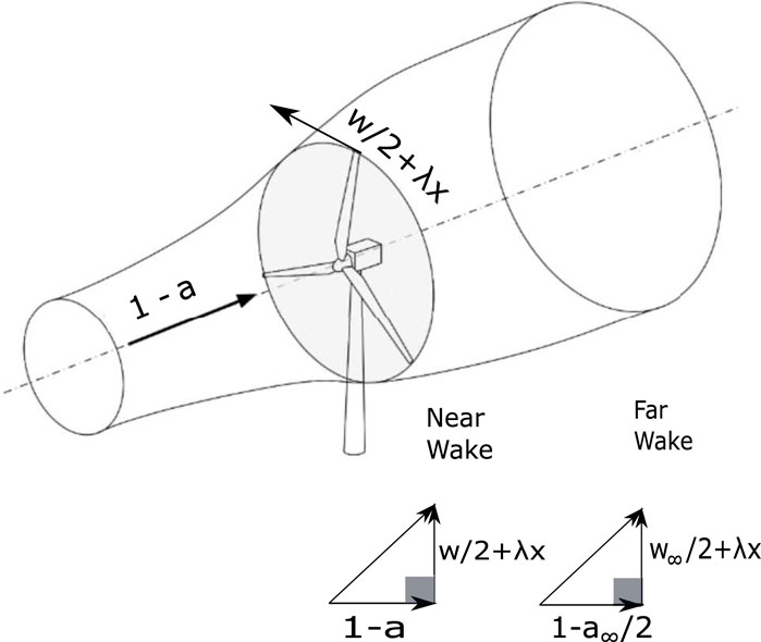
FIGURE 1. Perspective view of the actuator disc representation of a wind turbine rotor and the streamtube containing the flow that passes through the rotor. The arrows indicates the directions of the velocities which are normalized by the freestream velocity. The shaded circle shows the actuator disc. The velocity triangles are not to scale. Equation 14 gives p = (1 − a)/(λ + w/(2x)) and Equation 11 gives p∞ = (1 − a∞/2)/(λ + w∞/(2x)). The upper figure is adapted from https://openmdao.org/newdocs/versions/latest/examples/betz_limit.html.
The important early analyses of propeller performance by Betz (1921) and Goldstein (1929) in particular, assumed “light loading” whereby the velocities induced by the vortex structure representing the blades and wake, are small compared to the freestream velocity. As recounted in Okulov et al. (2015), this led to the “Betz-Goldstein” rotor whose optimal performance was associated with constant pitch of the helicoidal wake at the rotor. In other words, “the ideal flow [is] about rigid screw surfaces displaced axially backwards,” Betz (1921), page 8. On the next page, he states “We can, however, by foregoing strict mathematical accuracy, but without any error worth mentioning, so modify the laws [governing the flow] that they will also hold good for more heavily loaded propellers.” On the other hand, Goldstein (1929) states “The approximation that the trailing vortices form regular helices is equivalent to neglecting the contraction of the slipstream [for propellers], and is valid only for small values of the thrust coefficient.” It is noted that Goldstein acknowledged Betz for suggesting his study of optimal propellers, so the latter and later quote is a better summary of classical understanding. To the authors’ knowledge, the issue of optimality under arbitrary and general loading has not been fully addressed. It is also noted that Goldstein considered finite N whereas we restrict attention to ADs. It will be shown that “regular helices” can also occur for ADs with any loading.
Further development of AD theory after Betz and Goldstein, such as by Conway (1995; 1998), relaxed the light-loading assumption by using particular variations of vorticity and other fluid variables across the rotor and in the wake. van Kuik (2020), for example, considered the velocities at the rotor on the assumption that the disc loading or bound circulation, is constant. We note for later use that the disc loading is also proportional to the angular momentum of the fluid exiting the rotor. No study, however, has optimized turbine power production without first specifying the form of the loading. One of the challenges in doing this is that constancy of pitch immediately behind a lightly-loaded rotor guarantees constancy throughout the wake, but this is not the case for arbitrary loading. In order to undertake an optimization without specifying or assuming the loading, this investigation considers the far-wake in addition to the flow emerging from the rotor.
Our aim is to investigate optimal AD performance of horizontal-axis turbines as a function of λ. The light-loading approximation is relaxed and no assumptions are made about the velocity or vorticity distribution to start the analysis. Conditions for optimality are clarified, partly by considering the far-wake where the axial and circumferential velocities are related simply through the pitch. “Optimality” is taken to mean maximizing the power coefficient, CP, for any positive λ after first maximizing rotor torque for a fixed thrust. This is achieved using the calculus of variations, CoV, with Lagrange multipliers, as was done for propellers by Breslin & Andersen (1996) and Conway (1995). Propellers represent the inverse problem to turbines: the thrust is maximized for a given torque but the analysis is the same. It will be shown that CoV is easily implemented for turbine ADs and leads to important results with very little effort. Later work on propellers by Moreau et al. (2017) used a similar analysis. They also describe the history of these methods for propeller optimization. A variational method was used by Lopez-Garcia et al. (2012) to optimize hovering rotors. Section 9.3 of Sørensen (2015) describes the application of CoV to wind turbines but only for lightly-loaded rotors with small expansion, and without consideration of the far-wake. Bontempo and Manna (2022) used CoV to show that the Betz-Joukowsky limit gives the maximum performance of uniformly-loaded actuator discs in the presence of flow expansion but did not consider the effects of λ or the role of the vortex pitch.
In common with most turbine analyses, the AD equation for the torque is determined from conservation of angular momentum in the wake. The thrust is given by the Kutta-Joukowsky (KJ) equation as derived by Limacher and Wood (2021), hereinafter cited as LW. This equation has the circumferential velocity at the rotor, w, instead of the axial induction factor, a, that appears in the conventional thrust equation. Like the angular momentum equation but unlike the conventional thrust equation, the KJ equation is valid for any λ provided the vortex lines remain coincident with the streamlines.
The main novelty of this study is its determination of optimal rotor characteristics as a function of λ without making any assumptions about the nature of the loading. The BJ limit emerges as the global limit at sufficiently high λ. This result is not new but is important in understanding the changes to the flow at small λ. We also consider for the first time the far-wake’s role in determining optimality to minimize the assumptions made about the form of the flow through the rotor. Further, it is shown that for λ ≤ 2, optimal performance is constrained by the need to avoid the breakdown of the swirling, expanding wake.
The application of results derived for optimal ADs to real wind turbines is often a challenging task because it is not clear how the extension to even a lifting-line description can be done while maintaining the generality of arbitrary loading. Sørensen et al. (2022), for example, use the Goldstein light-loading results to derive the extracted power of a three-bladed rotor as a function of λ. We consdier the applicability of AD analysis to finite − N in Section 4.
The next section describes the CoV formulation starting with the simplest case of a lightly-loaded stationary rotor. This provides the lower bound on the distributions of the velocities and rotor loadings which change dramatically with λ. Section 3 presents and discusses the main results. Section 4 lists four important applications of the analysis to wind turbines, propellers and other thrust producers. The final section contains the conclusions. The Appendix derives an approximate and an exact solution for two special cases of the “disc loading equation,” derived in Section 2 and solved numerically to provide the results in Section 3. The closed-form solutions are used to assess the accuracy of the numerical ones.
2 Optimality via calculus of variations
The first part of the optimization problem is to maximize torque relative to thrust, both of which come from the lift for an ideal rotor with no viscous drag. For power-producing rotors (i.e. λ > 0) optimizing torque is equivalent to optimizing power which is the main goal of this study. We will, however, briefly consider stationary rotors as the λ ↓ 0 limit of the analysis. The relationship between the conventional power and torque coefficients, CP and CQ respectively, is CP = λCQ, from which it follows that
Thus maximizing torque on a stationary rotor, maximizes its power extraction as it begins to rotate.
2.1 Torque and thrust for an actuator disc
The conventional angular momentum equation is obtained using a cylindrical control volume (CV) centred on the axis of rotation and whose radius is large compared to the rotor radius, R. The inlet is well upwind of the rotor where w = 0, and the outlet is just downwind of it. For a circumferentially-uniform AD, The rotor torque Q is given by Equation (2.2) of Sørensen (2015) as:
where ρ is the fluid density, and U0 is the freestream velocity. x is the radius normalized by R, as are all lengths, and c = wx is the normalized angular momentum or disc loading which is often more useful than w. Throughout this paper, all velocities are normalized by U0. The upper limit on the integral can be any x ≥ 1 because w = 0 in this region. a is the usual axial induction factor at the rotor and it is emphasized that w is the azimuthal velocity immediately behind the blades. At the rotor, the azimuthal velocity is w/2 with the difference, w/2, coming from the bound vorticity of the blades. Equation 2 is valid for any distribution of w(x), and any expansion of the flow through the rotor.
For the same CV, the KJ equation for the thrust on an AD, T, is
LW derived Eq. 3 from an impulse analysis which shows that it is also exact for any distribution of w(x) and for any flow expansion. Equation 3 has an essential restriction: it requires alignment of the trailing vorticity with the streamlines in the wake, which will be assumed to hold throughout this analysis. Wood & Limacher (2021), hereinafter cited as WL, give the other seven assumptions required to derive (3). Equations 2, 3 must be augmented by consideration of the subsequent wake development as is done in deriving the BJ limit. It is important, therefore, to note that (2) holds everywhere in the wake, that is, from the near-to the far-wake in Figure 1, with a suitable adjustment to the upper limit on the integral, but (3) does not. Its general form in the near-wake includes the radial velocity, v, as explained by WL. Introducing v complicates the optimization, but fortunately v = 0 in the far-wake, which is considered in Section 2.4, after applying (2) and (3) at the rotor. Equations 2, 3 are given as (9.95) of Breslin & Andersen (1996) and used in a CoV determination of optimal propellers without considering the equivalent of significant flow expansion.
2.2 Lightly-loaded stationary rotors
The simplest case is a stationary rotor (λ = 0) for which the second term in (3) is zero. If the rotor is lightly-loaded, a is negligible. Combining Eqs 2, 3 leads to a simple CoV problem in terms of the Euler-Lagrange equation: to find the optimal distribution of w(x) given by
L is the Lagrange multiplier1 of the integrand in (3). Clearly, the solution is w = x/L, which maximizes Q = LT, and satisfies the boundary condition w(0) = 0. There is no need to consider a specific condition at x = 1 because the right side of (4) does not depend on dw/dx, see Section 1.4 of Wan (1993) and Section 1.5 of Komzsik (2020). Thus the wake, which will not expand significantly, is a vortex “core,” or more appropriately, a helicoidal vortex cylinder with constant (with x) pitch, p, defined as the streamwise co-ordinate of a point on the vortex divided by its helical angle; the precise from is derived in the next subsection. It is relevant to the later analysis to observe that p is directly related to the Lagrange multiplier as was noted by Breslin and Andersen (1996). It is further noted that if the maximization was of the circumferential force or lift, relative to thrust, then h = wx − Lw2x/2, and the optimal w becomes constant. This is only the start of a derivation of the optimality condition for wings which are also stationary, single-bladed rotors, but it does point to the close relationship between the analysis of lightly loaded wings and rotors. Both analyses, for example, ignore the induced axial velocity.
There are two reasons why this analysis is important for the study of optimal power-producing rotors. First, it gives the lower bound of w ∼ x as λ ↓ 0 which is very different from w ∼ 1/x associated with the BJ limit at high λ. Second, the inviscid expansion of flow with constant axial velocity and solid body rotation was analyzed in Section 7.5 of Batchelor (1967). To the authors’ knowledge, this is the only expanding flow that has exact equations for the velocities in the upstream and downstream regions. He showed that the expanded flow can break down through the appearance of negative velocities on the axis of rotation. Avoidance of breakdown is a further constraint on the present analysis and is considered in Section 2.6.
2.3 Rotors with arbitrary loading
At any λ, h is a function of w and a:
and the Euler-Lagrange equations for optimality are ∂h/∂a = ∂h/∂w = 0. The first requires w = 0 which is approached at high λ to give the BJ limit, and the second,
is applicable at all λ. The right side of (6) is LW’s Eq. 15 for the pitch of the trailing vorticity immediately behind the rotor, normalized by the blade radius. The pitch, as defined earlier, is also the tangent of the angle between the vortex lines and the plane of rotation. Thus, the connection between p and the Lagrange multiplier carries over to all λ and the Betz-Goldstein requirement that an optimal rotor has constant pitch is valid for arbitrary disc loading. It is, however, important to stress again that for light-loading with a ≈ 0, the optimal w remains linear in x at low values of λ. At high λ, λ ≫ w/x for most of the wake and the second term in Eq. 3 dominates. It will be shown that w ∼ 1/x for most x at high λ.
Setting p = L does not complete the optimality solution because a further relation is needed between a and w. This can be found either from the analysis of the far-wake in the next subsection, or by assuming helical symmetry at the rotor. Symmetry requires 2pa = c = wx as only w/2 is due to the trailing helical vorticity, and is strictly valid only for trailing vorticity of constant pitch and radius, as explained, for example, by WL. Symmetry and (6) lead to
which can be compared to Equation 58 of Okulov et al. (2015). Note that, at λ = 0, a = w2/2 for large p which makes its negligible. The equations for the velocities in (7) can be substituted into Eq. 2 to determine the torque. Multiplying by the angular velocity gives the extracted power which can be differentiated with respect to p to find the optimal power. This will not be done because it will be shown that helical symmetry is not a generally-valid assumption.
2.4 The far-wake with arbitrary loading
As an alternative to invoking helical symmetry at the rotor, which may be invalid for expanding flow, the far-wake can be analyzed. There, the vortex development is complete and helical symmetry will hold for any wake expansion. Quantities in the far-wake are identified by the subscript “∞”. The angular momentum equation has the same form as (2) but the thrust equation changes as noted above. The equations to be optimized are
where the equation for T is (25) of WL. R∞ is the non-dimensional radius of the far-wake. Thus
No special consideration of the dependence of R∞ on a∞ and w∞ is needed because Liebnitz’s rule for differentiating under an integral introduces no extra terms when dQ/dT = L∞ everywhere in the far-wake. Setting ∂h∞/∂a∞ = 0 gives the helical symmetry relation w∞x = L∞a∞, without a factor of 2 because w∞ is due entirely to the trailing vorticity. ∂h∞/∂w∞ = 0 results in
which, reassuringly, is also retrieved by removing a∞ from (9) using helical symmetry and considering only ∂h∞/∂w∞ = 0. Equation 10 again relates the Lagrange multiplier to the pitch. Since the values of torque and thrust cannot depend on the CV used to determine them, p = p∞ and, from 6, 7, 10, a∞ → a at high λ. This would prevent wake expansion and reduce power extraction. The approach of the far-wake pitch to the value given by (10) for maximizing the torque, must be constrained. One way of doing this is provided by the following considerations.
At any λ, the angular momentum or normalized circulation, c∞ = w∞x, is a monotonically increasing function of x, and the vortex core, where w is maximized, becomes smaller as λ increases. These results suggest that the far-wake approaches a “Joukowsky” wake in which all the positive vorticity (giving positive angular momentum and torque) is concentrated along the axis of rotation, and all negative (tip) vorticity in a cylindrical sheet at R∞, Okulov et al. (2015). The pitch of the tip vorticity is then
as the axial and circumferential velocities of the sheet must be the average of the wake velocities, 1 − a∞ and w∞ respectively, and the freestream values of unity and zero. The velocities in this definition of p∞ are shown in Figure 1. A “generalized Joukowsky” far-wake is now assumed for any λ: all negative (tip) vorticity is concentrated at the edge of the wake but the positive vorticity is an arbitrary, monotonically increasing function of radius. It is further assumed that: 1) the generalized wake is as close to the optimal as can be achieved when the tip vorticity is considered and 2) p∞ as given by (11) is the Lagrange multiplier. In other words, Eq. 11 is generally valid. With p∞ = p, the far-wake velocities are
CP,∞ and CT,∞ are given by
The reasons for limiting the pitch through Eq. 11 imply similar limitations for the flow exiting the rotor. If the wake does not expand significantly, which is the case for lightly loaded stationary rotors, then a in (6) should be replaced by a/2. WL showed that a just outside an expanding wake was comparable to that just inside, implying that no replacement of a should be made. Since a is negligible for lightly-loaded stationary rotors, it was decided that no change should be made to the form of a in (6). In contrast, the difference in w from inside to outside the far-wake occurs also at the rotor. Thus the pitch equation at the rotor is modified to
as indicated in Figure 1. The pitch Eqs 11, 14 are used for the remainder of this analysis. It is emphasized that these equations are approximations for most λ. In the Joukowsky wake at high λ, there will be no vorticity outside the core and beneath the tip vortex sheet, so that (11) will be exact. For the generalized Joukowsky wake, however, the vortex pitch within the wake will either be different from (11) as its axial velocity will be closer to 1 − a∞, or there will be a misalignment between vortex and streamlines and the thrust equations will be modified. No simple alternatives to the pitch equation appear possible, so we continue to use them as they are asymptotically correct and the main constraint at low λ comes from the need to avoid recirculation.
Finally, it has been mentioned that ending the CV anywhere between the rotor and the far-wake introduces the radial velocity v into the thrust equation as shown by Eq. 24 in WL: the T equation in (8) has an additional term v2/2 within the parentheses. In the absence of a relation between a, v, and w, this leads to an apparently useless additional optimization condition ∂h/∂v = 0 but the conditions on a and w are the same as on a∞ and w∞. This implies that the Lagrange multiplier is the vortex pitch throughout the wake of an optimal rotor and the pitch must be constant.
2.5 Combining the rotor and far-wake analyses
To solve the optimization problem for all λ, a∞ and w∞ must be related to a and w without using helical symmetry which may not hold hold if the wake expands significantly. One way to do this is to use the streamfunction, Ψ, defined as ∂Ψ/∂x = (1 − a)x anywhere in the wake and remove 1 − a using the ptich Eq. 14. This use of Ψ follows Batchelor’s (1967) study of expanding, swirling flow. He combined equations for the total energy and c = wx which depends only on Ψ by the principle of conservation of angular momentum. The relationship can be determined from Eq. 12 and then used to solve two ordinary differential equations (ODEs) behind the rotor:
for trial values of p, from which follow a and the thrust and torque. The present analysis reverses that used in Section 7.5 of Batchelor (1967). He established Ψ at the equivalent position to the rotor and then determined the velocities in the equivalent of the far-wake.
From Eq. 12, both c∞(x) and Ψ∞(x) are functions only of x2, which is easy to eliminate to derive the relationship between Ψ and c:
Differentiating (16) gives
and the equation for dc/dx is
This “disc loading” equation appears not to have a general closed-form solution. The exact solution for λp = 1/2 and the approximate solution for λ ≫ c/(2x2) are derived in the Appendix and used there to check the numerical solution which is now described.
2.6 Solving the disc loading equation for optimal power
The disc loading Eq. 18 for λ > 0 defines two boundary value (BV) ODEs that satisfy Ψ(1) = Ψ(cmax), c(1) = cmax = c∞(R∞), and Ψ(0) = c(0) = 0. As far as we could determine, the ODEs only have analytical solutions for the special cases described in the Appendix. BV numerical solvers are usually more difficult to implement than initial value solvers so the Matlab variable step length Runge-Kutta routine ode113 was used to integrate dc/dx at all λ for trial values of R∞ and p. To avoid numerical singularities at x = 0, the integration was started from x0 = 0.001 for all but the highest λ in Table 1 for which x0 = 0.0001. The initial value of c was
where c0 and c2 were determined from Eq. 18:
Integration was terminated at x = xend defined by Ψ(xend) = Ψ(cmax). If |1 − xend| > 0.001 the solution was rejected. This rejection was important because some values of p and R∞ gave CP,∞ > 16/27. High CP, however, always caused xend > 1 to “lower” CP by increasing the rotor radius. Using Ψ to terminate the solution was found to give very similar results to the use of c. Checks of the numerically determined a and c against the analytic solutions for the special cases of λp = 1/2 at low λ and λx ≫ c/x at high λ are described in the Appendix. The numerical values were found to be very accurate except for a at very small values of x.
Because some far-wake equations gave CP > 16/27, the search for optimal performance could not be based on finding the value of p that maximized far-wake CP for a trial value of R∞. Instead, for each λ, a range of p and R∞ was used to find c(Ψ) for the far-wake from Eq. 12. There was no rejection of solutions for which CP > 16/27 from (13) so as not to bias the search for optimality. The ODEs in (15) were complemented by ODEs for CP and CT and all equations were solved concurrently. The solutions were rejected if the relative tolerance |(CP − CP,∞)/CP,∞| > 0.001. The tolerances used in solving the ODEs were at least two orders of magnitude smaller. The maximum CP for each λ was found by inspection by incrementing R∞ and λp in steps of 0.0001. A typical example of the search for optimal values, at λ = 4 is shown in Figure 2 which is discussed in detail in the next section.
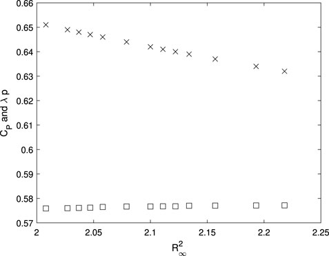
FIGURE 2. Iteration of the power coefficient (□) and λp (×) for λ = 4.
2.7 Detecting flow breakdown
Seeking the optimal solutions at small λ resulted in large w as x → 1. This may lead to flow breakdown in a way that the present analysis does not consider. Wake breakdown is analyzed in Section 6.6 of Sørensen (2015). He assumed a Joukowsky wake for low λ but, as shown in Section 2.3, this is not valid for an optimal rotor. Without prescribing the wake, it is still possible to follow Sørensen (2015) in determining the significance of high w by using the swirl number, S, defined as the ratio of the fluxes of angular and axial momentum. It is commonly held that swirling flow will break down at a threshold value S ≈ 0.5, e.g. Vignat et al. (2022). In the present flow, S in the far-wake is given by
For optimal rotors, the equation for S∞ can be approximated as
ΔCT is the mass flux which is also the upwind momentum flux entering the CV. Since ΔCT > 0, it follows that S∞ < p which restricts the range of λ for which breakdown is possible to λ⪅2.
Section 2.2 showed that a is small and w ∼ x at low λ, and mentioned that the expansion of this flow is analyzed in Section 7.5 of Batchelor (1967). His Equations (7.5.22) and (7.5.23) give the equivalent far-wake velocities as
in the present notation. a is constant, and J0(.) and J1(.) are Bessel functions of the first kind of order zero and one respectively. The coefficient A is given by
Breakdown starts when U∞(x = 0) = 0, i.e. when A = 1. This defines the critical p as a function of R∞ and limits expansion to
3 Results and discussion
The optimal power and thrust from the analysis in subsection 2.6 are shown in Figure 3 along with the CP results from Glauert’s (1935) optimization. The current results are listed in Table 1. All the computed CP and CT asymptote to the BJ values at high λ. Figure 3 can be compared to the “Betz-Goldstein” results in Figure 30 of Okulov et al. (2015), Figure 8 and Figure 9 of Vaz & Wood (2016), and Figure 6.14 of van Kuik (2018). Most previous determinations of CP closely follow Glauert’s results.
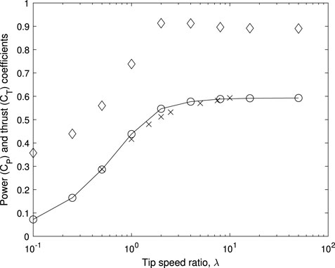
FIGURE 3. Optimal actuator disc power and thrust. × is CP from Glauert (1935). The circles are CP, the diamonds are CT from Table 1. The solid line is for visual aid only. Note that CP asymptotes to the BJ limit of 16/27 and CT to the corresponding limit of 8/9.
Figure 2 plots the progress in the search for optimal power and thrust as the far-wake radius is altered. It indicates the flatness of the region of peak performance, which occurs at all λ, but shown for λ = 4 only. In other words, there is a wide range of p and R∞ where CP does not vary significantly from the optimal value. The results plotted are the current maximum CP for the search in units of 0.0001 for
Figures 4, 5 plot the distributions of a and w respectively. Equation 2 requires that no torque is extracted from the streamline on the axis of rotation, x = 0, and (3) shows the same is true for thrust. Therefore a(x = 0) = w(x = 0) = 0 for any λ. Similarly, Eq. 12 requires a∞(x = 0) = w∞(x = 0) = 0 for any λ. The change in a and w with λ is dramatic. At very small λ, a ∼ x2 and w ∼ x per the light-loading limit for stationary rotors, but a → 1/3 and w ∼ 1/x at high λ for consistency with the BJ limit which can be seen from Figure 3 to be the high − λ limit.
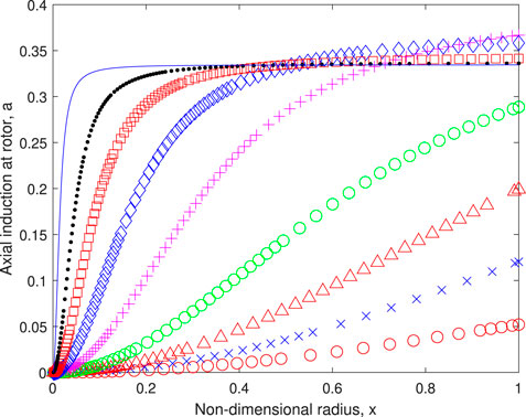
FIGURE 4. The axial induction factor at the rotor. Symbols are defined in Table 1.
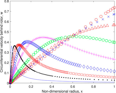
FIGURE 5. The circumferential velocity at the rotor. Symbols are defined in Table 1.
The tests of helical symmetry - the extent to which the equation 2pa = wx = c holds behind the rotor - in Figure 6 are the most important results of this section. They are also the most unexpected as helical symmetry is violated at low λ and then becomes increasingly accurate as λ increases for sufficiently large x. There are two main inferences from this behaviour. First, the large variation justifies the complicated analysis of the previous section: assuming helical symmetry at the rotor makes the determination of optimal performance straightforward. Secondly, the conventional thrust equation
follows from (3) only if 2pa = c = wx. The listing of
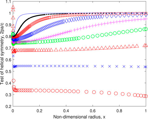
FIGURE 6. Test of helical symmetry. Symbols are defined in Table 1.
The results in Figure 6 near x = 0 at low λ are affected by the small values of a and some are unreliable as demonstrated in the Appendix. On the other hand, at high λ where the Betz-Joukowsky limit requires a = 1/3, that is a constant, helical symmetry can only occur in the region where c is constant. In other words, the lack of helical symmetry at small x must be a genuine expression of the wake model. The series expansion of Eq. 19 at x = 0 with the coefficients from Eq. 20, gives the limiting form of c(x), and of a(x) from (15):
Thus
The limiting values, listed in Table 1, are in excellent agreement with the majority of the small − x results in Figure 6. We note also that the asymptotic form of c, Eqs 19, 20, and a from (26) agree with the small − x behaviour of the exact solution for λp = 1/2, Eq. (A7). Having the largest departures from helical symmetry when λ ↓ 0 conflicts with the expectation of minimal expansion of the wake for a stationary rotor which implies the validity of helical symmetry. From (27), helical symmetry is possible at small λ only if λp = 1 which implies p → ∞ as λ ↓ 0 and minimal a. As mentioned in subsection 2.5, an alternate low − λ model with small expansion does not seem possible. Figure 5 shows the “core” of the trailing vorticity shrinks with increasing λ so the lack of helical symmetry eventually becomes of little dynamical importance but it can never be valid for the whole rotor flow as λp < 1 as noted previously.
a∞ and 2a are plotted against the streamfunction, Ψ, in Figure 7. a∞ = 2a is normally assumed in deriving the one-dimensional equations leading to the BJ limit, but it is clear from the figure that the approximation becomes valid only at high λ as suggested by the pitch Eqs 11, 14 when λx ≫ w. At low λ, the approximation, like helical symmetry, is in considerable error. The failure of helical symmetry at low λ has been highlighted as a major finding of this analysis. There are two further aspects of it, related to p, that are worth commenting on. From Eq. 14 and the coincidence of streamlines and vortex lines, we have
behind the rotor. Ωz and Ωθ are the axial and circumferential vorticities, respectively, and v is the radial velocity. For constant p, ∂v/∂z ∼ ∂c/∂z whenever pa is a constant multiple of c. Thus v is maximized at the rotor both at low and high λ when c becomes independent of x for most of the wake. In general, ∂c/∂x > 0 and the streamtube in Figure 1 expands more behind the rotor than ahead of it. This is consistent with the general result that 2a < a∞ from Figure 7. In the far-wake, ∂v/∂z = 0 ∀ λ, so the coincidence of vortex lines and streamlines implies that p is constant across the wake as helical symmetry must hold. This result does not avoid the need for CoV because it is insufficient to establish optimality.
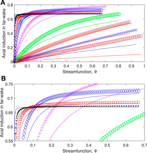
FIGURE 7. The far-wake velocity with the symbols defined in Table 1 compared to 2a shown as a solid line of the same colour. (A) All results. (B) Results at high λ. Note that the results for λ = 1 are not shown for clarity. Symbols are defined in Table 1. The 2a results for λ = 50 cannot be distinguished from the lines showing a∞.
The second aspect is also an important one that has been left until the evidence has been marshalled. The defining feature of the present analysis is that no a priori assumptions have been made about the dependence of the disc loading on x or the forces on the rotor. The 1 − a term in Equation 28 shows that p, which defines the flow direction at the rotor, is normal to the force acting on the streamtube with axial velocity 1 − a, and so the disc loading is due to a Kutta-Joukowsky force.
4 Some applications of the analysis
We briefly describe some applications and implications of the analysis:
4.1 Wind turbines at low tip speed ratio
Most large wind turbines operate at high λ where the current analysis conforms to the Betz-Joukowsky performance limits. As turbine size decreases, however, keeping a high λ means increasing in the rotational speed which can lead to problems with noise and safety, Wood (2011). Small turbine operation at low λ has been studied by only a few researchers, e.g. John et al. (2020) and Bourhis et al. (2022), and a thorough understanding of them has not been developed. Those experiments used high solidity rotors as a way to ensure fast starting. For λ ≤ 2, John et al. (2020) found maximum power coefficients considerably lower than the current values suggesting that an optimization of blade design would be beneficial. Sørensen et al. (2022) used prescribed loadings to investigate computationally the λ − dependence of the power output of a three-bladed turbine. The extracted power was less than given by the present analysis, as it should be, but do not report any evidence of approaching recirculation. The current analysis suggests that avoiding recirculation is important in the optimization but it will require further investigation to see how this is affected by having a finite N.
4.2 The constancy of vortex pitch
An important result from the present analysis is that p remains constant throughout the wake of an optimal AD at any λ. It is reasonable to extrapolate this result to rotors with finite N which can be analyzed using blade element/momentum theory. Then, Equations 2, 3 must be modified using “finite blade functions,” FBFs, which are also needed to determine the velocities at the blades in terms of the circumferentially-averaged velocities. FBFs are normally assumed to be given by Prandtl’s tip loss factor but more general forms can be derived from the Kawada-Hardin (KH) solution to the velocity field of an infinite helical vortex of constant p and radius, Kawada (1936), (1939), Hardin (1982), and Fukumoto et al. (2015). There are no other known, closed-form solutions for the velocity field of helical vortices. Simple and accurate approximations to the KH solutions are described in Wood et al. (2021) and were used to analyse the effects of low λ by Wood et al. (2016) and Vaz & Wood (2016), and blade sweep by Fritz et al. (2022). Wood (2021) showed that the expansion of the trailing vortices in the wake of a real turbine is easily accounted for in the approximations to the KH equations. The present analysis implies that the remaining restriction of the KH equations to constant p is not significant.
4.3 Moving wind turbines
If a turbine is mounted on a a land vehicle, Gaunuaa et al. (2009) and Section 3.6 of Sørensen (2015), or a ship, Connolly and Crawford (2022), it is possible under some circumstances to produce more power than required to move the turbine. Consider the simplest and most favourable case of a turbine moving at constant velocity Ut into a constant headwind of U0. The power is proportional to
4.4 Propellers and other thrust producers
As noted in the Introduction, the current work is based on the CoV study of propellers by Breslin and Anderson (1996). Their analysis was limited, however, to light disc loading with small wake contraction, as was Goldstein’s (1929). The current analysis can be inverted to apply to propeller ADs of arbitrary loading by maximizing the thrust for a given torque because the inversion does not alter the CoV analysis. The contraction of typical propeller wakes is much less than the expansion of typical wind turbine wakes, but a full AD analysis should clarify the accuracy of assuming light loading. Propeller performance is usually characterized in terms of the advance ratio J = π/λ. High J, therefore, corresponds to low λ so the current results at low λ suggest the need to revisit high-J propeller performance.
Many other thrust producers have an energy cost. An example is tilted-pad thrust bearings, e.g. Liu & Mou (2012), where the thrust is the bearing load and the torque gives the energy lost to the bearing. A CoV analysis to minimize the energy cost could be valuable.
5 Conclusion
This analysis considered the optimal performance of actuator disc (AD) models of horizontal-axis turbines. The optimization used the circumferentially-uniform equations for angular momentum and the Kutta-Joukowsky equation for thrust, both derived initially for a control volume ending immediately behind the rotor. The thrust equation is valid only if the vortex lines and streamlines are coincident in the wake.
The maximum power at any tip speed ratio (λ) was found from a straightforward application of the calculus of variations as has been done previously for lightly-loaded propellers, but not for turbines with arbitary loading. The angular momentum and thrust equations are valid for any distribution of induced axial and circumferential velocities and any amount of wake expansion. For the first time, the conditions for an optimal far-wake were established and then used to derive the disc loading equation for the rotor. This avoided any a priori assumptions about the flow through the rotor. The link between rotor torque and thrust is the pitch of the trailing vorticity. We showed that the optimal pitch was constrained by the vorticity distribution in the wake. The resulting, approximate Eqs 11, 14 for the pitch were used for the rest of the analysis.
It was found that the conventional equation for thrust involving only the axial velocity, is incorrect at low λ but becomes asymptotically valid as λ → ∞. In common with previous studies, the familiar Betz-Joukowsky limit was the global limit on turbine performance. By starting the optimization with the far-wake, we avoided using helical symmetry at the rotor. Surprisingly, this symmetry relation between the axial and circumferential velocities was invalid at low tip speed ratio where the wake expansion was small but became accurate only at large λ. The failure of helical symmetry is closely linked to the inaccuracy of the conventional thrust equation and the finding that the streamtube expands more behind the rotor than ahead of it.
For λ⪅2, the optimization was constrained by the need to avoid flow breakdown – the axial velocity going to zero on the centreline in the far-wake. An analytic solution for a related, expanding, inviscid flow with vorticity, was used to determine a swirl number criterion for breakdown.
Using the calculus of variations shows that the link between optimal torque and thrust is the pitch of the wake vorticity and that optimality requires constant pitch across the wake. These results hold for any loading of the disc and so extend the classical findings of Betz and Goldstein that optimality requires constant pitch for lightly loaded discs. Since the torque and thrust must be unaltered by moving the end of the control volume to the far-wake, we deduce the valuable result that pitch is also constant across the far-wake and equal to the pitch behind the rotor. The argument at the end of Section 2.4 implies that the pitch in an optimal turbine wake is everywhere constant. This justifies a more general determination of finite-blade effects than the common use of Prandtl’s tip loss factor, as explained in the previous Section. The importance of vortex pitch for optimal rotors extends to its setting the radius of the vortex core, the region where the circumferential velocity w increases from zero at the axis to its maximum value. The core radius decreases monotonically with λ to become negligible as the Betz-Joukowsky limit is approached.
It was proved in Section 2.2 that an optimal, lightly-loaded, stationary rotor, has w is proportional to the radius, so the circulation is quadratic in radius whereas the circulation and the axial velocity are nearly constant in the Joukowsky wake of an optimal rotor at infinite λ. Optimal rotors clearly cannot have a Joukowsky wake at low tip speed ratios. The wake at all tip speed ratios, however, can be classified as a “generalized Joukowsky” wake as the circulation increases monotonically with the radius until the edge of the wake where it goes to zero.
Data availability statement
The raw data supporting the conclusions of this article will be made available by the authors, without undue reservation.
Author contributions
The study was conceived by DW who also did the numerical analysis. MH contributed to the literature review and the solution of the ODE in the Appendix. The mathematical analysis was shared.
Funding
DW’s contribution was supported by the Natural Sciences and Engineering Research Council Discovery Program.
Conflict of interest
The authors declare that the research was conducted in the absence of any commercial or financial relationships that could be construed as a potential conflict of interest.
Publisher’s note
All claims expressed in this article are solely those of the authors and do not necessarily represent those of their affiliated organizations, or those of the publisher, the editors and the reviewers. Any product that may be evaluated in this article, or claim that may be made by its manufacturer, is not guaranteed or endorsed by the publisher.
Footnotes
1Lagrange multipliers are usually denoted by the symbol (λ) we use for the tip speed ratio.
Appendix: Exact and approximate solutions of the disc loading equation
This Appendix describes the checks made on the accuracy of the numerical solution of Equation 18 using the closed form solution for λp = 1/2 and an approximate solution for λx ≫ c/x that are now derived. Equation 18 is
which separates approximately when λx ≫ c/x and exactly when λ = 0. We ignore the latter case as not relevant and derive the approximate solution. Then (Equation 18) reduces to
and so
where C is the constant of integration. Applying c = cmax at x = 1 gives
A typical comparison of a, c and pa/c is shown in Figure 8 for λ = 8 where (A2) should be accurate for sufficiently large x. It is concluded that the numerical integration is accurate at high λ when the poor accuracy in the helical symmetry test for very small x is discounted.
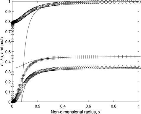
FIGURE 8. Comparison of the numerical determination of a, △, λc, + and pa/c, ○, at λ = 8 to the analytic approximation, Equation (A2).
Equation 18 is not separable when λ ≠ 0 and λx ≈ c/x. Its general form can be transformed to an Abel equation of the first kind using the substitution
to yield
where the coefficients are
p1 = 1/(2(1 − λp)), and p2 = λ/(p(1 − λp)). When p1 = 1 or λp = 1/2, a simple, exact solution can be obtained. Equation (A4) reduces to
whose solution according to Mathematica is
where erf(.) is the error function. The constant of integration in Equation (A7) was set to zero to make a(0) = 0. This leads to a direct relationship between R∞ and λ from imposing c(1) = cmax which is likely to be a feature of any exact solution. Such a relationship would be highly desirable in the general search for optimality except for λ ≤ 2 where optimality is constrained by flow breakdown. For λp = 1/2 the equation for the far-wake radius is
This is a very interesting result because R∞ increases without bound as λ increases. The case of λp = 1/2 deserves further study which we postpone as it is not directly relevant to the optimization of rotor power.
Figure 9 compares the exact solution of Equation (A7) to the numerical determination of c for λ = 0.5 where (A8) gives
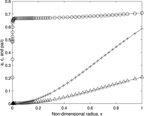
FIGURE 9. Comparison of the numerical determination of a, △, c, + and pa/c, ○, at λ = 0.5 and λp = 1/2 to the analytic solution, Equation (A7), shown as the solid lines.
The cubic polynomial in (A4) has two real roots at c∗2 = 2(1 − λp)/(1 − 2λp) and one at c∗0 = 2p(1 − λp)/(p + 2λx2) which again shows the equation is separable only at λ = 0. Using the method in Section 4-1 of Murphy (2011), (A4) can be reduced to the standard Abel equation as
where
References
Bontempo, R., and Manna, M. (2022). Optimal distribution of the disk load: Validity of the betz–joukowsky limit. AIAA J. 1-6, 4868–4873. doi:10.2514/1.j061639
Bourhis, M., Pereira, M., Ravelet, F., and Dobrev, I. (2022). Innovative design method and experimental investigation of a small-scale and very low tip-speed ratio wind turbine. Exp. Therm. Fluid Sci. 130, 110504. doi:10.1016/j.expthermflusci.2021.110504
Breslin, J. P., and Andersen, P. (1996). Hydrodynamics of ship propellers. Cambridge University Press.
Connolly, P., and Crawford, C. (2022). Analytical modelling of power production from un-moored floating offshore wind turbines. Ocean. Eng. 259, 111794. doi:10.1016/j.oceaneng.2022.111794
Conway, J. T. (1995). Analytical solutions for the actuator disk with variable radial distribution of load. J. Fluid Mech. 297, 327–355. doi:10.1017/s0022112095003120
Conway, J. T. (1998). Exact actuator disk solutions for non-uniform heavy loading and slipstream contraction. J. Fluid Mech. 365, S0022112098001372–267. doi:10.1017/s0022112098001372
Fritz, E. K., Ferreira, C., and Boorsma, K. (2022). An efficient blade sweep correction model for blade element momentum theory. Wind Energy 1-18. doi:10.1002/we.2778
Fukumoto, Y., Okulov, V. L., and Wood, D. H. (2015). The contribution of Kawada to the analytical solution for the velocity induced by a helical vortex filament. Appl. Mech. Rev. 67 (6), 060801. doi:10.1115/1.4031964
Gaunaa, M., Øye, S., and Mikkelsen, R. F. (2009). “Theory and design of flow driven vehicles using rotors for energy conversion,” in European wind energy conference and exhibition (Marseille, France: EWEC).
Glauert, H. (1935). “Airplane propellers,” in Aerodynamic theory (Berlin, Heidelberg: Springer), 169–360.
Hardin, J. C. (1982). The velocity field induced by a helical vortex filament. Phys. Fluids 25, 1949–1952. doi:10.1063/1.863684
John, I. H., Vaz, J. R., and Wood, D. (2020). Aerodynamic performance and blockage investigation of a cambered multi-bladed windmill. J. Phys. Conf. Ser. 1618 (7), 042003. doi:10.1088/1742-6596/1618/4/042003
John, I. H., and Wood, D. (2021). “The aerodynamics of water pumping windmills,”. Small wind and hydrokinetic turbines. Editors P. D. Clausen, J. Whale, and D. Wood, 169.
Kawada, S. (1939). Calculation of induced velocity by helical vortices and its application to propeller theory. Rep. Aeronaut. Res. Inst. Tokyo Imp. Univ. 14 (2–57).
Kawada, S. (1936). Induced velocity by helical vortices. J. Aeronautical Sci. 3, 86–87. doi:10.2514/8.141
Komzsik, L. (2020). Applied calculus of variations for engineers. Third Edition. Boca Raton, FL: CRC Press.
Limacher, E., and Wood, D. (2021). An impulse-based derivation of the Kutta–Joukowsky equation for wind turbine thrust. Wind Energy Sci. 6, 191–201. doi:10.5194/wes-6-191-2021
Liu, S., and Mou, L. (2012). Hydrodynamic lubrication of thrust bearings with rectangular fixed-incline-pads. J. Tribol. 134, 024503–1. doi:10.1115/1.4006022
Lopez-Garcia, O., Cuerva, A., and Esteban, S. (2012). Use of calculus of variations to determine the shape of hovering rotors of minimum power and its application to micro air vehicles. Proc. Institution Mech. Eng. Part G J. Aerosp. Eng. 226 (5), 574–588. doi:10.1177/0954410011411636
Mancas, S. C., and Rosu, H. C. (2016). Integrable Abel equations and vein’s Abel equation. Math. Methods Appl. Sci. 30 (6), 1376–1387. doi:10.1002/mma.3575
Mikkelsen, R. F., Sarmast, S., Henningson, D., and Sørensen, J. N. (2014). Rotor aerodynamic power limits at low tip speed ratio using CFD. J. Phys. Conf. Ser. 524 (1), 012099. doi:10.1088/1742-6596/524/1/012099
Moreu, J., Epps, B. P., Valle, J., Taboada, M., and Bueno, P. (2017). Variational optimization of hydrokinetic turbines and propellers operating in a non-uniform flow field. Ocean. Eng. 135, 207–220. doi:10.1016/j.oceaneng.2017.02.018
Okulov, V. L., Sørensen, J. N., and Wood, D. H. (2015). The rotor theories by Professor Joukowsky: Vortex theories. Prog. Aerosp. Sci. 73, 19–46. doi:10.1016/j.paerosci.2014.10.002
Sørensen, J. N. (2015). General momentum theory for horizontal Axis wind turbines. Heidelberg: Springer International Publishing. doi:10.1007/978-3-319-22114-4
Sørensen, J. N., Okulov, V., and Ramos-García, N. (2022). Analytical and numerical solutions to classical rotor designs. Prog. Aerosp. Sci. 130, 100793. doi:10.1016/j.paerosci.2021.100793
van Kuik, G. A. M. (2020). On the velocity at wind turbine and propeller actuator discs. Wind Energy Sci. 5 (3), 855–865. doi:10.5194/wes-5-855-2020
van Kuik, G. A. M. (2018). The fluid dynamic basis for actuator disc and rotor theories. Amsterdam: IOS Press.
Vaz, J. R., and Wood, D. H. (2016). Performance analysis of wind turbines at low tip-speed ratio using the Betz-Goldstein model. Energy Convers. Manag. 126, 662–672. doi:10.1016/j.enconman.2016.08.030
Vignat, G., Durox, D., and Candel, S. (2022). The suitability of different swirl number definitions for describing swirl flows: Accurate, common and (over-) simplified formulations. Prog. Energy Combust. Sci. 89, 100969. doi:10.1016/j.pecs.2021.100969
Wan, F. Y. M. (1993). Introduction to the calculus of variations and its applications. Boca Raton, FL: CRC Press.
Wood, D. H. (2015). Maximum wind turbine performance at low tip speed ratio. J. Renew. Sustain. Energy 7 (5), 053126. doi:10.1063/1.4934805
Wood, D. H., Okulov, V. L., and Bhattacharjee, D. (2016). Direct calculation of wind turbine tip loss. Renew. Energy 95, 269–276. doi:10.1016/j.renene.2016.04.017
Wood, D. H., Okulov, V. L., and Vaz, J. R. P. (2021). Calculation of the induced velocities in lifting line analyses of propellers and turbines. Ocean. Eng. 235, 109337. doi:10.1016/j.oceaneng.2021.109337
Wood, D., and Limacher, E. (2021). Some effects of flow expansion on the aerodynamics of horizontal-axis wind turbines. Wind Energy Sci. 6 (6), 1413–1425. doi:10.5194/wes-6-1413-2021
Keywords: actuator disc, horizontal-axis turbines, wind turbines, optimization, maximum power, calculus of variations, finite bade number, tip speed ratio
Citation: Wood DH and Hammam MM (2022) Optimal performance of actuator disc models for horizontal-axis turbines. Front. Energy Res. 10:971177. doi: 10.3389/fenrg.2022.971177
Received: 16 June 2022; Accepted: 30 September 2022;
Published: 02 November 2022.
Edited by:
Stefano Leonardi, The University of Texas at Dallas, United StatesReviewed by:
Davide Astolfi, University of Perugia, ItalyUmberto Ciri, University of Puerto Rico at Mayagüez, Puerto Rico
Copyright © 2022 Wood and Hammam. This is an open-access article distributed under the terms of the Creative Commons Attribution License (CC BY). The use, distribution or reproduction in other forums is permitted, provided the original author(s) and the copyright owner(s) are credited and that the original publication in this journal is cited, in accordance with accepted academic practice. No use, distribution or reproduction is permitted which does not comply with these terms.
*Correspondence: David H. Wood, ZGh3b29kQHVjYWxnYXJ5LmNh