Integrated stability control for a vehicle in the vehicle-to-grid system on low adhesion coefficient road

For the vehicle-to-grid system, the dynamic performance of the vehicle in the transportation system is quite crucial. The stability of the vehicle is the basis of the whole system. Compared to the traditional vehicle, the vehicle with a torque distribution system allows the vehicle to have a better dynamic performance. The torque distribution method has attracted a lot of attention from researchers. Most of the current work focuses on the vehicle on the concrete road. To improve the vehicle lateral stability in the critical work condition, the nonlinear reference model and vehicle dynamic model with 8 degrees of freedom are established based on the vehicle dynamic theory. An integrated active front steering (AFS) and direct yaw control (DYC) controller are designed based on LQR (Linear quadratic regulator) and vehicle stability phase portrait. To evaluate the performance of the vehicle on the road with a relatively low adhesion coefficient. The double lane-change and fishhook maneuver are chosen as the work condition. The steering angle, wheel torque, vehicle routine, phase portrait track, and yaw rate are calculated and compared. The simulation result validates the effectiveness of the proposed integrated AFS and DYC control method. The stability of the vehicle on the low adhesion coefficient road can lay a good foundation of the vehicle-to-grid system.

Introduction

The Electric vehicle (EV) shows a promising future due to its advantage in energy conservation and environment protection. The EV with wheel motors has superior performance in advanced chassis control algorithms because of its simplified chassis and independent driving torque. The independent driving torque on the vehicle wheels allows the vehicle to have a better ability on torque vectoring (TV) control. The TV control can improve the dynamic performance of the vehicle according to the driver’s attention without significantly damaging its speed.

Normally, the TV or differential braking control (DBC) is integrated with the traditional steering system to improve vehicle performance (Soares et al., 2018) (Chen et al., 2017). Based on the coordination of active front steering (AFS), direct yaw control (DYC), and TV control, an integrated control algorithm is provided to maintain the vehicle stability during extreme work conditions (Aouadj et al., 2020); (Li et al., 2019). Besides lateral stability, some researchers also consider roll stability, the TV control is combined with the AFS to enhance the yaw and roll stability of a coach (Zheng et al., 2018). Usually, the torque control distribution algorithm is made up of 2 or 3 layers (Khalfaoui et al., 2018). The stability judgment, slip rate calculation, torque allocation, and steering angle are determined in the upper layer, while the lower layer conducts the torque inverting. The plane phase method can represent the nonlinear characteristics, therefore, it is widely used in vehicle stability judgment. The plane phase method can be classified according to the state variable used in the plane phase, including sideslip angle-sideslip angular velocity (Inagaki et al., 1994), yaw rate-sideslip angle (Ono et al., 1998), and front-rear tire sideslip angle (Bobier and Gerdes, 2013). Different torque control algorithms, such as fuzzy control (Boada et al., 2005), PID (Liu et al., 2019), LQR (Linear quadratic regulator) (Dai et al., 2019), MPC (Model predictive control) (Zhang and Wu, 2016), and sliding-mode control (Truong et al., 2013) are initiated to allocate the needed torque during the steering process. For the torque distribution process, even distribution, generalized inverse matrix, and least square are the commonly used algorithms (Xu et al., 2019).

Plenty of works have been done in this area, most of the current research focuses on vehicles running on the regular road with an adhesion coefficient of around 0.8. With a lower adhesion coefficient, lower friction force can be provided by the road surface, thus, the easier the vehicle runs out of control. To deal with the critical situation of the passenger car, an 8 DOFs vehicle and 2 DOFs reference model are established and validated by the result of Carsim. According to the stability phase portrait and LQR method, an integrated AFS and DYC controller is designed. The effectiveness of the controller is proved by the simulation of two critical maneuvers on low friction adhesion road. The results show the overall improvement of the vehicle’s lateral stability.

Vehicle dynamic model

To investigate the differential torque steering control algorithms, the vehicle dynamic model is established based on the vehicle dynamic theory. For an operating vehicle, lots of freedom exists in the whole system, the simplification must be done based on the researchers’ focus. Normally, a 2 DOF model is established as the reference model and the multiple DOF model such as the 8, 10, or 14 DOF model is established to verify the torque distribution algorithms (Jaafari and Shirazi, 2016); (Goodarzi et al., 2011). In this case, 2 and 8 DOF vehicle dynamic models are built. Since the 8 DOF model is much more complicated than the 2 DOF model, the 8 DOF model is introduced first. The 8 DOF model is combined with the vehicle body, wheel, motor, and tire model.

Vehicle body model

For the vehicle dynamic model, the 4 out of 8 DOFs are for the vehicle body and the remaining 4 DOFs are for the wheel rotations. The 4 DOFs for the vehicle body model are the motion of longitudinal, lateral, yaw, and roll (Figure 1). The four motions can be identified as Eqs 1–4, the symbol and vehicle parameters used in these equations are shown in Table 1.

$m\left({\dot{v}}_x-v_y\gamma \right)+m_s{h}_s\gamma \dot{\varphi }={\displaystyle {\sum }_{i=1}^4{F}_{xi}}-\frac{1}{2}{C}_{d}A\rho v_x^2-mgf(1)$

$m\left({\dot{v}}_y+v_x\gamma \right)-m_s{h}_s\ddot{\varphi }={\displaystyle {\sum }_{i=1}^4{F}_{yi}}(2)$

$I_x\ddot{\varphi }-m_s{h}_s\left({\dot{v}}_y+\gamma v_x\right)-I_{xz}\dot{\gamma }=m_{s}g{h}_s\varphi -\left(K_f+K_r\right)\varphi -\left(C_f+C_r\right)\dot{\varphi }(3)$

$I_z\dot{\gamma }-I_{xz}\ddot{\varphi }=M+\left(F_{y1}+F_{y2}\right)L_f-\left(F_{y3}+F_{y4}\right)L_r(4)$

$M=\frac{L_w}{2}\left(F_{x2}+F_{x4}-F_{x1}-F_{x3}\right)(5)$

FIGURE 1

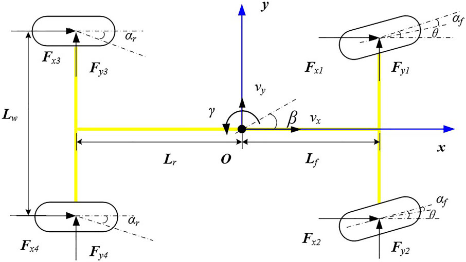
FIGURE 1. Diagram of the 8DOF model.

TABLE 1

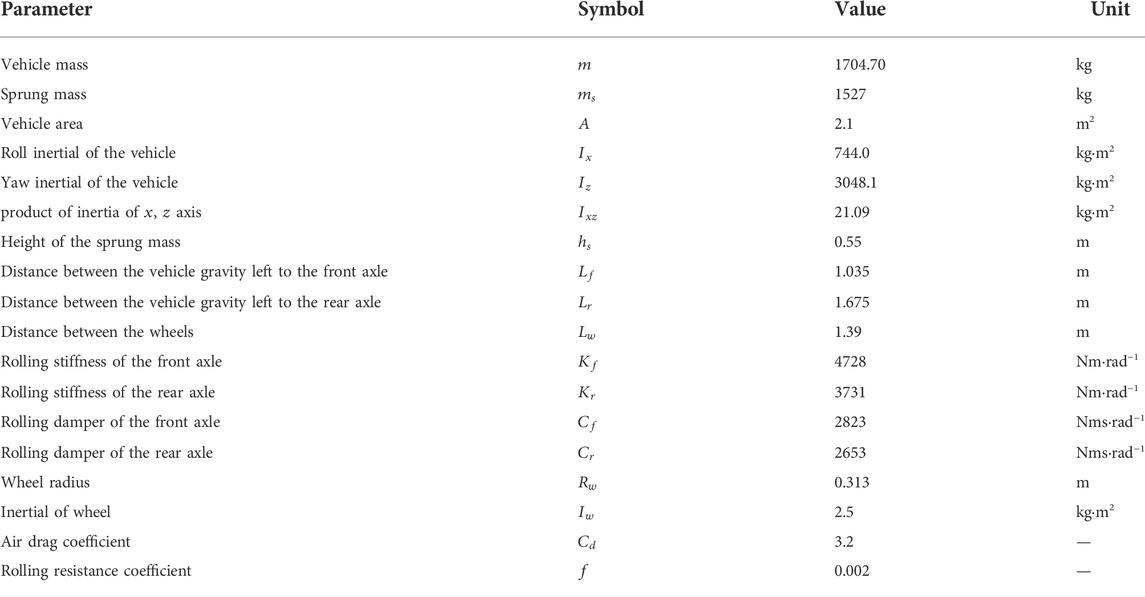
TABLE 1. Vehicle parameters.

Where, $v_x$ and $v_y$ are the longitudinal and lateral speed of the vehicle, $\gamma$ means the yaw rate, $\varphi$ is the roll angle, $F_{xi}$ and $F_{yi}$ are the longitudinal and lateral force of the four wheels in the coordinate system based on the vehicle body, $i=\mathrm{1,2,3,4}$, $\theta$ is steering angle. The force on the wheels, $F_{xi}$ and $F_{yi}$, can be gained by the wheel force in the coordinate system based on the wheel itself, $F_{xwi}$ and $F_{ywi}$.

$\left[\begin{array}{c}{F}_{xi}\\ F_{yi}\end{array}\right]=\left[\begin{array}{cc}\cos {\theta }_i& -\sin {\theta }_i\\ \sin {\theta }_i& \cos {\theta }_i\end{array}\right]\left[\begin{array}{c}{F}_{xwi}\\ F_{ywi}\end{array}\right](6)$

In this case, only the front axle is the steering axle, therefore, ${\theta }_1={\theta }_2=\theta$, ${\theta }_3={\theta }_4=0$.

Wheel model

The rotation motion of the four wheels is taken into consideration in the wheel dynamic model. The dynamic of each wheel can be demonstrated as follows:

$I_w{\dot{\omega }}_i=T_i-F_{xi}{R}_w(7)$

Where, $T_i$ means the driving torque of the wheel. The slip rate of the wheel, $s_i$, can be acquired by Eq. 8.

$s_i=\frac{{\omega }_i{R}_w-v_{wi}}{\max \left({\omega }_i{R}_w,v_{wi}\right)}(8)$

Where, $v_{wi}$ is the speed of the wheel. For the wheels on the steering axle, the speed of the left and right wheel, $v_{w1}$ and, $v_{w2}$ can be expressed as:

$\{\begin{array}{c}{v}_{w1}=\left(v_x-\frac{L_w}{2}\gamma \right)\cos \theta +\left(v_y+L_f\gamma \right)\mathrm{s}\mathrm{i}\mathrm{n}\theta \\ v_{w2}=\left(v_x+\frac{L_w}{2}\gamma \right)\cos \theta +\left(v_y+L_f\gamma \right)\mathrm{s}\mathrm{i}\mathrm{n}\theta \end{array}(9)$

For the wheels on the rear, the speed of the left and right wheel, $v_{w3}$ and, $v_{w4}$ can be expressed as:

$\{\begin{array}{c}{v}_{w3}=\left(v_x-\frac{L_w}{2}\gamma \right)\\ v_{w4}=\left(v_x+\frac{L_w}{2}\gamma \right)\end{array}(10)$

Motor model

For the EV, as the driving unit, the motor is quite critical for the vehicle dynamic model. There are kinds of methods to establish the motor model (Adam, 2013). In this case, the torque distribution algorithm is the concern of our work. The mechanism inside the motor is not the priority. Thus, the model is built with a simple method that can represent the torque characteristic of the motor.

The motor model calculates the maximum torque in the current rotation speed, based on the dynamic response characteristic simulated by the first-order inertial response unit, the output torque of the motor, $T$, can be acquired.

$T=\frac{1}{1+{\tau }_t}\max \left(T_{m\max },T_d\right)(11)$

Where, ${\tau }_t$ is the constant time in a first-order system, $T_{m\max }$ means the maximum output of the motor in the current rotation speed, $T_d$ represents the demand torque form the vehicle control unit.

Tire model

The tire system contacts the vehicle to the road surface, all of the vibration and forces are translated by it. To present the characteristic of the tire accurately, lots of work have been done to establish the tire model, the Fila tire model, UA tire model, Gim tire model, Dugoff tire model, HRSI tire model, Uni-Tire model, Magic Formula tire model (MF tire) are widely used in the vehicle dynamic model. In this case, two tire models are used, MF tire and brush tire.

For the MF tire model, its parameters are fit from the analysis of the test. It can be expressed as (Pacejka and Besselink, 1997):

$Y\left(X\right)=D\sin \left[C\arctan \left\{BX-E\left(BX-\arctan \left(BX\right)\right)\right\}\right](12)$

When $Y$ is the longitudinal force, $F_x$, the variable, $X$ is the slip rate of the wheel, $s$. When $Y$ is the lateral force, $F_y$, the corresponding variable, $X$, is the sideslip angle the wheel, $\alpha$. The $B$, $C$, $D$, $E$ are parameters fitted based on the test on different road types, wheel load, camber angle, temperature, inflation, and tread wear. Some of them are related to the tire load $F_z$, which can be gained by:

$\{\begin{array}{c}{F}_{z1}=\frac{mg{L}_r}{2\left(L_f+L_r\right)}-\frac{m{a}_x{h}_s}{2\left(L_f+L_r\right)}+\frac{m{K}_f}{K_f+K_r}\left(\frac{a_{y}h+g{h}_s\varphi }{L_w}\right)\\ \begin{array}{c}{F}_{z2}=\frac{mg{L}_r}{2\left(L_f+L_r\right)}-\frac{m{a}_x{h}_s}{2\left(L_f+L_r\right)}-\frac{m{K}_f}{K_f+K_r}\left(\frac{a_{y}h+g{h}_s\varphi }{L_w}\right)\\ F_{z3}=\frac{mg{L}_f}{2\left(L_f+L_r\right)}+\frac{m{a}_x{h}_s}{2\left(L_f+L_r\right)}+\frac{m{K}_r}{K_f+K_r}\left(\frac{a_{y}h+g{h}_s\varphi }{L_w}\right)\\ F_{z4}=\frac{mg{L}_f}{2\left(L_f+L_r\right)}-\frac{m{a}_x{h}_s}{2\left(L_f+L_r\right)}-\frac{m{K}_r}{K_f+K_r}\left(\frac{a_{y}h+g{h}_s\varphi }{L_w}\right)\end{array}\end{array}(13)$

In which, the longitudinal acceleration $a_x={\dot{v}}_x-\omega v_y$, lateral acceleration, $a_y={\dot{v}}_y+\omega v_x$.

For the later force of the tire, $F_y$, on the road with the adhesion coefficient, $\mu$, can be determined by Eq. 14.

$F_y=\mu D_y\sin [\left(\frac{5}{4}-\frac{\mu }{4}\right)C_y\arctan \{(2-\mu )B_y\alpha -E_y((2-\mu )B_y\alpha -\arctan ((2-\mu )B_y\alpha ))\}](14)$

2 DOF reference model

The 2DOF model (shown in Figure 2), also known as the single-track model or bicycle model, is a classic model to analyze the lateral stability of a vehicle. In this model, only the degree of lateral and yaw motion is taken into consideration, the tire sideslip angle of one axle is the same.

FIGURE 2

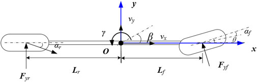
FIGURE 2. 2 DOF reference model.

The 2 DOF model can be built based on the simplification of Eqs 2, 4. The simplified equations to describe the lateral and yaw motion of the vehicle are Eqs 15, 16:

$m\left({\dot{v}}_y+v_x{\gamma }_r\right)=F_{yf}\cos \theta +F_{yr}(15)$

$I_z\dot{\gamma }=F_{yf}\cos \theta L_f-F_{yr}{L}_r(16)$

The relationship between the lateral force and tire sideslip angle is nonlinear. A nonlinear tire model is necessary to calculate the lateral force. A brush tire model variant of the Fiala nonlinear brush model, assuming one coefficient of friction and parabolic force distribution, as described by Pacejka (Pacejka, 2012). In the brush model, the lateral force, $F_{yi}$, can be expressed as:

$F_{yi}=\frac{C_{\alpha i}f\left({\xi }_i\right)\tan {\alpha }_i}{{\xi }_i\left(1+{\lambda }_i\right)}(17)$

$f\left({\xi }_i\right)=\{\begin{array}{c}\begin{array}{cc}{\xi }_i-\frac{{\xi }_i^2}{3\mu F_{zi}}+\frac{{\xi }_i^3}{27{\mu }^2{F}_{zi}^2}& \left|{\xi }_i\right|<3\mu F_{zi}\end{array}\\ \begin{array}{cc}\mu F_{zi}\begin{array}{ccc}\begin{array}{cc}\begin{array}{cc}& \end{array}& \end{array}& & \end{array}& \left|{\xi }_i\right|\ge 3\mu F_{zi}\end{array}\end{array}(18)$

${\xi }_i=\sqrt{C_{xi}^2{\left(\frac{{\lambda }_i}{1+{\lambda }_i}\right)}^2+C_{\alpha i}^2{\left(\frac{\tan {\alpha }_i}{1+{\lambda }_i}\right)}^2}(19)$

${\lambda }_i=\frac{R_{\omega }{\omega }_i-v_x}{\max \left(R_{\omega }{\omega }_i,v_x\right)}(20)$

The footnote, $i$, stands front $f$ and rear $r$, respectively. The normal force of the front and rear axle, $F_{zf}$ and $F_{zr}$, can be defined as:

$\{\begin{array}{c}{F}_{zf}=\frac{mg{L}_r}{\left(L_f+L_r\right)}\\ F_{zr}=\frac{mg{L}_f}{\left(L_f+L_r\right)}\end{array}(21)$

${\alpha }_{sl}$ is the sideslip angle corresponding to the full saturation of the tire force.

${\alpha }_{sl}=\arctan \frac{3\mu F_z}{C_{\alpha }}(22)$

${\alpha }_f$ and ${\alpha }_r$ are the sideslip angle of the front and rear tires, respectively.

$\{\begin{array}{c}{\alpha }_f=\frac{v_y+L_f\gamma }{v_x}\\ {\alpha }_r=\frac{v_y-L_r\gamma }{v_x}\end{array}(23)$

Model validation

To investigate the vehicle dynamics control algorithm, the accuracy and efficiency of the model should be taken into consideration. The model should be able to reflect the vehicle dynamics but not too complicated. Normally, the vehicle field test result or results are simulated by commercial platforms, such as Adams/Car and Carsim. In this case, Carsim is chosen to validate the established model.

The severe double lane-change maneuver is one of the most common conditions to verify the accuracy of models. It is a dynamic process consisting of rapidly driving a car from its original lane to another parallel lane and returning to the initial lane. During the process, the vehicle should not exceed the lane boundaries. It is widely used in vehicle stability assessment because its result is repeatable and discriminatory. In this case, the double lane-change maneuver on the high adhesion road with the speed of 80 km/h is chosen to verify the established models.

The vehicle yaw rate, sideslip angle, and trajectory of the established models and Carsim model in the double-lane change condition on the road with the adhesion of 0.3 are compared in Figures 3–5.

FIGURE 3

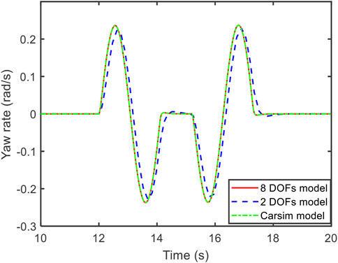
FIGURE 3. Comparison of yaw rate.

FIGURE 4

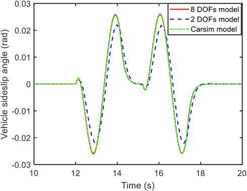
FIGURE 4. Comparison of vehicle sideslip angle.

FIGURE 5

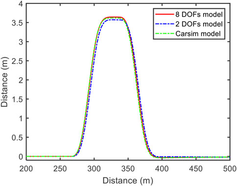
FIGURE 5. Comparison of vehicle trajectory.

According to the comparison in Figures 3–5, the output of the established 8 DOFs and 2 DOFs models is close to the Carsim. Taking the result of Carsim as the baseline, the MAPE (mean absolute percentage error) is listed in Table 2.

TABLE 2

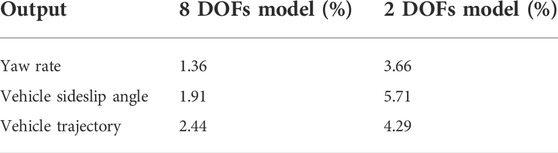
TABLE 2. MAPE of the established models.

The MAPE of the 8 DOFs model is lower than the 2DOFs model. The MAPE of the 2 DOFs model stays at a relatively low level, the maximum MAPE is lower than 6%. Therefore, these two models can be used in further analysis.

Design of control system

The structure of the proposed control strategy is shown in Figure 6. The reference model is a 2 DOF model with a nonlinear brush tire. The main goal of the control system is to make the actual yaw rate, $\gamma$, to follow the ideal yaw rate, ${\gamma }_r$, generated by the reference model and maintain the vehicle sideslip angle, $\beta$, in a certain range to prevent the vehicle from spinning. According to the comparison of the ideal and actual yaw rate and vehicle sideslip angle, the controller generates the active steering angle, $\mathrm{\Delta }\theta$, and yaw moment, $\mathrm{\Delta }{M}_z$. The yaw moment is converted to driving torque on the four wheel motors.

FIGURE 6

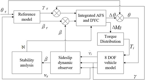
FIGURE 6. Structure of control strategy.

Integrated AFS and DYC controller

Based on Eqs 14–17, the state-space function of the 2 DOF model can be expressed as:

$\dot{x}\left(t\right)=\mathrm{A}x\left(t\right)+{\mathrm{B}}_{1}y\left(t\right)+{\mathrm{B}}_{2}u\left(t\right)(24)$

$x\left(t\right)={\left[\begin{array}{cc}{\beta }_r& {\gamma }_r\end{array}\right]}^T(25)$

${\rm A}=[\begin{array}{cc}\frac{2(k_f+k_r)}{m{v}_x}& -1+\frac{2(L_r{k}_r-L_f{k}_f)}{m{v}_x^2}\\ \frac{2(L_r{k}_r-L_f{k}_f)}{I_z}& \frac{2{\left(L_f^2{k}_f+L_r^{2}k\right)}_r}{v_x}\end{array}](26)$

${\mathrm{B}}_1={\left[\begin{array}{cc}-\frac{2k_f}{m{v}_x}& -\frac{2L_f{k}_f}{I_z}\end{array}\right]}^T(27)$

$y\left(t\right)=\theta (28)$

${\mathrm{B}}_2=\left[\begin{array}{cc}\frac{2k_f}{m{v}_x}& 0\\ \frac{2L_f{k}_f}{I_z}& \frac{1}{I_z}\end{array}\right](29)$

$u\left(t\right)={\left[\begin{array}{cc}\mathrm{\Delta }\theta & \mathrm{\Delta }{M}_z\end{array}\right]}^T(30)$

The lateral stiffness of the front tire can be gained based on Eqs 16, 22.

$\{\begin{array}{c}{k}_f=\frac{F_{yf}}{{\alpha }_f}\\ k_r=\frac{F_{yr}}{{\alpha }_r}\end{array}(31)$

According to the 2 DOFs model, the ideal vehicle yaw rate and sideslip angle can be gained. The active steering angle and torque are acquired according to the optimal solution of equation (24). It can be expressed as:

$J={\displaystyle \underset{0}{\overset{\infty }{\int }}\left[x{\left(t\right)}^{T}Qx\left(t\right)+u{\left(t\right)}^{T}Ru\left(t\right)\right]}dt(32)$

Where, matrix $Q$ and $R$ are symmetric positive definite weighting matrix. The optimal controller $u\left(t\right)$ can be written as:

$u\left(t\right)=-R^{-1}{B}^{T}Px\left(t\right)=-Kx\left(t\right)(33)$

The matrix meets the Riccati equation.

$PA+A^{T}P-PB{R}^{-1}{B}^{T}P+Q=0(34)$

Coordination of AFS and DYC

Once the steering angle and yaw moment are gained, the control task should be determined. According to Aouadj’s work, the steering angle will always be taken as the input, the yaw moment will be initiated only when the vehicle is in a dangerous condition (Aouadj et al., 2020). In this case, the $\dot{\beta }-\beta$ phase portrait is used to determine the stability state of the vehicle, as shown in Figure 7.

FIGURE 7

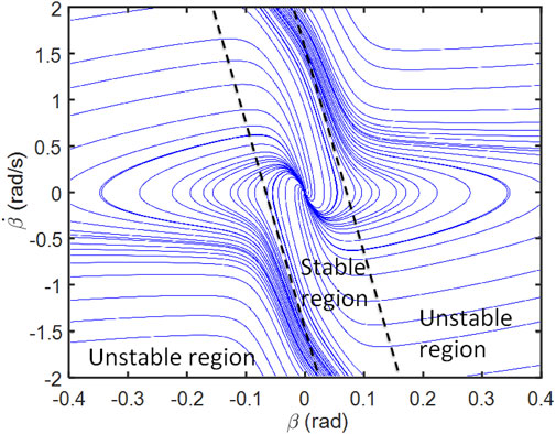
FIGURE 7. Stable region in the sideslip angle and angular velocity phase portrait.

As shown in Figure 7, the phase portrait is divided into three parts, one stable region, and two unstable regions. The boundary of the stable and stable region can be described by Eq. 35 (He et al., 2006):

$\aleph =\left|a\dot{\beta }+b\beta \right|,\aleph <1(35)$

The parameter $a$ and $b$ are acquired based on the $\dot{\beta }-\beta$ phase portrait boundary (dash lines in Figure 4).

$\dot{\beta }=\frac{a_y}{v_x}-\gamma (36)$

Simulation and discussion

There are some classical work conditions to access the vehicle’s lateral stability, such as steady steering, snake steering, fishhook, and double lane change. Among them, the double lane-change and fishhook are the most critical conditions. Therefore, they are chosen to compare the lateral stability performance with two different torque control algorithms. The double lane-change is initiated based on the regulation in ISO-3888-1–2018 (ANSI, 2018)(Passenger cars-Test track for a severe lane-change maneuver: Part 1 double-lane change), the fishhook test is based on Laboratory test procedure for dynamic rollover, the fishhook maneuver test procedure (New car assessment program, NCAP).

Double lane-change

Normally, the recommended speed on the snow or ice road is within 30 km/h. However, some drivers run the vehicle at a higher speed based on their experience. Therefore, the speed of 36 km/h is chosen to initiate the simulation.

The steering angle and torque of each wheel are shown in Figures 8–10, respectively.

FIGURE 8

FIGURE 8. Comparison of steering angle.

FIGURE 9

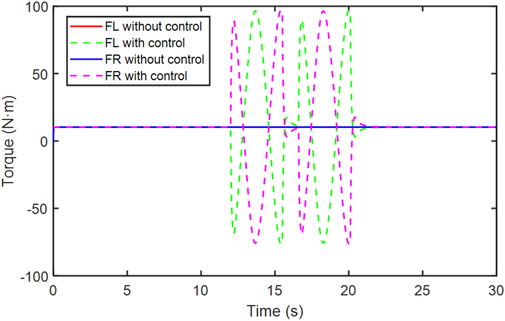
FIGURE 9. Comparison of front wheel torque.

FIGURE 10

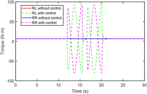
FIGURE 10. Comparison of rear wheel torque.

In Figure 8, the steering angle with and without control is compared. Without control, the steering angle is the same as the reference. With the controller, the steering angle is different from the reference, the maximum gap is 0.002 rad.

According to the comparison in Figures 9, 10, with the control algorithm, the torque varies to maintain the stability of the vehicle. The left and right wheel torque of the same axle have the opposite variation trend.

The vehicle routine, phase portrait, and yaw rate are calculated and compared in Figures 11–13.

FIGURE 11

FIGURE 11. Comparison of double lane-change routine.

FIGURE 12

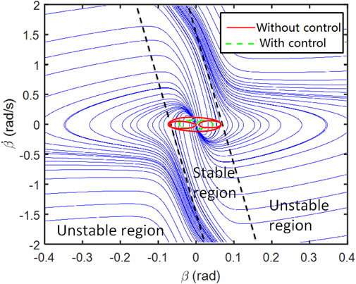
FIGURE 12. Comparison of the phase portrait.

FIGURE 13

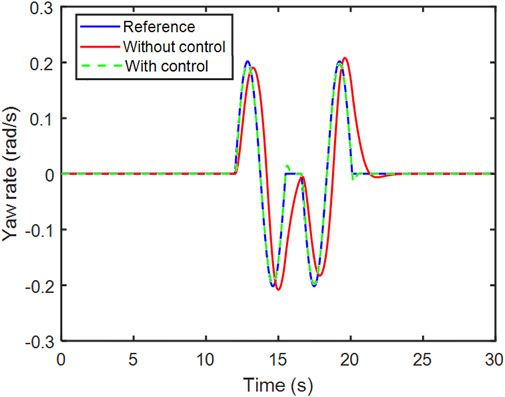
FIGURE 13. Comparison of yaw rate.

In Figure 11, the red line represents the lane boundary regulated in ISO 3888:2018. The box means the vehicle, the blue and green dash line is the vehicle routine without and with the control method. Without control, the vehicle fails to pass the double lane-change test. The maximum offset distance is 1.41 m. With the control algorithm, the vehicle can finish the test without exceeding the boundaries.

In Figure 12, it is clear that the envelope with control is smaller than the envelope without control. The envelope without exceeds the stable boundaries a bit, which means the vehicle is at the edge of stable and unstable. With the controller, both of the vehicle sideslip angle and angular velocity are maintained in a lower range.

Figure 13 shows the yaw rate variation of the reference model, without and with control. With control, the maximum error of the reference model is 0.01 rad/s. Without control, the actual vehicle yaw rate is lag behind the reference model with approximately 0.5 s, the maximum error is 0.1 rad/s if the effect of the time delay is eliminated.

Fishhook maneuver

Fishhook maneuver is the test procedure of the New Car Assessment Program (NCAP) used by the National Highway Traffic Safety Administration (NHSTA) to evaluate light vehicle dynamic rollover maneuver. This test procedure is also used by the researchers to evaluate the lateral stability (Jin et al., 2017). According to the test procedure, the steering angle variation during the process is shown in Figure 14 (without control).

FIGURE 14

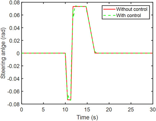
FIGURE 14. Steering angle variation during the fishhook maneuver.

With the controller, the AFS makes the steering angle varies from the reference angle. The gap occurs at the sudden change of the steering angle, the maximum gap is 0.016 rad.

During the fishhook maneuver, the toque of the wheels is shown in Figures 15, 16.

FIGURE 15

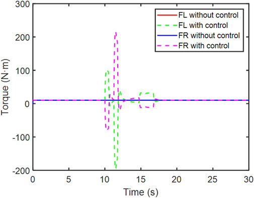
FIGURE 15. Comparison of front wheel torque.

FIGURE 16

FIGURE 16. Comparison of rear wheel torque.

The vehicle routine, phase portrait, and yaw rate during the fishhook maneuver are calculated and compared in Figures 17–19.

FIGURE 17

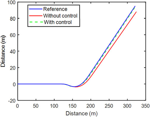
FIGURE 17. Comparison of double lane-change routine.

FIGURE 18

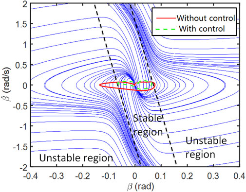
FIGURE 18. Comparison of the phase portrait.

FIGURE 19

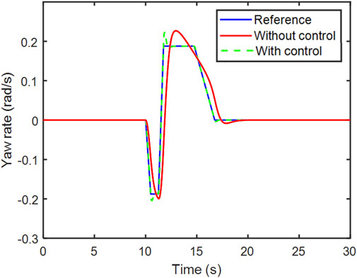
FIGURE 19. Comparison of yaw rate.

Figure 17 illustrates the vehicle track of the reference model, with and without the control algorithm. With the integrated control, the gap between the reference model and the 8 DOF model is relatively small. The difference between the track of the model without control and the reference model occurs at the beginning of the steering and gets bigger with time.

Figure 18 demonstrates the difference of the phase portrait track. The track of the model without control exceeds the boundary of stable boundaries. The variation range of the vehicle sideslip angle is much higher than the vehicle sideslip angular velocity. With the help of control method, the AFS and DYC are coordinated and the track stays in the stable region.

In Figure 19, the yaw rate of the three models is compared. The yaw rate of the reference model varies strictly with the steering input. The yaw rate of the model with control is close to the yaw rate of the reference model, except for the two inflection points 10.5 and 11.75 s, the error between the model with control and reference model gets bigger. The maximum error is 0.03 rad/s. For the yaw rate of the model without control, it takes more time to eliminate the gap to the reference model, the maximum error is 0.03 rad/s. However, the mean error is bigger than the model with control.

Conclusion

The goal of this study is to design an integrated vehicle dynamics controller to enhance the vehicle lateral stability. To deal with the critical condition on a low adhesion coefficient road, a 2 DOF nonlinear reference model and 8 DOFs model are built and validated by Carsim. The integrated AFS and DYC controller is designed. Based on the dynamic analysis, the effectiveness of the provided algorithm in two typical conditions is proved by the 8 DOFs model.

Without the control method, the vehicle fails to pass the double lane-change test at the speed of 36 km/h on the road with a low adhesion coefficient of 0.3. The track on the $\dot{\beta }-\beta$ phase portrait exceeds the stable region in both the double lane-change and fishhook maneuvers. With the integrated controller, the vehicle yaw rate, the routine can follow the reference model with a much smaller error, and the track on the $\dot{\beta }-\beta$ phase portrait stays in the stable region, which means the vehicle stability is enhanced.

According to the comparison of lateral stability indicators of double lane-change and fishhook maneuver, the goal is achieved, the lateral stability and path tracking ability of the vehicle on the low adhesion road is improved. The improvement of the vehicle safety and path tracking ability lays a good foundation for the whole vehicle-to-grid system.

Data availability statement

The raw data supporting the conclusion of this article will be made available by the authors, without undue reservation.

Author contributions

YW is responisble for the simulation and writting of this paper. YL provides the assistance of the simulation and vehicle parameters. PW provides the original idea and funding.

Funding

This study was funded by the Innovative Research Team Development Program of Ministry of Education of China (IRT_17R83), and the 111 Project (B17034) of China.

Conflict of interest

The authors declare that the research was conducted in the absence of any commercial or financial relationships that could be construed as a potential conflict of interest.

Publisher’s note

All claims expressed in this article are solely those of the authors and do not necessarily represent those of their affiliated organizations, or those of the publisher, the editors and the reviewers. Any product that may be evaluated in this article, or claim that may be made by its manufacturer, is not guaranteed or endorsed by the publisher.

References

Adam, A. A. (2013). Accurate modeling of PMSM for differential mode current and differential torque calculation.” in International Conference on Computing, Khartoum, August 26, 2009. IEEE.

CrossRef Full Text | Google Scholar

ANSI (2018). Passenger cars-test track for a severe lane-change maneuver: obstacle avoidance-Part 1: Double lane-change. ISO 3888-1:2018 (E).

Google Scholar

Aouadj, N., Hartani, K., and Fatiha, M. (2020). New integrated vehicle dynamics control system based on the coordination of active front steering, direct yaw control, and electric differential for improvements in vehicle handling and stability. SAE Int. J. Veh. Dyn. Stab. NVH 4, 119–133. doi:10.4271/10-04-02-0009

CrossRef Full Text | Google Scholar

Boada, B. L., Boada, M. J. L., and Díaz, V. (2005). Fuzzy-logic applied to yaw moment control for vehicle stability. Veh. Syst. Dyn. 43 (10), 753–770. doi:10.1080/00423110500128984

CrossRef Full Text | Google Scholar

Bobier, C. G., and Gerdes, J. C. (2013). Staying within the nullcline boundary for vehicle envelope control using a sliding surface. Veh. Syst. Dyn. 51 (2), 199–217. doi:10.1080/00423114.2012.720377

CrossRef Full Text | Google Scholar

Chen, T., Xu, X., Li, Y., Wang, W., and Chen, L. (2017). Speed-dependent coordinated control of differential and assisted steering for in-wheel motor driven electric vehicles. Proceedings of the Institution of Mechanical Engineers Part D Journal of Automobile Engineering.095440701772818

Google Scholar

Dai, Y., Yu, L., Song, J., and Zhao, W. (2019). The differential braking steering control of special purpose flat-bed electric vehicle. Detroit: WCX SAE World Congress Experience.

Google Scholar

Goodarzi, A., Soltani, A., and Esmailzadeh, E. (2011). Active variable wheelbase as an innovative approach in vehicle dynamic control.” in ASME 2011 International Design Engineering Technical Conferences and Computers and Information in Engineering Conference, Khartoum, August 26, 2009.

CrossRef Full Text | Google Scholar

He, J., Crolla, D. A., Levesley, M. C., and Manning, W. J. (2006). Coordination of active steering, driveline, and braking for integrated vehicle dynamics control. Proc. Institution Mech. Eng. Part D J. Automob. Eng. 220 (D10), 1401–1420. doi:10.1243/09544070jauto265

CrossRef Full Text | Google Scholar

Inagaki, S., Kushiro, I., and Yamamoto, M. (1994). Analysis on vehicle stability in critical cornering using phase-plane method. JSAE Rev. 16 (21), 216.

Google Scholar

Jaafari, S., and Shirazi, K. H. (2016). A comparison on optimal torque vectoring strategies in overall performance enhancement of a passenger car. Proc. Institution Mech. Eng. Part K J. Multi-body Dyn. 1464419315627113, 469–488. doi:10.1177/1464419315627113

CrossRef Full Text | Google Scholar

Jin, X., Yu, Z., Yin, G., and Wang, J. (2017). Improving vehicle handling stability based on combined afs and dyc system via robust takagi-sugeno fuzzy control. IEEE Trans. Intell. Transp. Syst. 19, 2696–2707. doi:10.1109/tits.2017.2754140

CrossRef Full Text | Google Scholar

Khalfaoui, M., Hartani, K., Merah, A., and Aouadj, N. (2018). Development of shared steering torque system of electric vehicles in presence of driver behaviour estimation. Int. J. Veh. Aut. Syst. 14 (1), 18. doi:10.1504/ijvas.2018.093100

CrossRef Full Text | Google Scholar

Li, S., Zhao, J., Yang, S., and Fan, H. (2019). Research on a coordinated cornering brake control of three-axle heavy vehicles based on hardware-in-loop test. IET Intell. Transp. Syst. 13 (5), 905–914. doi:10.1049/iet-its.2018.5406

CrossRef Full Text | Google Scholar

Liu, Z., Pei, X., Chen, Z., Yang, B., and Guo, X. (2019). Differential speed steering control for four-wheel distributed electric vehicle. Detroit: WCX SAE World Congress Experience.

Google Scholar

Ono, E., Hosoe, S., Tuan, H. D., and Doi, S. (1998). Bifurcation in vehicle dynamics and robust front wheel steering control. IEEE Trans. Control Syst. Technol. 6 (3), 412–420. doi:10.1109/87.668041

CrossRef Full Text | Google Scholar

Pacejka, H. B., and Besselink, I. J. M. (1997). Magic Formula tyre model with transient properties. Veh. Syst. Dyn. 27 (S1), 234–249. doi:10.1080/00423119708969658

CrossRef Full Text | Google Scholar

Pacejka, H. B. (2012). Tire and vehicle dynamics. Third Edition. Oxford. xiii-xvi.

Google Scholar

Soares, N., Martins, A. G., Carvalho, A. L., Caldeira, C., Du, C., Castanheira, E., et al. (2018). The challenging paradigm of interrelated energy systems towards a more sustainable future. Renew. Sustain. Energy Rev. 95 (NOV), 171–193. doi:10.1016/j.rser.2018.07.023

CrossRef Full Text | Google Scholar

Truong, T., Tomaske, V., and Winfried, D. (2013). Active front steering system using adaptive sliding mode control.” in Chinese control and decision conference, Khartoum, August 26, 2009.

Google Scholar

Xu, K., Luo, Y., Yang, Y., and Xu, G. (2019). Review on state perception and control for distributed drive electric vehicles. J. Mech. Eng. 55 (22), 60. doi:10.3901/JME.2019.22.060

CrossRef Full Text | Google Scholar

Zhang, L., and Wu, G. (2016). Combination of front steering and differential braking control for the path tracking of autonomous vehicle. WCX SAE World Congress Experience.

Google Scholar

Zheng, H., Wang, L., and Zhang, J. (2018). Comparison of active front wheel steering and differential braking for yaw/roll stability enhancement of a coach. SAE Int. J. Veh. Dyn. Stab. NVH 2 (4)–283. doi:10.4271/2018-01-0820

CrossRef Full Text | Google Scholar