A Convex–Concave Procedure-Based Method for Optimal Power Flow of Offshore Wind Farms

In recent years, offshore wind farms have boomed all over the world. It is essential to manage the energy dispatch of the offshore wind power systems to reduce transmission losses. This article proposes an optimization method for the optimal power flow of offshore wind power systems based on the convex–concave procedure. First, the nonlinear variables in the power flow constraints of the offshore wind power system are relaxed with newly defined variables. Second, the non-convex constraints are reconstructed according to the variables’ characteristics so that the optimization method satisfies all constraints at the same time. Meanwhile, by applying the Taylor series expansion, the relaxation variables’ gaps are changed dynamically, and the convex relaxation is tightened to ensure the effectiveness of the proposed method. Finally, the feasibility of the relaxation and the optimized solution is verified by the simulation to realize the power optimization in the real offshore wind system.

1 Introduction

With the steady progress of energy reforms around the world, the proportion of renewable energy sources, such as wind energy and solar energy, is increasing (Zhang et al., 2017). It is estimated that by 2035, the installed capacity of wind power will reach more than one billion kilowatts, of which the offshore wind power is about 350 million kilowatts. Wind power will become one of the main power sources affecting each country’s energy structure and security. At the same time, considering the vigorous development trend of offshore oil and gas platforms, and their complex network format, it is very significant to carry out energy management for offshore wind power systems (Shafiee, 2015).

In energy management, how to reduce system losses is the top priority of optimization (Khan et al., 2016; Li Z. et al., 2020). The loss of offshore wind power is usually caused by line losses of the submarine transmission cable (Apostolaki-Iosifidou et al., 2019). Therefore, it is of great significance to propose an effective solution method to reduce the line losses on the basis of ensuring energy conservation and satisfying the corresponding physical relationship on the basis of how to carry out refined physical modelling for offshore wind power systems.

The offshore wind system is a typical nonlinear system. In the optimization of nonlinear systems, since the problem is non-convex and NP (HardKonar and Sidiropoulos, 2017), the commonly used solution methods are the linear programming method based on the approximate fitting (Bourguignon et al., 2015), gradient (Guirguis et al., 2016; Neftci et al., 2019) and Newton method-based algorithm (Li et al., 2020a), Lagrange multiplier method (Ruan et al., 2020; Xie et al., 2022), interior point method (Fazlyab et al., 2017), and various heuristic and intelligent algorithms (Rokbani et al., 2021; Goli et al., 2021; Li et al., 2022). In these algorithms, the approximated method has high solving efficiency, but it will lead to some errors in the process of linearization, which affects the feasibility of the optimal solution. Gradient and Newton-based algorithms require a high-quality initial value in the iterative calculation and may fall into the ill condition. Lagrange multiplier and interior point method have certain requirements for the value of obstacle function. Therefore, it is difficult to solve the nonlinear and non-convex problem using the common analytical solution algorithm. When using the heuristic algorithm, it needs a lot of running time and storage space, and it is hard to find the global optimal solution.

In order to find the global optimal solution of the optimization problem, the convex optimization-based methods have gradually entered the field of power system management. This is because if an optimization problem can be written in a standard convex optimization format, the local optimal solution is the global one. In addition, convex optimization can be solved efficiently by many analytical methods (Boyd et al., 2004). Therefore, to apply the convex optimization technique into non-convex and nonlinear problems, some relaxation methods should be imposed to reshape the non-convex solution domain.

According to the mathematical expression form of the relaxation, the convex relaxation methods can be roughly divided into second-order cone relaxations (Abdelouadoud et al., 2015), semi-definite relaxations (Jubril et al., 2014), convex hull relaxations (Li Q et al., 2018), and quadratic relaxations (Hijazi et al., 2017). Among these methods, the method proposed by Li Y et al. (2018) showed that the second-order cone relaxation method is suitable for the network with a radial topology, of which the recovery of the angle information is conditional. Ma et al. (2020) pointed out that semi-definite programming cannot obtain the feasible optimal solution in a special three-node network. Cremers and Kolev (2010) pointed out that the constructions of convex hulls lead to different relaxed regions in the solution domain. Chen et al. (2021) proposed a quadratic relaxation with certain constraints on the angle difference in the network, which can only be applied to the special meshed topology. Therefore, the above methods have some limitations in the application of power optimization, and it is difficult to ensure the accuracy of relaxation.

In the current research on the energy optimization of offshore wind farms, few methods use convex relaxations. The convex relaxation-based methods will enlarge the solution domain through the variable replacement, which may cause the loss of information. Therefore, it is challenging to recover the complete system information after relaxations, and the feasible optimal solution cannot be obtained unless the conditions of exact relaxations are met. The change of topology and system parameters will result in inexact relaxations. So the generality and flexibility of the convex relaxation-based method is poor.

In summary, how to use the convex relaxation method to realize the accurate relaxation is of great significance. To fill the research gap of the above literature, this article proposes a convex–concave procedure-based method for the energy optimization of offshore wind power systems. This method mainly focuses on the problem of wind turbines’ output and the energy distribution in the offshore wind power system. This method inherits the advantages of traditional convex optimization methods, which can be efficiently solved with the global optimal solution. In this method, the optimization problem of the offshore wind power system is first modelled mathematically, and the second-order cone relaxation method is used to deal with the non-convex constraints in the optimization. Then, in order to reduce the relaxation gap, a Taylor series expansion-based technique is imposed to contract the relaxation region; that is, the iterative process is imposed with the convex–concave procedure so that the solution domain is close to the one before relaxation. Thus, the efficient energy management of offshore wind power systems can be achieved, and the energy management problem of the offshore wind power system can be solved while maximizing the economic benefits of the system.

2 Optimization Model

Figure 1 is a schematic diagram of offshore wind power systems. Among them, the wind power system is usually composed of offshore wind farms and electrical collector systems, which interconnects multiple wind farms. In order to transfer the power of the offshore wind power system to the power grid side, the substation is required.

FIGURE 1

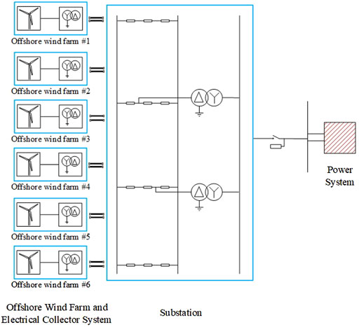
FIGURE 1. Schematic diagram of offshore wind power systems.

The research of this article focuses on the offshore wind power system, that is, the energy management of the offshore wind farms and collector line systems. The offshore wind power system is a typical nonlinear system, of which the mathematical model is non-convex. It is composed of the objective function, equality constraints, and inequality constraints. The aim of the optimization is to maximize the transmitted power to the grid. The constraints are about the power flow, energy, voltage, load, and generators’ constraints. In addition, the topology of the system should be considered as well.

In the optimization model of the offshore wind system, define the voltage variable of each node i with the complex variable U_i = V_i∠θ_i. The generated active and reactive power of node i is $P_i^g$ and $Q_i^g$. The active and reactive consumption power of node i is $P_i^c$ and $Q_i^c$. For branch i ∼ j, the current variable is I_ij, the admittance is Y_ij, the conductance is G_ij, and the susceptance is B_ij. The transmitted apparent power, active power, and reactive power of the branch i ∼ j are denoted as S_ij, P_ij, and Q_ij, respectively.

2.1 Objective Function

The objective function of the offshore wind farm is to maximize the on-grid electricity, that is, to minimize the transmission loss of the system. The mathematical expression of the power loss is

$f=\sum \underset{i}{\overset{g}{P}}-\sum \underset{i}{\overset{c}{P}}.(1)$

$P_i^g$ and $P_i^c$ are the generated power and consumption power of node i, respectively.

2.2 System Constraints

Based on the operating conditions and physical relationships of the offshore wind power system, the constraints are established as follows:

1) The relationship between the transmitted power and current with the node’s voltage is

$S_{ij}=U_i{I}_{ij}^{*}.(2)$

In the abovementioned equation,^* is the conjugate operator. Variables S_ij, U_i, and I_ij are complex variables.

2) The relationship between node’s voltage and branch current:

$I_{ij}=\left(U_i-U_j\right)Y_{ij}.(3)$

where Y_ij is the complex variable.

3) Power balance law of active and reactive power:

$P_i=\sum P_{ij}=\sum \underset{i}{\overset{g}{P}}-\underset{i}{\overset{c}{P}}.(4)$

$Q_i=\sum Q_{ij}=\sum \underset{i}{\overset{g}{Q}}-\underset{i}{\overset{c}{Q}}.(5)$

Superscripts g and c denote the generator nodes and load nodes, respectively. In the offshore wind farm system, a majority of the nodes are generator nodes.

4) Voltage ranges

$V_i^{\min }\le V_i\le V_i^{\max }.(6)$

${\theta }_i^{\min }\le {\theta }_i\le {\theta }_i^{\max }.(7)$

5) Power ranges

$P_i^{c\min }\le P_i^c\le P_i^{c\max }.(8)$

$Q_i^{c\min }\le Q_i^c\le Q_i^{c\max }.(9)$

$P_i^{g\min }\le P_i^g\le P_i^{g\max }.(10)$

$Q_i^{g\min }\le Q_i^g\le Q_i^{g\max }.(11)$

Superscripts min and max are the lower and upper bounds, which are constants. For the active power and reactive power of node i, the limited bounds are defined according to the operating constraints of the equipment. The active power and reactive power in the abovementioned formula are real variables.

6) Branch constraints:

$P_{ij}^{\min }\le P_{ij}\le P_{ij}^{\max }.(12)$

$Q_{ij}^{\min }\le Q_{ij}\le Q_{ij}^{\max }.(13)$

For the active power and reactive power of the transmission line, according to the operating constraints of lines, the bounds are limited.

2.3 Optimization Model

Based on the objective function and constraints modelled earlier, the optimization model can be summarized as

$\begin{array}{ll}\hfill & \min (1)\hfill \\ \hfill & \text{s.t.}(2)-(13).\hfill \end{array}(14)$

In this optimization problem, because of the constraints in Eqs 2, 3, it is a non-convex, nonlinear, and NP-hard problem.

By adjusting the active and reactive power output of the offshore wind power system, it can provide reactive power support for the offshore collector systems. Thus, the power loss and the reactive power configuration of the substations can be reduced. In view of this, the article proposes a convex relaxation method to optimize the offshore wind power system efficiently.

3 Convex Relaxation-Based Method for Offshore Wind Systems

3.1 Slack Variables’ Definition

Six real variables are defined as follows:

$a_i=V_i^2\cos {\theta }_i^2,(15)$

$b_i=V_i^2\sin {\theta }_i^2,(16)$

$a_{ij}=V_i\cos {\theta }_i{V}_j\cos {\theta }_j,(17)$

$b_{ij}=V_i\sin {\theta }_i{V}_j\sin {\theta }_j,(18)$

$s_{ji}=V_{j}cos{\theta }_j{V}_i\sin {\theta }_i,(19)$

$s_{ij}=V_i\cos {\theta }_i{V}_j\sin {\theta }_j.(20)$

By substituting Eq. 3 into Eq. 2, we can get the branch power flow of active power and reactive power as

$P_{ij}=\mathfrak{R}\left(V_i{V}_i^{*}{Y}_{ij}^{*}\right)-\mathfrak{R}\left(V_i{V}_j^{*}{Y}_{ij}^{*}\right),(21)$

$Q_{ij}=\mathfrak{I}\left(V_i{V}_i^{*}{Y}_{ij}^{*}\right)-\mathfrak{I}\left(V_i{V}_j^{*}{Y}_{ij}^{*}\right),(22)$

where $\mathfrak{R}$ and $\mathfrak{I}$ represent the real and imaginary parts of the complex variables, respectively. By replacing the voltage-related variables with the newly defined variables, the branch power flow of each transmission line from the two directions will become

$P_{ij}=-\left(a_{ij}+b_{ij}\right)G_{ij}+B_{ij}\left(s_{ji}-s_{ij}\right)+G_{ij}\left(a_i+b_i\right)(23)$

$P_{ji}=-\left(a_{ij}+b_{ij}\right)G_{ij}-B_{ij}\left(s_{ji}-s_{ij}\right)+G_{ij}\left(a_j+b_j\right)(24)$

$Q_{ij}=-\left(a_{ij}+b_{ij}\right)B_{ij}-G_{ij}\left(s_{ji}-s_{ij}\right)+B_{ij}\left(a_i+b_i\right)(25)$

$Q_{ji}=-\left(a_{ij}+b_{ij}\right)B_{ij}+G_{ij}\left(s_{ji}-s_{ij}\right)+B_{ij}\left(a_j+b_j\right)(26)$

Since we have the voltage constraints in Eq. 6 and Eq. 7, the newly defined six variables have the corresponding ranges as well.

${\left(V_i^{\min }\right)}^2\le a_i+b_i\le {\left(V_i^{\max }\right)}^2(27)$

$\min \left\{V_i{V}_{j}cos\left({\theta }_{ij}\right)\right\}\le a_{ij}+b_{ij}\le \max \left\{V_i{V}_{j}cos\left({\theta }_{ij}\right)\right\},(28)$

$\min \left\{sin\left({\theta }_{ij}\right)\right\}\le s_{ji}-s_{ij}\le \max \left\{sin\left({\theta }_{ij}\right)\right\},(29)$

where ${\theta }_{ij}\in [{\theta }_{ij}^{\min },{\theta }_{ij}^{\max }]$. The limits of θ_ij can be obtained from the ranges of θ_i and θ_j. Therefore, min{ cos(θ_ij)}, max{ cos(θ_ij)}, min{ sin(θ_ij)}, and max{ sin(θ_ij)} are known in advance according to the relationship of trigonometric functions. The six variables defined in Eqs 15–20 have the following four series of equality constraints.

$s_{ij}^2=a_i{b}_j(30)$

$s_{ji}^2=a_j{b}_i(31)$

$a_{ij}^2=a_i{a}_j(32)$

$b_{ij}^2=b_i{b}_j(33)$

With the slack variables added, the optimization problem in Eq. 14 can be rewritten as

$\begin{array}{ll}\hfill & \min (1)\hfill \\ \hfill & \text{s.t.}(4)-(5),(8)-(13),(23)-(33).\hfill \end{array}(34)$

The non-convexity of Eq. 34 comes from the constraints of Eqs 30–33, which are in standard quadratic formats. To deal with this non-convexity, the convex–concave procedure is imposed in the next subsection.

3.2 Convex–Concave Procedure

For the constraints in Eqs 30–33, we can reconstruct them with the two groups of inequality constraints as

$\frac{{\left(a_i+a_j\right)}^2}{4}-\left[a_{ij}^2+\frac{{\left(a_i-a_j\right)}^2}{4}\right]\le 0,(35)$

$\frac{{\left(b_i+b_j\right)}^2}{4}-\left[b_{ij}^2+\frac{{\left(b_i-b_j\right)}^2}{4}\right]\le 0,(36)$

$\frac{{\left(a_i+b_j\right)}^2}{4}-\left[s_{ij}^2+\frac{{\left(a_i-b_j\right)}^2}{4}\right]\le 0,(37)$

$\frac{{\left(a_i+b_j\right)}^2}{4}-\left[s_{ji}^2+\frac{{\left(a_j-b_i\right)}^2}{4}\right]\le 0,(38)$

$\frac{{\left(a_i+a_j\right)}^2}{4}-\left[a_{ij}^2+\frac{{\left(a_i-a_j\right)}^2}{4}\right]\ge 0,(39)$

$\frac{{\left(b_i+b_j\right)}^2}{4}-\left[b_{ij}^2+\frac{{\left(b_i-b_j\right)}^2}{4}\right]\ge 0,(40)$

$\frac{{\left(a_i+b_j\right)}^2}{4}-\left[s_{ij}^2+\frac{{\left(a_i-b_j\right)}^2}{4}\right]\ge 0,(41)$

$\frac{{\left(a_i+b_j\right)}^2}{4}-\left[s_{ji}^2+\frac{{\left(a_j-b_i\right)}^2}{4}\right]\ge 0.(42)$

It can be found that the constraints in Eqs 39–42 are second-order cone relaxations, which are convex, and the convex optimization problem is defined as

$\begin{array}{ll}\hfill & \min (1)\hfill \\ \hfill & \text{s.t.}(4)-(5),(8)-(13),(23)-(29),(39)-(42).\hfill \end{array}(43)$

Set the convex solution domain of convex optimization Eq. 43 with the convex set Ω. In addition, all the variables in Eq. 43 are defined with the convex set X. Then Eq. 34 can be equivalently written as

$\begin{array}{ll}\hfill & \text{min}{f}_0\left(X\right),\hfill \\ \hfill & \text{s.t.}{f}_k\left(X\right)-g_k\left(X\right)\le 0.X\in \mathrm{\Omega }.\hfill \end{array}(44)$

In Eq. 44, f_k(X) refers to the first term in Eqs 35–38, and g_k(X) refers to the second term in Eqs 35–38. It can be found that both f_k(X) and g_k(X) are convex functions.

Due to the policy of first-order Taylor expansion series at X(t), where t is the index number of the iteration times, g_k(X) in Eqs 35–38 can be linearized as

$\begin{array}{ll}\hfill g_k{\left(X;X^{\left(t\right)}\right)}^{{\left(a\right)}^{\prime }}& =a_{ij}^2+\frac{{\left(a_i-a_j\right)}^2}{4}\stackrel{\mathrm{\Delta }}{=}{a}_{ij}^{2\left(t\right)}+2a_{ij}^{\left(t\right)}\left(a_{ij}-a_{ij}^{\left(t\right)}\right)\hfill \\ \hfill & +\frac{{\left(a_i^{\left(t\right)}-a_j^{\left(t\right)}\right)}^2}{4}+\frac{a_i^{\left(t\right)}-a_j^{\left(t\right)}}{2}\hfill \\ \hfill & \times \left(a_i-a_i^{\left(t\right)}-a_j+a_j^{\left(t\right)}\right)\hfill \end{array}(45)$

$\begin{array}{ll}\hfill g_k{\left(X;X^{\left(t\right)}\right)}^{{\left(b\right)}^{\prime }}& =b_{ij}^2+\frac{{\left(b_i-b_j\right)}^2}{4}\stackrel{\mathrm{\Delta }}{=}{b}_{ij}^{2\left(t\right)}+2b_{ij}^{\left(t\right)}\left(s_{ij}-b_{ij}^{\left(t\right)}\right)\hfill \\ \hfill & +\frac{{\left(b_i^{\left(t\right)}-b_j^{\left(t\right)}\right)}^2}{4}+\frac{b_i^{\left(t\right)}-b_j^{\left(t\right)}}{2}\hfill \\ \hfill & \times \left(b_i-b_i^{\left(t\right)}-b_j+b_j^{\left(t\right)}\right)\hfill \end{array}(46)$

$\begin{array}{ll}\hfill g_k{\left(X;X^{\left(t\right)}\right)}^{{\left(c\right)}^{\prime }}& =s_{ij}^2+\frac{{\left(a_i-b_j\right)}^2}{4}\stackrel{\mathrm{\Delta }}{=}{s}_{ij}^{2\left(t\right)}+2s_{ij}^{\left(t\right)}\left(s_{ij}-s_{ij}^{\left(t\right)}\right)\hfill \\ \hfill & +\frac{{\left(a_i^{\left(t\right)}-b_j^{\left(t\right)}\right)}^2}{4}+\frac{a_i^{\left(t\right)}-b_j^{\left(t\right)}}{2}\hfill \\ \hfill & \times \left(a_i-a_i^{\left(t\right)}-b_j+b_j^{\left(t\right)}\right)\hfill \end{array}(47)$

$\begin{array}{ll}\hfill g_k{\left(X;X^{\left(t\right)}\right)}^{{\left(d\right)}^{\prime }}& =s_{ji}^2+\frac{{\left(a_j-b_i\right)}^2}{4}\stackrel{\mathrm{\Delta }}{=}{s}_{ji}^{2\left(t\right)}+2s_{ji}^{\left(t\right)}\left(s_{ji}-s_{ji}^{\left(t\right)}\right)\hfill \\ \hfill & +\frac{{\left(a_j^{\left(t\right)}-b_i^{\left(t\right)}\right)}^2}{4}+\frac{a_j^{\left(t\right)}-b_i^{\left(t\right)}}{2}\hfill \\ \hfill & \times \left(a_j-a_j^{\left(t\right)}-b_i+b_i^{\left(t\right)}\right).\hfill \end{array}(48)$

To drive the Taylor expansion series be exactly equal to the equality before the expansion, the penalty term is involved. $R(X)={\tau }^{(t)}{\sum }_{k=1}^w{d}_k$ is defined, where w is the total number of constraints (35)–(38) in the system, and τ^(t) indicates the penalty factor in the tth iteration whose limit is from τ^min to τ^max. d_k is an introduced non-negative variable, which is intended to be the slack variable for constraints in Eqs 35–38. Considering the sum of d_k is ${\sum }_{k=1}^w{d}_k^{(t+1)}$, which is expected to be around zero, the solution obtained from Eq. 44 will be exactly the one from Eq. 34. Therefore, the penalty term is added into the objective function to drive d_k to be zero.

With R(X) as penalty terms in the objective function, the objective function differences between the tth and the t + 1-th iteration with R(X)^(t) − R(X)^(t+1) are recorded. Substituting $g_k{(X;X^{(t)})}^{\prime }$ to replace g_k(X), optimization Eq. 44 will be

$\begin{array}{ll}\hfill & \text{min}{f}_0\left(X\right)+\tau \sum _{k=1}^w{d}_k,\hfill \\ \hfill & \text{s.t.}{f}_k\left(X\right)-g_k{\left(X;X^{\left(t\right)}\right)}^{\prime }\le d_k,X\in \mathrm{\Omega }\hfill \\ \hfill & d_k\ge 0.k=\mathrm{1,2}\dots .,w\hfill \end{array}(49)$

Since the convex–concave procedure method is an iterative algorithm, the stopping criterion will be no more the improvement of the objective function or ${\sum }_{k=1}^w{d}_k^{(t+1)}$, which tends to be zero. Moreover, τ is set with limited constant τ^max, and a step length of 1.5 is set for τ in the iteration. Thus, the algorithm allows a low penalty on violations which in turn permits an enlarged solution region with a lower objective value. Consider a very small positive δ ≈ 0 as the stopping signal. Therefore, the total stopping criterion of the convex–concave procedure method will be all of the inequalities. Thus, ${\sum }_{k=1}^w{d}_k^{(t+1)}>\delta ,{\tau }^{(t)}<{\tau }^{\max }$ and |R(X)^(t) − R(X)^(t+1)| > δ are violated. The whole solving process is shown in Figure 2.

FIGURE 2

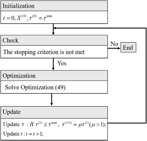
FIGURE 2. Solving process of the proposed method.

Thus, with the convex–concave procedure applied, the non-convex offshore wind system’s optimization problem in Eq. 14 is transferred to Eq. 49. In each iteration, the convex optimization is solved efficiently and the sum of gaps is considered. Thus, when the iteration is stopped, the total violations are punished and the relaxation gap will closely be zero. In summary, both the solving efficiency and the optimization precision can be guaranteed.

4 Case Study

In this article, a real offshore wind farm in China is used as the testing system. The system consists of 91 wind turbines in 14 loops. The topology is shown in Figure 3.

FIGURE 3

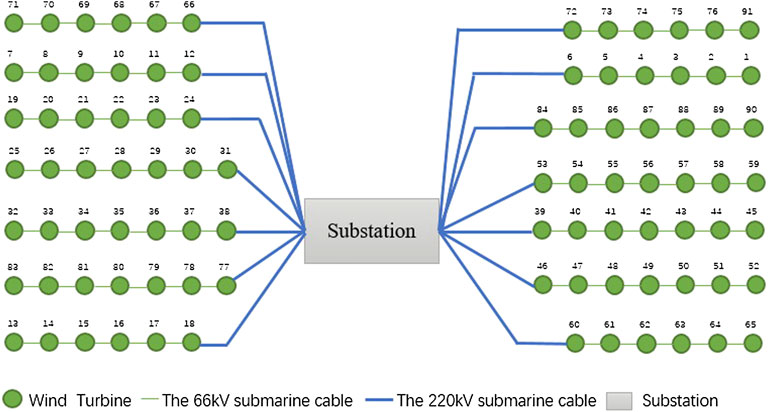
FIGURE 3. Topology of the offshore wind farm system.

In this system, the length of the submarine cable between most of the circuit is 735 m. In the circuit between No. 77 and No. 83 wind turbines and the circuit between No. 84 and No. 90 wind turbines, the length of the submarine cable is 1715 m. The selection of submarine cables between the wind turbines is decided according to the multiple factors such as the line’s current carrying capacity, thermal stability, and voltage drop. The length of the high-voltage submarine cable between the wind turbine and the offshore substation is shown in Table 1.

TABLE 1

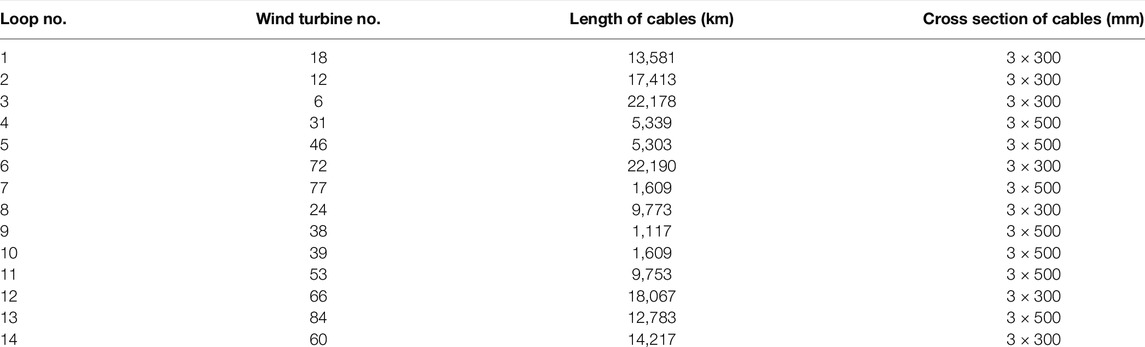
TABLE 1. Information of the connected wind turbines and their offshore submarine cables.

The relaxation model established above is built and written into Matlab through the Yalmip (Lofberg, 2004) toolbox, and solved by the IBM commercial solver CPLEX (Shinano and Fujie, 2007). The CPLEX is called to solve the convex optimization in the iterative process. In this case, the active power, reactive power, node voltage of each wind turbine node, and current and power on the lines between wind turbines are the variables to be optimized. At the same time, the upper and lower limits of the active power and reactive power of the wind turbine node, the upper and lower limits of the nodes’ voltage, and the upper and lower limits of the active power and reactive power transmission of the line are known quantities. In this optimization, the output of the active power and reactive power of the wind turbine will affect the node voltage and the current of the line connected to it, thereby affecting the line loss, resulting in the change of the on-grid power of the wind farm. If the line loss is reduced, the on-grid power will increase. Conversely, if the line loss increases, the on-grid power will decrease.

In the test, by setting the wind turbines’ output level with 25, 50, 75, and 100%, the optimized power loss is shown in Figure 4. From this, it can be found that within four times of the iterations, the objective function will no longer be changing in all scenes. In addition, in the iteration, the power loss will be smaller. That is to say, with the convex–concave procedure implemented, the objective function changes toward a better result.

FIGURE 4

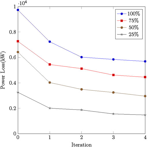
FIGURE 4. Optimization results under different wind turbine output level during iterations.

As mentioned earlier, Eq. 43 is a standard convex optimization, whose equality constraints are linear and the inequality constraints are all convex. To compare the relaxation gap of Eq. 43 and the one in Eq. 44, we have conducted the following tests when the output level of the wind turbine is 100%. The relaxation gap is defined as

$Ga{p}_{s1}=\frac{{\sum }_{ij\in E}\left(|s_{ij}^2-a_i{b}_j|\right)}{n}(50)$

$Ga{p}_{s2}=\frac{{\sum }_{ij\in E}\left(|s_{ji}^2-a_j{b}_i|\right)}{n}(51)$

$Ga{p}_a=\frac{{\sum }_{ij\in E}\left(|a_{ij}^2-a_i{a}_j|\right)}{n}(52)$

$Ga{p}_b=\frac{{\sum }_{ij\in E}\left(|b_{ij}^2-b_i{b}_j|\right)}{n}(53)$

In the aforementioned equations, set E denotes all the branches of the system and n is the total number of transmission lines in the power system. Thus, Gap_s1, Gap_s2, Gap_a, and Gap_b are the average gap of four sets of the relaxed cones, respectively. In each iteration, the value of Gap_s1, Gap_s2, Gap_a, and Gap_b are shown in Figure 5. From this figure, it can be found that the second-order cone relaxation gap is reduced during iterations. Without the convex–concave procedure implemented, the initial value of the relaxation gap is around 0.5. With iterations, the gap is driven to be less than 10e − 6 and can be regarded as zero.

FIGURE 5

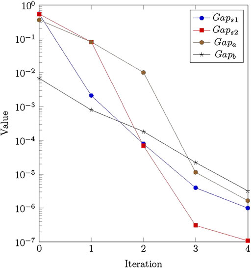
FIGURE 5. Relaxation gap’s change during iterations.

In summary, the proposed method is tested on a real offshore wind system. Both the power loss of the transmission lines and the relaxation gap are reduced by iterations of the convex–concave procedure.

5 Conclusion

In this article, a convex–concave procedure-based method for the optimal power flow of offshore wind farms is proposed.

1) It is established with the relaxation variables.

2) Two sets of the inequality constraints are implemented to replace the nonlinear and non-convex equality constraints.

3) To drive the gap of the second-order cone relaxations to be zero, the first-order Taylor expansion-based iteration is imposed.

From the test results of the real wind farm, the superiority of the proposed method is verified. It can be found that the proposed method can optimize the power loss of the transmission lines and improve the power transmitted to the power grid. Moreover, the relaxation gap is tested to be around zero with the proposed iterations.

In the future work, this method will be improved with high solving efficiency.

Data Availability Statement

The original contributions presented in the study are included in the article/Supplementary Material; further inquiries can be directed to the corresponding author.

Author Contributions

YC: methodology, software, visualization, writing—original draft preparation, and writing—reviewing and editing. HL: supervision and writing—reviewing and editing. QC: methodology and software. RX: methodology and reviewing. XW: visualization and reviewing.

Funding

This project was supported by the National Key R&D Program of China (2021YFB2400600).

Conflict of Interest

YC, HL, QC, RX, and XW were employed by the company PowerChina Huadong Engineering Corporation Limited.

Publisher’s Note

All claims expressed in this article are solely those of the authors and do not necessarily represent those of their affiliated organizations, or those of the publisher, the editors, and the reviewers. Any product that may be evaluated in this article, or claim that may be made by its manufacturer, is not guaranteed or endorsed by the publisher.

References

Abdelouadoud, S. Y., Girard, R., Neirac, F. P., and Guiot, T. (2015). Optimal Power Flow of a Distribution System Based on Increasingly Tight Cutting Planes Added to a Second Order Cone Relaxation. Int. J. Electr. Power and Energy Syst. 69, 9–17. doi:10.1016/j.ijepes.2014.12.084

CrossRef Full Text | Google Scholar

Apostolaki-Iosifidou, E., Mccormack, R., Kempton, W., Mccoy, P., and Ozkan, D. (2019). Transmission Design and Analysis for Large-Scale Offshore Wind Energy Development. IEEE Power Energy Technol. Syst. J. 6, 22–31. doi:10.1109/jpets.2019.2898688

CrossRef Full Text | Google Scholar

Bourguignon, S., Ninin, J., Carfantan, H., and Mongeau, M. (2015). Exact Sparse Approximation Problems via Mixed-Integer Programming: Formulations and Computational Performance. IEEE Trans. Signal Process. 64, 1405–1419. doi:10.1109/TSP.2015.2496367

CrossRef Full Text | Google Scholar

Boyd, S., Boyd, S. P., and Vandenberghe, L. (2004). Convex Optimization. Los Angeles: Cambridge University Press.

Google Scholar

Chen, Y., Xiang, J., and Li, Y. (2021). A Quadratic Voltage Model for Optimal Power Flow of a Class of Meshed Networks. Int. J. Electr. Power and Energy Syst. 131, 107047. doi:10.1016/j.ijepes.2021.107047

CrossRef Full Text | Google Scholar

Cremers, D., and Kolev, K. (2010). Multiview Stereo and Silhouette Consistency via Convex Functionals over Convex Domains. IEEE Trans. Pattern Anal. Mach. Intell. 33, 1161–1174. doi:10.1109/TPAMI.2010.174

PubMed Abstract | CrossRef Full Text | Google Scholar

Fazlyab, M., Paternain, S., Preciado, V. M., and Ribeiro, A. (2017). Prediction-Correction Interior-point Method for Time-Varying Convex Optimization. IEEE Trans. Automatic Control 63, 1973–1986.

Google Scholar

Goli, A., Khademi-Zare, H., Tavakkoli-Moghaddam, R., Sadeghieh, A., Sasanian, M., and Malekalipour Kordestanizadeh, R. (2021). An Integrated Approach Based on Artificial Intelligence and Novel Meta-Heuristic Algorithms to Predict Demand for Dairy Products: a Case Study. Netw. Comput. Neural Syst. 32, 1–35. doi:10.1080/0954898x.2020.1849841

CrossRef Full Text | Google Scholar

Guirguis, D., Romero, D. A., and Amon, C. H. (2016). Toward Efficient Optimization of Wind Farm Layouts: Utilizing Exact Gradient Information. Appl. Energy 179, 110–123. doi:10.1016/j.apenergy.2016.06.101

CrossRef Full Text | Google Scholar

Hijazi, H., Coffrin, C., and Hentenryck, P. V. (2017). Convex Quadratic Relaxations for Mixed-Integer Nonlinear Programs in Power Systems. Math. Prog. Comp. 9, 321–367. doi:10.1007/s12532-016-0112-z

CrossRef Full Text | Google Scholar

Jubril, A. M., Olaniyan, O. A., Komolafe, O. A., and Ogunbona, P. O. (2014). Economic-emission Dispatch Problem: A Semi-definite Programming Approach. Appl. Energy 134, 446–455. doi:10.1016/j.apenergy.2014.08.024

CrossRef Full Text | Google Scholar

Khan, A., Naeem, M., Iqbal, M., Qaisar, S., and Anpalagan, A. (2016). A Compendium of Optimization Objectives, Constraints, Tools and Algorithms for Energy Management in Microgrids. Renew. Sustain. Energy Rev. 58, 1664–1683. doi:10.1016/j.rser.2015.12.259

CrossRef Full Text | Google Scholar

Konar, A., and Sidiropoulos, N. D. (2017). First-order Methods for Fast Feasibility Pursuit of Non-Convex Qcqps. IEEE Trans. Signal Process. 65, 5927–5941. doi:10.1109/tsp.2017.2736516

CrossRef Full Text | Google Scholar

Li, Q., Yu, S., Al-Sumaiti, A. S., and Turitsyn, K. (2018). Micro Water–Energy Nexus: Optimal Demand-Side Management and Quasi-Convex Hull Relaxation. IEEE Trans. Control Netw. Syst. 6, 1313–1322.

Google Scholar

Li, Y., Xiao, J., Chen, C., Tan, Y., and Cao, Y. (2018). Service Restoration Model with Mixed-Integer Second-Order Cone Programming for Distribution Network with Distributed Generations. IEEE Trans. Smart Grid 10, 4138–4150.

Google Scholar

Li, Y., Zhang, H., Huang, B., and Han, J. (2020). A Distributed Newton-Raphson-based Coordination Algorithm for Multi-Agent Optimization with Discrete-Time Communication. Neural Comput. Applic 32, 4649–4663. doi:10.1007/s00521-018-3798-1

CrossRef Full Text | Google Scholar

Li, Z., Xu, Y., Fang, S., Zheng, X., and Feng, X. (2020). Robust Coordination of a Hybrid Ac/dc Multi-Energy Ship Microgrid with Flexible Voyage and Thermal Loads. IEEE Trans. Smart Grid 11, 2782–2793. doi:10.1109/tsg.2020.2964831

CrossRef Full Text | Google Scholar

Li, Z., Wu, L., Xu, Y., Moazeni, S., and Tang, Z. (2022). Multi-stage Real-Time Operation of a Multi-Energy Microgrid with Electrical and Thermal Energy Storage Assets: A Data-Driven Mpc-Adp Approach. IEEE Trans. Smart Grid 13, 213–226. doi:10.1109/TSG.2021.3119972

CrossRef Full Text | Google Scholar

Lofberg, J. (2004). “YALMIP : A Toolbox for Modeling and Optimization in MATLAB,” 2004 IEEE International Conference on Robotics and Automation (IEEE Cat. No.04CH37508) 41, 284–289. doi:10.1109/CACSD.2004.1393890

CrossRef Full Text | Google Scholar

Ma, M., Fan, L., Miao, Z., Zeng, B., and Ghassempour, H. (2020). A Sparse Convex Ac Opf Solver and Convex Iteration Implementation Based on 3-node Cycles. Electr. Power Syst. Res. 180, 106169. doi:10.1016/j.epsr.2019.106169

CrossRef Full Text | Google Scholar

Neftci, E. O., Mostafa, H., and Zenke, F. (2019). Surrogate Gradient Learning in Spiking Neural Networks: Bringing the Power of Gradient-Based Optimization to Spiking Neural Networks. IEEE Signal Process. Mag. 36, 51–63. doi:10.1109/msp.2019.2931595

CrossRef Full Text | Google Scholar

Rokbani, N., Kumar, R., Abraham, A., Alimi, A. M., Long, H. V., Priyadarshini, I., et al. (2021). Bi-heuristic Ant Colony Optimization-Based Approaches for Traveling Salesman Problem. Soft Comput. 25, 3775–3794. doi:10.1007/s00500-020-05406-5

CrossRef Full Text | Google Scholar

Ruan, G., Zhong, H., Wang, J., Xia, Q., and Kang, C. (2020). Neural-network-based Lagrange Multiplier Selection for Distributed Demand Response in Smart Grid. Appl. Energy 264, 114636. doi:10.1016/j.apenergy.2020.114636

CrossRef Full Text | Google Scholar

Shafiee, M. (2015). Maintenance Logistics Organization for Offshore Wind Energy: Current Progress and Future Perspectives. Renew. energy 77, 182–193. doi:10.1016/j.renene.2014.11.045

CrossRef Full Text | Google Scholar

Shinano, Y., and Fujie, T. (2007). Paralex:a Parallel Extension for the Cplex Mixed Integer Optimizer. Recent Adv. Parallel Virtual Mach. Message Passing Interface 4757, 97–106. doi:10.1007/978-3-540-75416-9_19

CrossRef Full Text | Google Scholar

Xie, S., Xu, Y., and Zheng, X. (2022). On Dynamic Network Equilibrium of a Coupled Power and Transportation Network. IEEE Trans. Smart Grid 13, 1398–1411. doi:10.1109/tsg.2021.3130384

CrossRef Full Text | Google Scholar

Zhang, D., Wang, J., Lin, Y., Si, Y., Huang, C., Yang, J., et al. (2017). Present Situation and Future Prospect of Renewable Energy in china. Renew. Sustain. Energy Rev. 76, 865–871. doi:10.1016/j.rser.2017.03.023

CrossRef Full Text | Google Scholar