Collaborative optimization of train timetable and speed trajectory considering stochastic photovoltaic power: A two-step approach

Faced with the integrated system composed of the train power system, the photovoltaic (PV) power system, and the energy storage system (ESS), this research studies the energy-efficient operation and energy management strategy from the perspective of both train optimal control and timetable optimization, aiming at achieving a long-term energy consumption reduction. A two-step approach for collaboratively optimizing the train timetable, speed trajectory, and energy management strategy considering the stochastic characteristics of PV power generation is proposed to solve this large-scale complex problem. Before the two-step approach, a mixed-integer linear programming (MILP) model is established to optimize the energy consumption of the inter-station operation. On this basis, explicit energy consumption expressions for all inter-stations of the entire line are obtained by the proposed data fitting method. The historical PV power data is clustered to generate scenarios with different probabilities to characterize the stochastic PV power. The first step of this two-step approach is to minimize the total energy consumption expectations of all inter-stations determined by the obtained explicit energy consumption expressions to optimize the timetable while ensuring the total time and time window constraints are met. The second step is to minimize the weighted sum of energy consumption under all possible scenarios to obtain the optimal speed trajectory and energy management strategy based on the optimized timetable obtained in the first step. The validity of the model is verified by case studies using the real data of Qingdao Metro Line 11 under both scenarios with and without PV power. This study provides a novel method for energy-efficient operation and energy management of the integrated system and demonstrates the prospect of the proposed two-step stochastic optimization in reducing the net grid-supplied energy for the long-term operation of urban rail transportation systems.

1 Introduction

Renewable energy is considered as a clean and safe alternative to fossil fuels to alleviate the energy crisis and reduce carbon emissions. System integration with the renewable energy system is an effective solution to the sustainable development of energy systems (Ehteshami et al., 2022). Photovoltaic (PV) power due to its outstanding economic and environmental benefits, is considered to have great potential in the field of system integration with the energy storage system (ESS) and train traction system (Shen et al., 2020). However, the integration of renewable energy systems and the ESS demands intimate coupling between different systems, which brings new challenges to energy-efficient train control (EETC) and energy management. For example, the PV power generation and the energy consumption demand of the train traction system are intermittent. The increase in the permeability of renewable energy in the system structure may cause it difficult for the system operations to match the power supply and demand (Kanchev et al., 2014). Improving the efficiency of the integrated system has become more and more important in its sustainable development and is expected to attract much more attention in the near future.

Timetable optimization and train speed trajectory optimization are two main branches of existing research on EETC (Scheepmaker et al., 2017).

For timetable optimization, the mixed-integer nonlinear programming model was used to optimize the timetable, and an efficient hybrid optimization algorithm based on particle swarm optimization and simulated annealing was designed to obtain the approximate optimal solution effectively (Guo et al., 2017). Montrone et al. (2018) proposed a model to realize real-time timetable optimization. The model searches the combination of the train regimes to dynamically adjust the timetable to minimize energy consumption. Liu et al. (2018) studied the train schedule problem of the integration of the subway system and the ESS, aiming to maximize the use of regenerative braking energy. The nonlinear integer programming model was adopted, and the tabu search algorithm and the hybrid simulation algorithm were designed to solve the problem.

For speed trajectory optimization, in (Lu et al., 2013), a speed trajectory search space modeling process was proposed. Ant colony algorithm, genetic algorithm, and dynamic programming algorithm were used to solve the problem. The results of various models were analyzed and compared. Huang et al. (2018) and Wu et al. (2019) studied the speed trajectory optimization model considering the ESS using dynamic programming and mixed-integer linear programming, respectively. It was considered that the regenerative energy generated by the braking train could be stored in the ESS and provided for the subsequent traction operation.

Although the speed trajectory and timetable optimization have been extensively studied, they interact with each other and the optimization of them separately cannot achieve the best energy-saving effect. Therefore, some studies were devoted to collaborative optimization of train speed trajectory and timetable. Su et al. (2013) proposed a bi-level programming model, and an iterative method was used to optimize the time and train speed profile of the two to save the energy consumption of the whole line. Wang et al. (2021) transformed collaborative optimization into a discrete decision problem based on the space-time-speed network method. The global optimal solution was obtained by the dynamic programming algorithm, and the approximate optimal solution was quickly obtained by the discrete difference dynamic programming algorithm. Wu et al. (2021) proposed a two-step optimization method that considered collaborative optimization of speed trajectory and timetable with the integration of the ESS, which could not only obtain the optimal timetable and speed trajectory but also obtain the charging and discharging strategy of the ESS.

Based on the above studies, it can be seen that the optimization of speed trajectory and the optimal allocation of the timetable have been extensively studied. The collaborative optimization of the two can achieve better results, which is considered to be an interesting research direction. However, most of the above studies on EETC are limited to the traction system. We have seen that there have been studies on EETC combined with the ESS, but there are much fewer studies on the impact of renewable energy system integration. However, the system’s net energy consumption is determined by a series of interdependent factors. Consequently, the optimization of integrated systems should be paid more attention to, not limited to the energy-saving of subsystems (González-Gil et al., 2014).

Kaffash et al. (2021) proposed a data-driven method to obtain the distribution of random PV power and generate the uncertainty scenario set of PV power generation. This method was based only on historical PV power data. The generated scenario sets were used as input, and two-step stochastic optimization was used to study the PV cell system management problem. And it was tested in the PV cell system scheduling of commercial buildings. Park and Salkuti (2019) proposed an energy management system to manage energy flow by coordinating the train operation, renewable energy system, the ESS, and the grid. Using mixed integer linear stochastic programming, a model of railway station energy management system considering the ESS, regenerative braking energy, PV power generation, and the power grid was established in (Şengör et al., 2017). Similarly, Aguado et al. (2018) considered the stochastic characteristics of renewable energy through the scenario tree method and studied the optimization operation of the integrated railway system. A large-scale nonlinear optimization model was established to study the efficient operation of the railway and the ESS.

Based on the above literature review, the collaborative optimization of the speed trajectory and the timetable are not studied thoroughly in the context of integrated system planning. The coupling of renewable energy systems is rarely considered in the study of EETC. Therefore, it is an interesting problem to optimize the train operation from both speed trajectory and timetable perspectives for the entire railway line considering the integration of PV, the ESS, and the train traction system in order to further improve the energy-saving performance of the system.

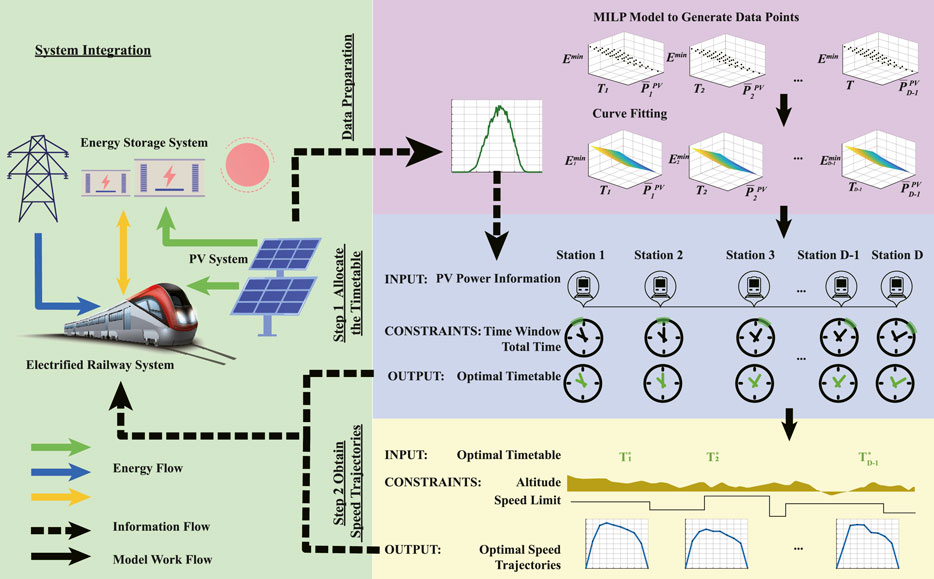
This paper proposes a two-step approach to solve the large-scale nonlinear stochastic problem with high computational complexity. To indicate the scope and framework of this research more clearly, the system integration scheme and the two-step approach framework are demonstrated in Figure 1. The green block shows the energy flow pattern of the integrated system, where the solid and colored arrows represent the direction of the energy flow. The power of train traction is provided by the power grid, the ESS, and the PV system. The ESS can recover the regenerative braking energy when the train is braking and absorb the surplus PV power. The three blocks on the right show the workflow of the model. The pink block demonstrates the data preparation process. The minimum energy consumption model for the inter-station operation based on MILP is proposed. Then, a series of data points are generated by solving the MILP model under different input combinations of operation time and PV power. The energy consumption for each combination corresponds to a data point. Subsequently, an explicit relationship among the energy consumption, time, and PV power is obtained by data fitting. The stochastic PV power is characterized by different scenarios generated by historical PV power data clustering, which is used as the model input. The blue block shows Step 1, where the energy consumption expectation of the whole line is minimized under the constraints of the time window and total time to obtain the optimal timetable. The yellow block presents Step 2, where the optimal train operation and energy management strategy for the entire railway line are acquired through MILP models for all inter-station operations.

FIGURE 1

FIGURE 1. Schematic of the system energy flow and model framework.

The study proposed in this paper mainly contributes to the field in the following two aspects:

1 With a consideration on integrated PV power generation into the urban rail transportation, the EETC and energy management of the integrated system composing of the train traction system and ESS are studied. The train speed trajectory, timetable, and energy management strategy are collaboratively optimized to realize the long-term energy-saving effect of the integrated system.

2 A two-step approach is proposed to solve the large-scale stochastic optimization problem, which improves the computational efficiency. The historical data clustering is used to generate scenarios to characterize the stochastic PV power, which tackles the intermittency of the PV power generation. The proposed two-step approach has a low requirement for PV power prediction with strong applicability and practicability.

The rest of the paper is organized as follows: In Section 2, the establishment of the MILP model is introduced. Section 3 demonstrates the algorithm of the two-step approach. In Section 4, the real data is used to do case analysis. Monte Carlo long-term operation simulation is carried out to verify the model’s effectiveness and robustness and analyze the energy-saving effect. Conclusions are drawn in Section 5.

2 Mixed-integer linear programming model for operation between two stations

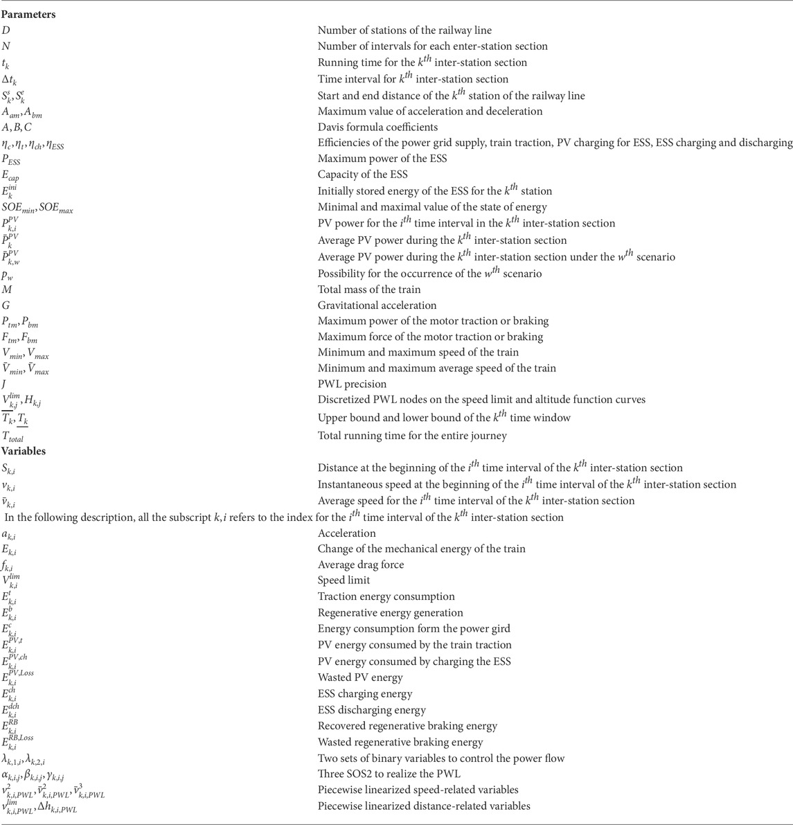
This section proposes an optimization method of the speed trajectory, timetable, and energy management between two stations considering PV power generation and energy storage system (ESS) based on MILP. The nomenclature of parameters and variables are listed in Table 1.

TABLE 1

TABLE 1. Nomenclature.

2.1 Kinematics modeling of the train

Suppose there are D stations in the entire railway line and D − 1 inter-station sections. Every inter-station section is time-equally divided into N intervals, where N determines the model precision. The train is assumed to be uniformly accelerated in these intervals. A balance between model accuracy and complexity can be achieved by choosing an appropriate value of N. For the sake of clarity, subscript k, i denotes the i^th interval of the k^th inter-station section. Punctuality of the train for each inter-station is ensured by Eqs. 1, 2.

$S_{k,1}=S_k^s(1)$

$S_{k,N+1}=S_k^e(2)$

$S_k^s$ and $S_k^e$ are the starting and ending position of the k^th section of the journey, k = 1, 2, … , D − 1. The position, average speed, and acceleration are calculated as Eqs. 3–5, where ${\bar{v}}_{k,j}$ is the average speed of the i^th period of the k^th section, v_k,i is the speed at the beginning of the i^th period of the k^th section.

$S_{k,i+1}=S_{k,1}+\sum _{j=1}^i{\bar{v}}_{k,j}\mathrm{\Delta }{t}_k,i=\mathrm{1,2,3},\dots ,N(3)$

${\bar{v}}_{k,i}=\frac{v_{k,i}+v_{k,i+1}}{2}(4)$

$a_{k,i}=\frac{v_{k,i+1}-v_{k,i}}{\mathrm{\Delta }{t}_k}(5)$

The operation time is t_k for the k^th inter-station operation. For every interval, the period of time is Δt_k = t_k/N. The magnitude of the acceleration is limited as Eq. 6, 7 to ensure passenger comfort.

$a_{k,i}\le A_{am}(6)$

$-a_{k,i}\le A_{bm}(7)$

A_am and A_bm are the maximum values of acceleration and deceleration. The drag force during train travels is expressed by Davis formula (Scheepmaker et al., 2017) shown in Eq. 8. The value of coefficients A, B and C are referred from Wu et al. (2019).

$f_{k,i}=A+B{\bar{v}}_{k,i}+C{\bar{v}}_{k,i}^2(8)$

The train is required to operate at the speed under the limit, as Eq. 9 shows.

$v_{k,i}\le V_{k,i}^{\lim }(9)$

$V_{k,i}^{\lim }$ is the speed limit, which is regarded as a function related to distance.

2.2 Energy flow management modeling

For the convenience of description, the energy consumption of the train power system is divided into two parts, namely the consumption during traction $E_{k,i}^t,E_{k,i}^t>0$ and the consumption during braking $E_{k,i}^b,E_{k,i}^b\le 0$. The coasting regime is also be included in $E_{k,i}^b$, when $E_{k,i}^b=0$, which means that the train traction system does not consume or generate energy.

During the traction phase, according to the energy flow mode shown in Figure 1, the energy consumption can be expressed as Eq. 10.

$E_{k,i}^t=E_{k,i}^c{\eta }_c+E_{k,i}^{PV,t}{\eta }_t+E_{k,i}^{\mathit{dch}}{\eta }_{\mathit{ESS}}(10)$

$E_{k,i}^c,E_{k,i}^{PV,t},E_{k,i}^{\mathit{dch}}$ are energy consumed from the power grid, PV power system, and the ESS, respectively. η_c, η_t, η_ESS are the according efficiencies. During the braking phase, the train traction system is regarded as the energy source due to the regenerative braking, as shown in Eq. 11. Regenerative braking energy may be inadequately recovered.

$-E_{k,i}^b=E_{k,i}^{RB}+E_{k,i}^{RB,Loss}(11)$

$E_{k,i}^{RB}$ is the energy that can be recovered. $E_{k,i}^{RB,Loss}$ is the energy that cannot be recovered constrained by the ESS power and capacity, which is consumed as heat. The energy recovered by the ESS comes from the regenerative braking energy $E_{k,i}^{RB}$ and PV power energy to charge the system $E_{k,i}^{PV,ch}$, as shown in Eq. 12.

$E_{k,i}^{ch}\le E_{k,i}^{RB}{\eta }_{\mathit{ESS}}+E_{k,i}^{PV,ch}{\eta }_{ch}(12)$

Due to the constraints of ESS power, the charging and discharging energy are constrained to Eq. 13, 14.

$E_{k,i}^{\mathit{dch}}\le P_{\mathit{ESS}}\mathrm{\Delta }{t}_k(13)$

$E_{k,i}^{ch}\le P_{\mathit{ESS}}\mathrm{\Delta }{t}_k(14)$

P_ESS is the maximum power of ESS charging or discharging. The state of energy of the ESS is shown in Eq. 15, it has the range as Eq. 16 shows.

$SO{E}_{k,i}=\left\{\begin{array}{c}\hfill \frac{E_k^{\mathit{ini}}}{E_{\mathit{cap}}},i=0\hfill \\ \hfill \frac{E_k^{\mathit{ini}}+{\sum }_{\mathit{j}=1}^i{E}_{k,j}^{ch}-{\sum }_{\mathit{j}=1}^i{E}_{k,j}^{\mathit{dch}}}{E_{\mathit{cap}}}i=\mathrm{1,2},\dots ,N\hfill \end{array}\right.(15)$

$SO{E}_{\min }\le SO{E}_{k,i}\le SO{E}_{\max }(16)$

$E_k^{\mathit{ini}}$ is the initial energy stored in the ESS, E_cap is the ESS capacity. SOE_min and SOE_max are the minimum and maximum state of energy of the ESS. For the PV power system, the energy conservation is determined by Eq. 17.

$E_{k,i}^{PV,t}+E_{k,i}^{PV,ch}+E_{k,i}^{PV,Loss}=P_{k,i}^{PV}\mathrm{\Delta }{t}_k(17)$

$P_{k,i}^{PV}$ is the PV output power, it is consumed by train traction or ESS charging, which is $E_{k,i}^{PV,t}$ and $E_{k,i}^{PV,ch}$, respectively. $E_{k,i}^{PV,Loss}$ is the PV energy that cannot be fully utilized. For the train power system, the energy conservation is shown in Eq. 18, where E_k,i is $E_{k,i}^t$ during traction and $E_{k,i}^b$ during braking.

$E_{k,i}-\frac{1}{2}M\left(v_{k,i+1}^2-v_{k,i}^2\right)-f_{k,i}{\bar{v}}_{k,i}\mathrm{\Delta }{t}_k-Mg\mathrm{\Delta }{h}_{k,i}\ge 0(18)$

M is the total mass of the train, g is the gravitational acceleration. Δh_k,i is the altitude change of the railway line. Eqs. 19–22 are the constraints of motor for traction system from both force and power perspectives.

$E_{k,i}^t\le P_{tm}\mathrm{\Delta }{t}_k(19)$

$-E_{k,i}^b\le P_{bm}\mathrm{\Delta }{t}_k(20)$

$E_{k,i}^t\le F_{tm}{\bar{v}}_{k,j}\mathrm{\Delta }{t}_k(21)$

$-E_{k,i}^b\le F_{bm}{\bar{v}}_{k,j}\mathrm{\Delta }{t}_k(22)$

P_tm and P_bm are the maximum power for traction and breaking. F_tm and F_bm are the maximum traction and braking force. Eqs. 23, 24 are used to control the energy flow of the train traction power system and the ESS.

$E_{k,i}={\lambda }_{k,1,i}{E}_{k,i}^t+\left(1-{\lambda }_{k,1,i}\right)E_{k,i}^b(23)$

λ_k,1,i, λ_k,2,i are two independent binary variables. Eq. 23 ensures that E_k,i can only be either $E_{k,i}^t$ (when λ_k,1,i = 1) or $E_{k,i}^b$ (when λ_k,1,i = 0), which means that the train can only be in either traction phase or braking phase. Eq. 24 are to ensure that the power grid, PV power system, and ESS do not provide energy for train traction under coasting or braking phase.

$\left\{\begin{array}{c}{E}_{k,i}^c=0\hfill \\ E_{k,i}^{\mathit{dch}}=0{\lambda }_{k,1,i}=0\hfill \\ E_{k,i}^{PV,t}=0\hfill \end{array}\right.(24)$

Eqs 25, 26 prevent simultaneous charging and discharging of ESS.

$\begin{array}{cc}\hfill E_{k,i}^{\mathit{dch}}=0\hfill & \hfill {\lambda }_{k,2,i}=0\hfill \end{array}(25)$

$\begin{array}{cc}\hfill E_{k,i}^{ch}=0\hfill & \hfill {\lambda }_{k,2,i}=1\hfill \end{array}(26)$

So far, the model has been constructed. However, there are nonlinear terms in the constraints, which need to be linearized in the following section by the piecewise linearization (PWL) technique.

2.3 Piecewise linearization approach

The piecewise linear (PWL) method is used to linearize the nonlinear constraints in the above-mentioned model, so as to reduce the complexity and improve the computational efficiency. The special ordered set of type 2 (SOS2) is used to realize the linearization. Suppose there are three groups of SOS2 α_k,i, β_k,i, γ_k,i corresponding to the variables which need to be linearized at i^th interval in the k^th section. The subscript j denotes the j^th elements in that SOS2. j ranges from 1 to J where J is the piecewise precision. k ranges from 1 to D − 1. The range of i is consistent with the linearized variable. If no range is specified, all the following subscripts indicate that the formula is applicable to any subscript in its range. In SOS2, there are at most two elements that are non-zero. If there are two, they must be adjacent. Others are all zero. Eqs. 27, 28 are constraints added to realize the PWL process. The same with β_k,i,j as shown in Eqs. 29, 30 and γ_k,i,j as shown in Eqs. 31, 32.

$\sum _{j=0}^J{\alpha }_{k,i,j}=1(27)$

$0\le {\alpha }_{k,i,j}\le 1,j=\mathrm{0,1,2},\dots ,J(28)$

$\sum _{j=0}^J{\beta }_{k,i,j}=1(29)$

$0\le {\beta }_{k,i,j}\le 1,j=\mathrm{0,1,2},\dots ,J(30)$

$\sum _{j=0}^J{\gamma }_{k,i,j}=1(31)$

$0\le {\gamma }_{k,i,j}\le 1,j=\mathrm{0,1,2},\dots ,J(32)$

Eq. 33 shows the process of linearizing the instantaneous speed square.

$v_{k,i,PWL}^2=\sum _{j=0}^J{\left[V_{\min }+j\left(\frac{V_{\max }-V_{\min }}{J}\right)\right]}^2{\alpha }_{k,i,j}(33)$

V_min, V_max are the minimum and maximum value are the lower and upper limits of the PWL range, which are constant. Similarly, Eqs. 34, 35 shows the linearization for average speed square and cube.

${\bar{v}}_{k,i,PWL}^2=\sum _{j=0}^J{\left[{\bar{V}}_{\min }+j\left(\frac{{\bar{V}}_{\max }-{\bar{V}}_{\min }}{J}\right)\right]}^2{\beta }_{k,i,j}(34)$

${\bar{v}}_{k,i,PWL}^3=\sum _{j=0}^J{\left[{\bar{V}}_{\min }+j\left(\frac{{\bar{V}}_{\max }-{\bar{V}}_{\min }}{J}\right)\right]}^3{\beta }_{k,i,j}(35)$

Replace $v_{k,i}^2,{\bar{v}}_{k,i}^2,{\bar{v}}_{k,i}^3$ with $v_{k,i,PWL}^2,{\bar{v}}_{k,i,PWL}^2,{\bar{v}}_{k,i,PWL}^3$, respectively, all nonlinear terms related to speed and average speed in Eqs. 8–18 are linearized.

In addition, the altitude and speed limit are nonlinear functions related to distance and the corresponding relationship between distance and time needs to be established in our time-based model. Eq. 36 combined with Eq. 3 builds a relationship between time and distance by SOS2 variables γ_k,i.

$S_{k,i}=\sum _{j=0}^{J}j\left(\frac{S_k^e-S_k^s}{J}\right){\gamma }_{k,i,j}(36)$

$v_{k,i,PWL}^{\lim }=f\left(S_{k,i}\right)=\sum _{j=0}^J{V}_{k,j}^{\lim }{\gamma }_{k,i,j}(37)$

$\begin{array}{ll}\hfill \mathrm{\Delta }{h}_{k,i,PWL}=g\left(S_{k,i+1}\right)-g\left(S_{k,i}\right)& =\sum _{j=0}^J{H}_{k,j}{\gamma }_{k,i+1}^j\hfill \\ \hfill & -\sum _{j=0}^J{H}_{k,j}{\gamma }_{k,i,j}\hfill \end{array}(38)$

f(S), g(S) are the piecewise functions representing the speed limit and altitude, and $V_{k,j}^{\lim },H_{k,j}$ are discretized points on f(S), g(S), respectively. Eqs. 37, 38 realize the linearization for the altitude and speed limit by replacing $v_{k,i}^{\lim },\mathrm{\Delta }{h}_{k,i}$ in Eqs. 9–18 with $V_{k,i,PWL}^{\lim },\mathrm{\Delta }{h}_{k,i,PWL}$. So far, all nonlinear constraints have been linearized.

2.4 Stochastic optimization considering intermittent PV power

$P_{k,i}^{PV}$ is uncertain in Eq. 17. To consider the stochastic behavior of the PV power, historical PV power generation data are used for clustering to generate different scenarios. Each scenario represents a specific type of generated weather. Suppose there are W scenarios generated by the historical data, for each scenario, the net energy consumption can be written as Eq. 39, where ${\bar{P}}_k^{PV}=\sum _{i=1}^N{P}_{k,i}^{PV}/N$. As a renewable energy, PV power is free and thus not involved in the net energy consumption. The difference between the total charge and discharge energy $\sum _{i=1}^N{E}_{k,i}^{ch}-\sum _{i=1}^N{E}_{k,i}^{\mathit{dch}}$ is the energy stored in the ESS, which can be consumed in the subsequent operation. For that reason, it is subtracted from the energy provided by the grid. As a result, the net energy consumption shown in Eq. 39 is equivalent to the net energy supplied by the grid. In this paper, net energy consumption and net grid-supplied energy are interchangeable.

$\begin{array}{ll}\hfill e_k\left({\bar{P}}_k^{PV}\right)& =\sum _{i=1}^N{E}_{k,i}^c-\left(\sum _{i=1}^N{E}_{k,i}^{ch}-\sum _{i=1}^N{E}_{k,i}^{\mathit{dch}}\right)\hfill \\ \hfill & =\sum _{i=1}^N{E}_{k,i}^c-\sum _{i=1}^N{E}_{k,i}^{ch}+\sum _{i=1}^N{E}_{k,i}^{\mathit{dch}}\hfill \end{array}(39)$

For each scenario, there is one corresponding net energy consumption expression with the form of Eq. 39. The objective of stochastic optimization is to minimize the expected net energy consumption in all scenarios. In that case, the optimal solution obtained by the stochastic optimization is expected to perform well no matter how the future PV power changes. The stochastic optimization objective function is the expectation of Eq. 39, namely Eq. 40.

$obj=E\left(e_k\left({\bar{P}}_k^{PV}\right)\right)=\sum _{w=1}^{w=W}{p}_w{e}_k\left({\bar{P}}_{k,w}^{PV}\right)(40)$

W is the number of scenarios. p_w and $e_k({\bar{P}}_{k,w}^{PV})$ are the probability of the occurrence of the w^th scenario and the corresponding net energy consumption, respectively.

3 A two-step optimization approach for the entire railway line

3.1 Data points generation and surface Fitting

Firstly, we assume that the influences of scheduled time and PV power on the net energy consumption are mutually independent and the superposition of the two determines the minimum net energy consumption. Secondly, the objective of this study is to give the long-term optimal control strategy of the integrated system by stochastic optimization. From this viewpoint, the consideration of real-time PV power is not necessary. Moreover, the ESS can compensate for the uncertainty caused by stochastic optimization. So, the average power of PV during the scheduled time is the independent variable. Therefore, we assume that the general relationship between the minimum energy consumption concerning the scheduled time and PV power has the form of Eq. 41.

$E_k^{\min }=f_k\left(T\right)+g_k\left({\bar{P}}^{PV}\right)(41)$

Another obvious advantage of using the average PV power is avoiding repeated fittings when the PV power condition changes. It is only needed to calculate the average PV power according to the scheduled time as input before the fitting process. When we perform optimization for a specified railway line, the fitting parameters only depend on the system itself and are independent of the input PV power time-series data. Therefore, we only need to fit once to obtain the characteristics of the train operation energy consumption. This avoids the trouble of repeated fitting since a large number of data points are generated through the MILP model before each fitting process, which is time-consuming.

In addition, it is notable that although we calculate the average PV power according to the time before the timetable optimization, this has little effect on the model accuracy. The reason is that the time window is relatively short on a scale of seconds, during which the PV power will not change dramatically, compared with the PV prediction time scale in minutes or hours.

Wu et al. (2021) studied the relationship between the minimum net energy consumption and the inter-station operation time and suggested using the modified inverse function for fitting, namely f_k(T) = A_k + B_k/(C_k + T). We use a specific case with a journey of 1.8 km and a scheduled time of 112 s to verify this result. The corresponding minimum net energy consumption is obtained and fitted according to the formula f_k(T) = A_k + B_k/(C_k + T) by changing the operation time. The results are shown in Figure 2A. The parameters are A_k = 18.89, B_k = 590.4, C_k = −79.4 and the performance is R² = 0.9994. The results show that it is feasible to approximate the relationship between E^min and T with the modified inverse function. Without loss of generality, the increase in PV power is assumed to reduce the net energy consumption linearly. This assumption is based on the reality that PV power is not too sufficient to lead to great energy waste. Therefore, the overall utilization rate of PV power will not decrease significantly due to the increase of the PV power within the scope of our research interest. This suggests that $g_k({\bar{P}}^{PV})=D_k+E_k{\bar{P}}^{PV}$. The same special case is used for verification. The results are shown in Figure 2B The parameters are D_k = 45.7, E_k = −0.1013. The performance is R² = 0.9997. These results imply that the modified inverse and linear function can separately estimate the energy consumption versus time and PV power. Therefore, $E_k^{\min }(T,{\bar{P}}^{PV})$ can be expressed as Eq. 42 after parameters combination.

$E_k^{\min }=A_k+\frac{B_k}{C_k+T}+D_k{\bar{P}}^{PV}(42)$

FIGURE 2

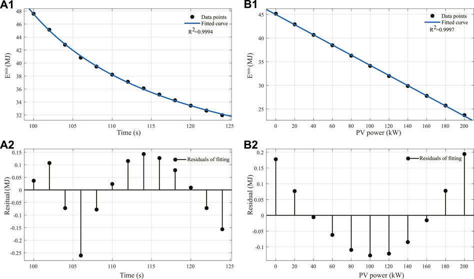
FIGURE 2. Fit performance of E^min versus time and PV power. (A1) Fit result of E^min versus time. (A2) Corresponding residual. (B1) Fit result of E^min versus PV power. (B2) Corresponding residual.

The stochastic PV power can be characterized by different scenarios and their probabilities. Note that Eq. 42 is explicit and the term ${\bar{P}}^{PV}$ is linear. Therefore, we can directly write the expectation of the objective function for the stochastic optimization model considering multiple scenarios as Eq. 43 shows.

$\begin{array}{ll}\hfill E\left(E_k^{\min }\right)=A_k+\frac{B_k}{C_k+T}+D_{k}E\left({\bar{P}}^{PV}\right)& =A_k+\frac{B_k}{C_k+T}\hfill \\ \hfill & +D_k\sum _{w=1}^W{p}_w{\bar{P}}_w^{PV}\hfill \end{array}(43)$

An example for generating data points and fitting the surface is shown in Figure 3, which is the result for the inter-station operation from Station HZZX to Station QDEZ. We select the real line data of Qingdao Metro Line 11 (22 stations) and apply the MILP model mentioned above with various combinations of the time and PV power to obtain a matrix of 3D spatial data points $E^{\min }(T,{\bar{P}}^{PV})$, as shown in the black points in Figure 3A. Then fit the surface according to Eq. 42 using the least square method to obtain the fitted curve as shown in the surface in Figure 3A. Figure 3B shows the corresponding residuals. The fitting parameters and performances for the entire railway line are shown in Table 2. The abbreviations are the station names, such as MLL, HZZX, etc. It is observed that all the R² values are larger than 0.95, indicating a good fitting performance.

FIGURE 3

FIGURE 3. Data fitting results for the inter-station operation from Station HZZX to Station QDEZ. (A) Generated data points and fitted surface. (B) Residual plot.

TABLE 2

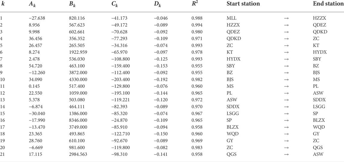
TABLE 2. Fitting results of minimum energy consumption parameters for all inter-station sections on the whole line.

3.2 Step 1 optimization: timetable

The algorithm of step 1 optimization is shown in Algorithm 1. The input of step 1 optimization includes the time window and PV average power for all scenarios. By minimizing the objective function which is Eq. 44, we can obtain the optimal allocation of the timetable while ensuring the constraints of total time and time windows for each section.

Algorithm 1. Step 1 Optimization: timetable allocation.

$\begin{array}{cc}\hfill & \min \sum _{k=1}^{D-1}E\left(E_k^{\min }\right)\hfill \\ \hfill & \begin{array}{cc}\hfill s.t.& \hfill \underline{T_k}\le T_k\le \overline{T_k}\\ \hfill & \hfill \sum _{k=1}^{D-1}{T}_k=T_{\mathit{total}}\end{array}\hfill \end{array}(44)$

In Eq. 44, $\underline{T_k},\overline{T_k}$ are the lower and upper bound of the time window for the k^th inter-station operation, $E(E_k^{\min })$ represents the corresponding minimum energy consumption expectation. T_total is the total operation time for the entire railway line.

3.3 Step 2 optimization: speed trajectory and energy management

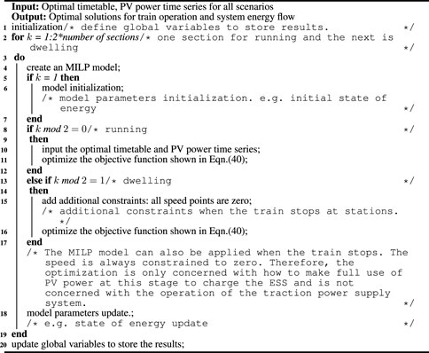
Step 2 is to optimize the train operation and energy flow management for the entire line through the MILP model for all inter-station segments. The basic structure of the MILP model has been provided in Section 2. Step 2 is to apply this MILP model to all inter-station operations. Therefore, the solutions of Step 2 are obtained by solving MILP models of different inter-station operations respectively and connecting them in sequence. The differences for the models are different starting and ending position and the operation time for different inter-station operations. The optimal timetable obtained by step 1, PV power, altitude, and the speed limit are the model input. The algorithm of step 2 is shown in Algorithm 2.

Algorithm 2. Step 2 Optimization: train operation and energy management optimization.

3.4 Model solving and algorithm evaluation

All the results in this paper are obtained by Gurobi academic solver version 9.1.2 on a computer with CPU of Intel(R) Core(TM) I3-7100U @ 2.40 GHz. To reduce the computational complexity, a two-step approach is proposed to decompose large-scale problems, and the nonlinear constraints are linearized by the PWL technique.

For step 1 optimization, the problem size is approximately 85 rows and 42 columns, with 189 non-zero variables, 42 continuous variables and 21 bilinear constraints. The decision variables related to speed, acceleration, force, and energy are continuous. The binary variables related to energy flow control and the variables related to PWL are integer. The solving time is about one minute. For step 2 optimization, each inter-station operation problem is a MILP model with a scale of about 135 rows and 3370 columns, 11,724 nonzero variables, 3427 continuous variables, 60 binary variables, and 95 SOS constraints. The solving time of each inter-station operation ranges from second-level to minute-level.

It should be noted that in the MILP model, two types of variables are linearized by the PWL technique. The first type is the speed-related nonlinear term, and the second type is the altitude and speed limit related to distance. It should be pointed out that the second type is necessary because the model proposed in this paper is based on time, while the actual altitude and the speed limit are nonlinear functions related to distance. The corresponding relationship between time, altitude and speed limit needs to be established through PWL. To illustrate the effectiveness of the PWL of speed-related nonlinear terms to reduce problem complexity without significantly sacrificing accuracy, the results of step 2 optimization of the MILP model and the mixed-integer nonlinear programming (MINLP) model without PWL processing on speed-related nonlinear terms were compared. The difference between MILP and MINLP model is that the MINLP model does not introduce SOS2 variables alpha and beta mentioned above, and directly takes the speed-related nonlinear terms as decision variables of the model. Numerical experiments show that there is only a 0.33% difference in the energy consumption of the step 2 optimization (733.37 MJ for the MILP model and 730.95 MJ for the MINLP model). However, the average solving time of the MILP model is reduced to 9.53% of the MINLP model (149.4 s for the MILP model and 1567.8 s for the MINLP model), which significantly improves the computational efficiency.

In summary, there are two types of PWL in the modeling, namely, the PWL of speed-related nonlinear terms and the PWL of distance-related altitude and speed limit. The PWL of the speed-related nonlinear term significantly improves the computational efficiency without sacrificing accuracy, and the PWL of the distance-related altitude and speed limit achieves the distance-time correspondence in the time-based model, thus allowing the spatial constraints to be considered in the time-based model.

4 Case studies

The data for the following cases including railway line data such as the length, altitude, speed limit, and operation data including timetable, time window, dwelling time all come from Qingdao Metro Line 11. The raw data and source code can be found in the Supplementary Materials S1. The length of Line 11 is 58.35 km and the total operation time including the dwelling is about 1 h. The first train leaves at 06: 15 and the last train leaves at 22: 00 in 1 day. It can be seen that the operation time includes zero PV power generation time periods in the morning and at night. Therefore, the following case analysis is divided into two parts: without PV power (4.1) and with PV power (4.2). The results for no PV power are used to simulate very low PV power in the morning and night.

Historical PV power data is from (Networks, 2014). Sixty days of data from June 11 to August 10 is used to cluster and generate three hypothetical weather types. All 60-days data is presented in Figure 4A. K-means method is used to implement the clustering (Thomas et al., 2017). The multi-day PV power data in the same cluster at 1 day’s same moment are averaged, resulting in one curve, which is considered to be the average level of PV power for that cluster. The number of clusters is chosen as three, which is commonly used as the number of weather classification and can roughly meet the needs of the forecast (Jie et al., 2015; Zhang et al., 2019). This number should be selected considering the balance between accuracy and model complexity, also considering the level of weather forecasts that can be achieved in reality. The clustering results are shown in Figure 4B.

FIGURE 4

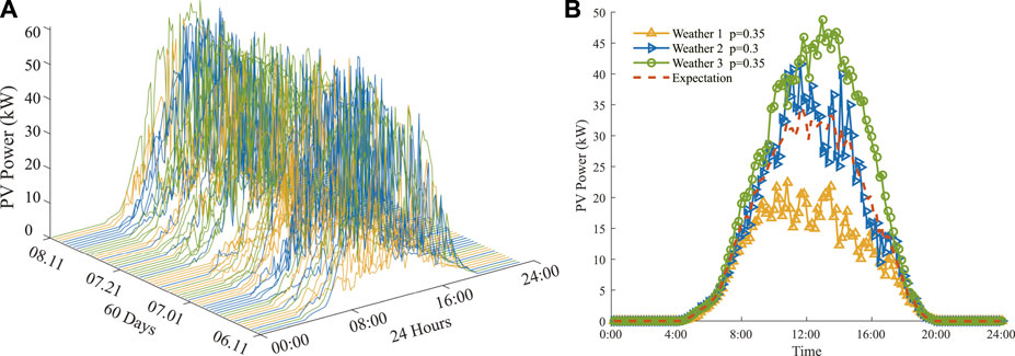
FIGURE 4. (A) Historical data of PV power in sixty consecutive days. (B) The average power of PV power generation after clustering.

4.1 Under the scenario without PV power

This case is designed to simulate the train operation in the morning and evening when the PV power is very low. The PV input to the model is always zero. In addition, since the stochastic PV power is not involved, this case can independently verify the effectiveness of the proposed two-step approach.

The time table comparison between the original timetable (MILP model) and the optimized timetable (two-step model) are shown in Figure 5A. The lengths of time windows are all 12 s, namely ±6 s from the original timetable. The behavior of the ESS and optimal speed trajectory are shown in Figure 6.

FIGURE 5

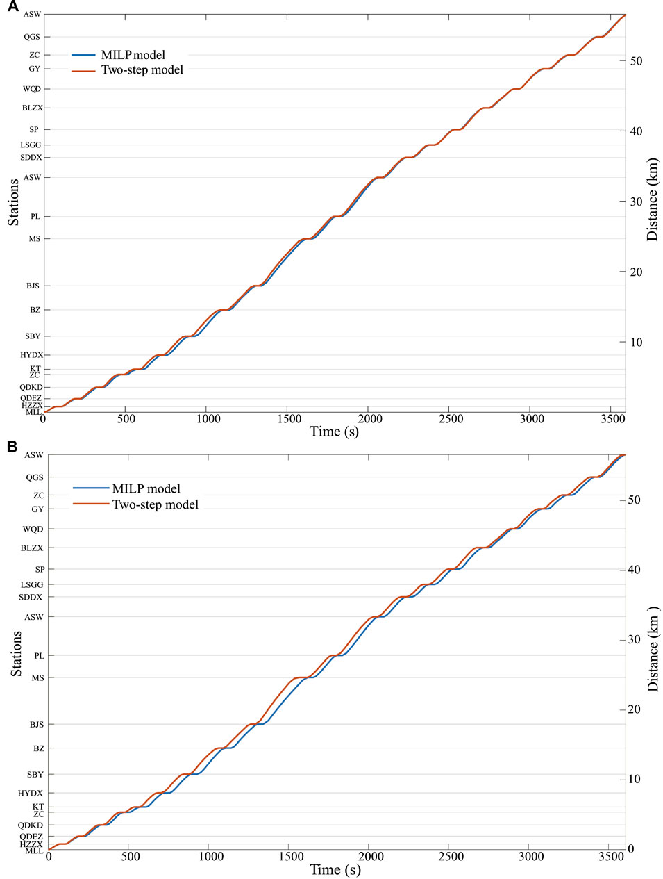
FIGURE 5. Comparison of the timetable obtained from the MILP model and the two-step model. (A) Under the scenario with no PV power. (B) Under the scenario with PV power, stochastic optimization results.

FIGURE 6

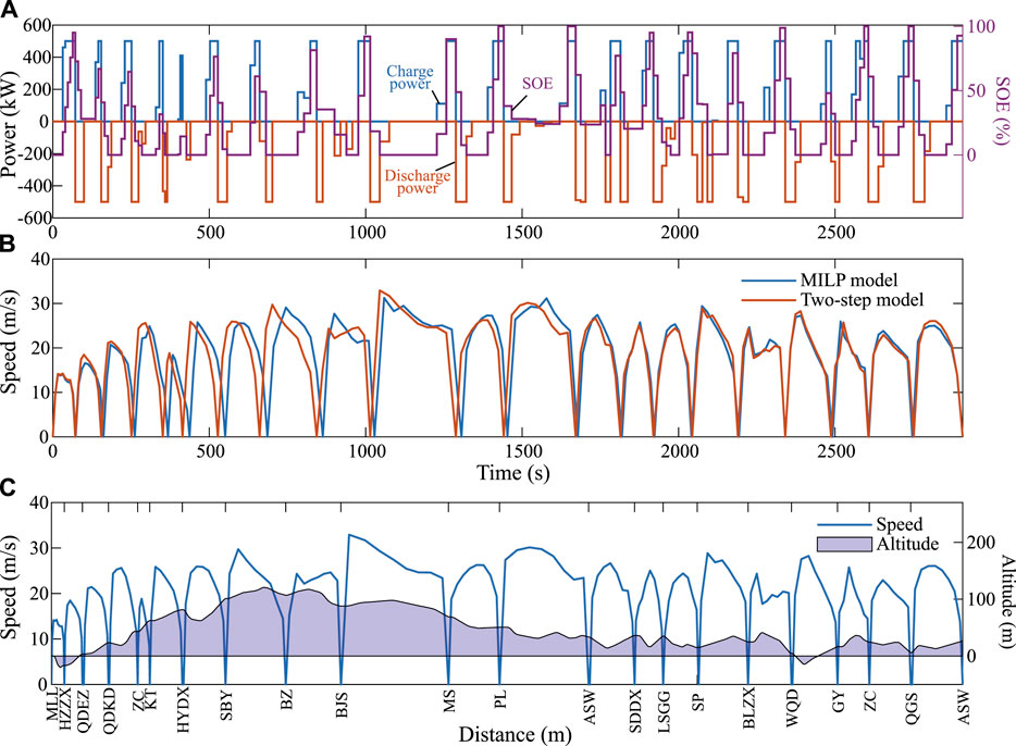
FIGURE 6. (A) Optimized charge and discharge strategy and SOE of the ESS obtained from the two-step model. (B) Comparison of speed trajectory between the MILP model and the two-step model. (C) Optimal speed trajectory and altitude for the whole line obtained from the two-step model.

Through Figure 5A, we observe that the optimized result allocates operation time for each section with total run time and time window constraints. Figure 6C shows the distance-based station distribution and the optimal speed trajectory of the whole line. Figure 6B shows the comparison of the speed trajectory under two control strategies. In the following case studies, the term “MILP model” refers to the speed trajectory and corresponding control strategy obtained from the MILP model on the original timetable. The term “two-step model” refers to the results of collaborative optimization of timetable and speed trajectory by the proposed two-step approach. Figure 6A shows the performance of the ESS corresponding to the results of the two-step model, including the charging and discharging power and the state of energy. It should be noted that due to the absence of PV input in this case, the system state does not change during the dwelling time. Therefore, the dwelling time is omitted in this Figure.

Figure 6B indicates that the two-step optimization approach coordinating the timetable and speed trajectory leads to changes on the timetable and speed. The energy consumption impact brought by these two different operations is that for the result optimized by MILP using the original timetable, the net energy consumption is 883.73 MJ. It is reduced by 3.2% through the proposed two-step approach, whose net energy consumption is 855.85 MJ.

It can be observed from Figure 6A that the ESS provides energy when the train is in the traction phase, and the state of energy decreases. The regenerative braking energy is recovered in the braking stage, and the state of energy increases.

This case verifies the effectiveness of the proposed two-step optimization approach in the condition without PV power generation and shows that the energy consumption can be further reduced by collaborative optimization of timetable and train speed trajectory than by simply optimizing speed trajectory.

4.2 Under the scenario with PV power

In this section, we assume that the train runs between 11:30 and 12:30, and the corresponding PV power data between this time interval shown in Figure 4B is selected as the input. The data points with markers are the real PV power data points. For the intervals in which the exact PV power is not available, linear interpolation is used to approximate. Therefore, the three lines in Figure 4B representing three generated weather types are regarded as PV power of three scenarios. It should be emphasized that all the following comparisons of energy consumption results for different models are based on the same PV condition. For this reason, the difference in energy consumption only comes from different models, rather than different PV power inputs. On this basis, the smaller net energy consumption means better model performance. Two subcases are considered, where the first subcase assumes that the weather forecast information cannot be obtained. In this case, we will obtain only one set of energy-efficient operation and control strategies through the two-step stochastic optimization. So that when running according to this strategy, the expectation of future energy consumption is minimal. But the actual energy-saving effect of each day depends on the presence of specific weather. The results of this situation are shown in the first following Subsection 4.2.1. In the second subcase, it is assumed that the weather type information can be obtained. We can further classify the weather and conduct the two-step approach under different weather types to obtain energy-efficient operation and control strategies. In the following description, the term “weather-type-based two-step model” refers to the two-step approach according to the corresponding weather type. The results are shown in the second Subsection 4.2.2.

Then, Monte Carlo simulations of different operation strategies are carried out for sixty consecutive days. The results obtained from three models, i.e. MILP model, two-step model, and weather-type-based two-step model are compared to verify the model’s effectiveness. The results are shown in 4.2.3.

4.2.1 Forecast information about weather types is unavailable

In this section, we assume that any forecast information about future weather conditions cannot be obtained and only historical PV power data are available. We cluster the data to generate three scenarios with different probabilities as the input of two-step stochastic optimization model. The comparison between the timetable obtained by the two-step model and the MILP model is presented in Figure 5B. The speed trajectory, state of energy, and PV power distribution strategy under the same PV power output condition for the MILP model and the two-step model are shown in Figure 7. It is worth mentioning that there is no energy exchange with the train traction power supply system when the train stops at the station, but the energy of the PV power generation system can be recovered by the ESS. Therefore, there may still be changes in the state of energy, which is reflected in Figure 7C. Table 3 lists the comparison of indicators for each system. From the perspective of total energy consumption, the two-step model reduces the net energy consumption by 2.57% compared with the result of the MILP model, which indicates the validity of the proposed two-step model.

FIGURE 7

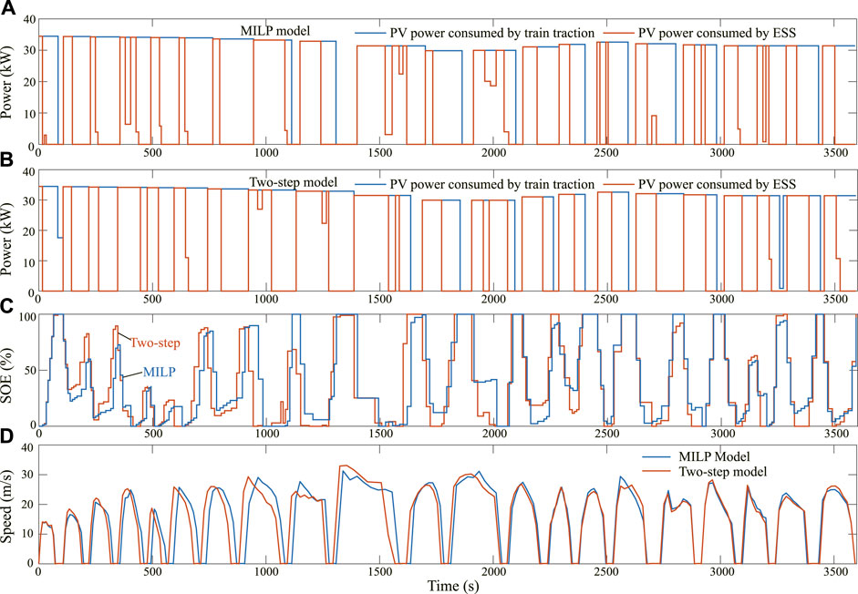
FIGURE 7. (A) PV power distribution strategy of the MILP model. (B) PV power distribution strategy of the two-step model. (C) SOE comparison between the MILP model and the two-step model. (D) Speed trajectory comparison between the MILP model and the two-step model.

TABLE 3

TABLE 3. The performance of each system for the MILP model and the two-step model.

Since there is no initial energy in the ESS and the energy is recovered and released repeatedly by the ESS during the entire process. Therefore, the total discharge energy of the ESS represents the potential of the buffer capacity. The larger this value represents that the ESS plays a greater role in the supply of insufficient energy and the absorption of additional energy. It is noted that this indicator is increased by 5.18% by the two-step model, which implies that the proposed two-step stochastic optimization adjusts timetables and train control strategies to make it more conducive to the greater role of the ESS, thereby reducing net energy consumption.

4.2.2 Forecast information about weather types is available

In this section, we assume that the weather type information can be predicted. A comparison between the results obtained by two-step approach and those obtained by weather-type-based two-step model is conducted. Specifically, the historical PV power data are clustered to obtain three scenarios, as mentioned above. The weather-type-based two-step model is executed to obtain corresponding optimal strategies. In order to evaluate the performance of two-step model under various weather types, we operate the strategy obtained by the two-step model in a specific weather type to simulate the train operates according to the two-step stochastic optimization result when this weather occurs in the future. The energy consumption comparison between results obtained by two-step model and weather-type-based two-step model is tabulated in Table 4. The corresponding speed trajectories are shown in Figure 8.

FIGURE 8

FIGURE 8. The comparison between the optimal speed trajectory obtained from the weather-type-based two-step model under different weather types and the MILP model.

TABLE 4

TABLE 4. Energy-saving performance when various weather conditions occur for the two-step model and the weather-type-based two-step model.

The results show that when the three scenarios appear, the net energy consumption of the results obtained by the two-step model is 0.47%, 2.4%, and 2.0% higher than that obtained by the weather-type-based two step model, respectively. The results indicate that optimization according to weather classification and prediction has the potential to further reduce the net energy consumption. On the other hand, it also means that more forecast information is needed, and the train operation strategy needs to be more frequently adjusted, bringing more costs and challenges to practical applications.

4.2.3 Long-term operation monte carlo simulation

For trains operating from 11: 30 to 12: 30, the Monte Carlo simulation for sixty consecutive days is conducted to verify the effectiveness and robustness of the proposed two-step stochastic optimization model. The following three control strategies are used for comparison, which are the MILP model, the two-step model, and the weather-type-based two step model assuming that the weather type can be predicted. The net energy consumption of the three operation strategies for sixty consecutive days is shown in Figure 9. The total energy consumption is listed in Table 5.

FIGURE 9

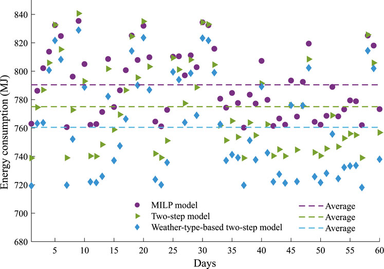
FIGURE 9. Energy consumption comparison of Monte Carlo simulation for 60-days results of three operation strategies.

TABLE 5

TABLE 5. Energy consumption comparison of Monte Carlo simulation with different optimization strategies for sixty consecutive days.

It can be seen from Figure 9 that the net energy consumption of each day’s optimization results based on weather classification is always the lowest. This means a better energy-saving effect can be achieved by considering the weather type, which indicates the importance of incorporating PV power information into the optimization model. The results of two-step model are better than the MILP model most of the time. However, it may also be worse depending on the specific condition due to the stochastic characteristic. On the whole, the proposed two-step stochastic optimization can achieve 1.95% energy consumption reduction.

The results show that the two-step optimization approach proposed in this study considering the stochastic PV power optimizes the timetable, speed trajectory, and energy management strategy collaboratively. It can achieve energy-saving in long-term operation compared with the control strategy obtained by only speed trajectory optimization. The energy consumption can be further reduced if the weather types are further considered in the optimization.

5 Conclusion

In this study, a two-step stochastic optimization is proposed to solve the long-term energy-efficient operation and energy management problem of the train traction power supply system integrated with the PV power system and the ESS. The proposed curve fitting method can estimate the inter-station energy consumption as an explicit function of operating time and PV power accurately. Then, the problem of minimizing the net energy consumption of the whole line is converted to minimizing the sum of all the inter-station energy consumption, which reduces the computational complexity. The proposed two-step stochastic optimization can realize the coordination of the timetable, train operation control, and energy management, bringing a better energy-saving effect. The results show the effectiveness of the model under both with and without PV power conditions. The Monte Carlo simulation is conducted for sixty consecutive days to compare the energy consumption for three operation strategies, which are the proposed two-step stochastic optimization, MILP using the original timetable, and two-step optimization considering the weather type classification. The results demonstrate the potential of the proposed two-step stochastic optimization in reducing the net energy consumption of the integrated system for a long-term operation. Additionally, a better energy-saving effect can be achieved if combined with the weather information. Selecting a reasonable number of scenarios to characterize the stochastic power of the PV system can achieve the balance of model complexity, energy-saving effect, PV power prediction cost, and industrial practicability.

For future work, weather types will be more rigorously classified, and a larger amount of PV power data under specific weather types will be extracted to obtain scenarios that can more accurately characterize the actual situation. The relationship between scenario number and model complexity and net energy consumption will be explored to suggest a more reasonable scenario number.

Data availability statement

The original contributions presented in the study are included in the article/supplementary material, further inquiries can be directed to the corresponding authors.

Author contributions

JL, MF, SL, CW designed the research framework and organized the paper structure. JL contributed to the case study design, implementation, and figure drawing. JL wrote the first draft of the manuscript. MF, SL, CW provide detailed suggestions for research and the article. All authors contributed to manuscript revision, read, and approved the submitted version.

Funding

This research is supported in part by the 2022 Fundamental and Applied Fundamental Research Project of Guangzhou Basic Research Program, in part by Featured Innovation Project of the Department of Education of Guangdong Province (NO.2021KTSCX001) and in part by the Fundamental Research Funds for the Central Universities (NO.2020ZYGXZR087).

Acknowledgments

Thanks to all the members who worked hard on this project, and thanks to Shien-Ming Wu School of Intelligent Engineering for providing a good scientific research environment.

Conflict of interest

The authors declare that the research was conducted in the absence of any commercial or financial relationships that could be construed as a potential conflict of interest.

Publisher’s note

All claims expressed in this article are solely those of the authors and do not necessarily represent those of their affiliated organizations, or those of the publisher, the editors and the reviewers. Any product that may be evaluated in this article, or claim that may be made by its manufacturer, is not guaranteed or endorsed by the publisher.

Supplementary Material

The Supplementary Material for this article can be found online at: https://www.frontiersin.org/articles/10.3389/fenrg.2022.957891/full#supplementary-material

References

Aguado, J. A., Sánchez Racero, A. J., and de la Torre, S. (2018). Optimal operation of electric railways with renewable energy and electric storage systems. IEEE Trans. Smart Grid 9, 993–1001. doi:10.1109/TSG.2016.2574200

CrossRef Full Text | Google Scholar

Ehteshami, H., Hashemi-Dezaki, H., and Javadi, S. (2022). Optimal stochastic energy management of electrical railway systems considering renewable energy resources’ uncertainties and interactions with utility grid. Energy Sci. Eng. 10, 578–599. doi:10.1002/ese3.1053

CrossRef Full Text | Google Scholar

González-Gil, A., Palacin, R., Batty, P., and Powell, J. (2014). A systems approach to reduce urban rail energy consumption. Energy Convers. Manag. 80, 509–524. doi:10.1016/j.enconman.2014.01.060

CrossRef Full Text | Google Scholar

Guo, X., Sun, H., Wu, J., Jin, J., Zhou, J., and Gao, Z. (2017). Multiperiod-based timetable optimization for metro transit networks. Transp. Res. Part B Methodol. 96, 46–67. doi:10.1016/j.trb.2016.11.005

CrossRef Full Text | Google Scholar

Huang, Y., Yang, L., Tang, T., Gao, Z., Cao, F., and Li, K. (2018). Train speed profile optimization with on-board energy storage devices: A dynamic programming based approach. Comput. Industrial Eng. 126, 149–164. doi:10.1016/j.cie.2018.09.024

CrossRef Full Text | Google Scholar

Jie, S., Lee, W. J., Liu, Y., Yang, Y., and Peng, W. (2015). Forecasting power output of photovoltaic systems based on weather classification and support vector machines. IEEE Trans. Ind. Appl. 48, 1064–1069. doi:10.1109/tia.2012.2190816

CrossRef Full Text | Google Scholar

Kaffash, M., Bruninx, K., and Deconinck, G. (2021). Data-driven forecasting of local pv generation for stochastic pv-battery system management. Int. J. Energy Res. 45, 15962–15979. doi:10.1002/er.6826

CrossRef Full Text | Google Scholar

Kanchev, H., Colas, F., Lazarov, V., and Francois, B. (2014). Emission reduction and economical optimization of an urban microgrid operation including dispatched pv-based active generators. IEEE Trans. Sustain. Energy 5, 1397–1405. doi:10.1109/TSTE.2014.2331712

CrossRef Full Text | Google Scholar

Liu, P., Yang, L., Gao, Z., Huang, Y., Li, S., and Gao, Y. (2018). Energy-efficient train timetable optimization in the subway system with energy storage devices. IEEE Trans. Intell. Transp. Syst. 19, 3947–3963. doi:10.1109/tits.2018.2789910

CrossRef Full Text | Google Scholar

Lu, S., Hillmansen, S., Ho, T. K., and Roberts, C. (2013). Single-train trajectory optimization. IEEE Trans. Intell. Transp. Syst. 14, 743–750. doi:10.1109/tits.2012.2234118

CrossRef Full Text | Google Scholar

Montrone, T., Pellegrini, P., and Nobili, P. (2018). Real-time energy consumption minimization in railway networks. Transp. Res. Part D Transp. Environ. 65, 524–539. doi:10.1016/j.trd.2018.09.018

CrossRef Full Text | Google Scholar

Networks, U. P. (2014). Photovoltaic (pv) solar panel energy generation data – London datastore. Available at: https://data.london.gov.uk/dataset/photovoltaic--pv--solar-panel-energy-generation-data/(Accessed April 27, 2022).

Google Scholar

Park, S., and Salkuti, S. R. (2019). Optimal energy management of railroad electrical systems with renewable energy and energy storage systems. Sustainability 11, 6293. doi:10.3390/su11226293

CrossRef Full Text | Google Scholar

Scheepmaker, G. M., Goverde, R. M., and Kroon, L. G. (2017). Review of energy-efficient train control and timetabling. Eur. J. Operational Res. 257, 355–376. doi:10.1016/j.ejor.2016.09.044

CrossRef Full Text | Google Scholar

Şengör, İ., Kılıçkıran, H. C., Akdemir, H., Kekezoǧlu, B., Erdinc, O., and Catalao, J. P. (2017). Energy management of a smart railway station considering regenerative braking and stochastic behaviour of ess and pv generation. IEEE Trans. Sustain. Energy 9, 1041–1050. doi:10.1109/tste.2017.2759105

CrossRef Full Text | Google Scholar

Shen, X., Wei, H., and Wei, L. (2020). Study of trackside photovoltaic power integration into the traction power system of suburban elevated urban rail transit line. Appl. Energy 260, 114177. doi:10.1016/j.apenergy.2019.114177

CrossRef Full Text | Google Scholar

Su, S., Li, X., Tang, T., and Gao, Z. (2013). A subway train timetable optimization approach based on energy-efficient operation strategy. IEEE Trans. Intell. Transp. Syst. 14, 883–893. doi:10.1109/tits.2013.2244885

CrossRef Full Text | Google Scholar

Thomas, D., Deblecker, O., and Ioakimidis, C. S. (2017). Optimal operation of an energy management system for a grid-connected smart building considering photovoltaics’ uncertainty and stochastic electric vehicles’ driving schedule. Appl. Energy 210, 1188–1206. doi:10.1016/j.apenergy.2017.07.035

CrossRef Full Text | Google Scholar

Wang, X., Tang, T., Su, S., Yin, J., Gao, Z., and Lv, N. (2021). An integrated energy-efficient train operation approach based on the space-time-speed network methodology. Transp. Res. Part E Logist. Transp. Rev. 150, 102323. doi:10.1016/j.tre.2021.102323

CrossRef Full Text | Google Scholar

Wu, C., Lu, S., Xue, F., Jiang, L., Chen, M., and Yang, J. (2021). A two-step method for energy-efficient train operation, timetabling, and onboard energy storage device management. IEEE Trans. Transp. Electrific. 7, 1822–1833. doi:10.1109/tte.2021.3059111

CrossRef Full Text | Google Scholar

Wu, C., Zhang, W., Lu, S., Tan, Z., Xue, F., and Yang, J. (2019). Train speed trajectory optimization with on-board energy storage device. IEEE Trans. Intell. Transp. Syst. 20, 4092–4102. doi:10.1109/TITS.2018.2881156

CrossRef Full Text | Google Scholar

Zhang, X., Fang, F., and Liu, J. (2019). Weather-classification-mars-based photovoltaic power forecasting for energy imbalance market. IEEE Trans. Ind. Electron. 66, 8692–8702. doi:10.1109/tie.2018.2889611

CrossRef Full Text | Google Scholar