Numerical simulation based on a weakly compressible model in the multi-elbow pipe

The negative pressure wave method is a more important method used for pipeline leak detection and location in practical engineering applications. In this paper, a new method based on a weakly compressible model and a standard k-e turbulence model is proposed, which is used to simulate the propagation of negative pressure waves in pipelines. The purpose of the study is to capture the negative pressure wave propagation phenomenon in multi-elbow pipe leaks based on the weakly compressible method and to investigate the negative pressure wave propagation law in multi-elbow pipes. The results show that the negative pressure wave transmission phenomenon inside the leaking pipeline can be calculated by using the weakly compressible model, and the transmission law is consistent with the actual one. It was found that the propagation velocity of the negative pressure wave in the elbow was 1.4% higher than that in the straight pipe, and there was backflow in each elbow, which affected the propagation distance of the negative pressure wave at different locations in the elbow. The vortex viscosity and turbulence frequency in the axis of the elbow were 12.2% and 5.4% higher than those in the straight pipe, respectively. In addition, the high viscous force and pulsation frequency in the elbow accelerate the volume compression and expansion of the flow elements, for which the equivalent length equation of the elbow in the negative pressure wave leakage localization method is proposed to verify the applicability of the weakly compressible model. The research in this paper reveals the internal effects of the negative pressure wave method in the bend as well as provides an innovative equivalence formula for the negative pressure wave leak location method. This work will provide a more accurate method for pipeline leak detection and localization.

Introduction

The property of unintentional release of fluid in a pipe is called leakage. Pipeline leakage may be caused by human factors or others, such as sudden changes in pipeline pressure, corrosion of fluid to pipe, impact of foreign objects on the pipe, defects of the pipe material, lack of pipeline maintenance. In most cases, the occurrence of a leak can be harmful and even cause some serious problems. Hence, it is pretty important to detect the leak quickly and locate the leak accurately, and then carry out emergency repairs to save energy and protect the environment.

In the automatic monitoring system of pipeline, the methods of pipeline leakage detection are roughly divided into three categories. The first type of category is mainly to detect leaks by directly measuring some variables in the pipe, such as inlet flow, outlet flow, pressure and temperature. The second type of category mainly selects some unmeasured quantities, such as internal state variables, model parameters and feature quantities of pipeline systems. The third type of category is also most commonly used recently, combined with flow field variables and signal processing techniques. For instance, the negative pressure wave method. Huang et al. (2021) reported detailed experimental work on field testing techniques for pipeline leak detection using a spherical leak detector with acoustic measurements. In order to break through the limitation that acoustic testing can only be performed on small diameter pipes, Mergelas and Henrich (2005) have improved this leak detection method. Different from the previous one, the new method relies on acoustic sensors inside the pipeline to detect leakage noise signals. A major challenge is that acoustic signals are hard to detect sensitively. Using the data measured by the pressure sensor, velocity sensor and acceleration sensor, Gao et al. (2005) studied the cross-correlation characteristics of the leakage signal, and proved that it is feasible to measure the pressure signal with low SNR using the hydrophone. Due to the problem of accelerometer measurement in peak value of correlation coefficient and signal delay, Willsky (1976) have respectively proposed the use of state variable method and parameter identification method to detect pipeline leakage, which establish a strong foundation for the later combination of these two methods in practical projects.

Besides the above two types of methods, there are some other related methods for detecting pipeline leaks. In order to solve the leakage problem in a specific environment, Lee et al. (2001) developed a ceramic-based humidity sensor in which a local humidity detection method was used. And it basically met the requirements of the pipeline leak detection system. Since then people are no longer satisfied with the requirements of leak detection, and the reliability and accuracy of detection in the pipeline systems are particularly important. Ferrante and Brunone (2003) used the impulse response method to obtain an analytical expression of the negative pressure head spectrum in transients downstream and at the cross section of a single pipe. By analyzing the pressure harmonic diagram in the transient process, namely, comparing the pressure changes before and after, he proposed a diagnostic tool that can be used to evaluate the reliability of the pipeline system. Verde et al. (2007) proposed a method for identifying the properties of pressure signals in a pipeline, based on a combination of transient and steady state, and could identify the relevant unknown parameters of multiple leaks in the pipeline offline. The method widely used for pipeline leak detection is called the negative pressure wave method by Zhang et al. (2014). In order to solve the delay problem of negative pressure wave method in detecting micro-leakage, they proposed the LDMS method based on dynamic pressure sensor, and it reduce the delay time and improve the sensitivity and resolution effectively. Ming and Zhao (2012) used CFD software FLUENT to simulate the effects of four different grid numbers on the internal flow conditions in a three-way pipe under two different turbulence models. The results show that when the grid number reaches more than 1.2 million, the increase of grid number will no longer affect the temperature and velocity of the fluid. Meanwhile, the LES model simulation yields clearer results for the interior of the pipe than those obtained by the RANS model simulation.

In a more recent study, Ben-Mansour et al. (2012) simulate the flow around different leakage holes under steady and transient state. The results show that when the leakage is small, it will not cause too much pressure fluctuation, but it will cause the amplitude and frequency of the pressure signal spectrum to increase. Wang (2000) studied the propagation and attenuation of pressure waves in the bend in detail through experiments. The results show that the propagation of pressure wave in the bend is quite different from that in the straight pipe. The pressure on the outside of the bend is obviously larger than that on the inside, and it will decay quickly after passing through the bend. Liu and Qu (1998) derived from the dispersion equation of harmonic circular cycle in curved pipe. In a bend, multiple reflections may occur so that the pressure waves between the inner surface and the outer surface can travel in a circular direction. Qi et al. (2016) used the finite element method to simulate the propagation of guided waves in the bend. The results show that the velocity of guided waves through the bend is closely related to the excitation frequency. The difference between a bend and a straight pipe is that a bend has a finite radius of curvature. In fact, when the curvature radius of the bend becomes infinite, the bend can be considered a straight pipe. This conjecture has been verified numerically in this paper.

In summary, the above-mentioned studies indicate that in a simple structure with multiple elbows, the standard k-e turbulence model can be used to simulate leakage in the pipeline. However, when the pipeline leaks, the local pressure at the leak point suddenly decreases, and the phenomenon of negative pressure wave propagation and its influence on the internal of the pipeline are still lacking research. In addition, the numerical simulation of the transmission process of negative pressure waves and the transmission characteristics of negative pressure waves in multi-elbow pipelines are also a relatively new study direction.

In this paper, by considering the variation of inlet pressure at the time of leakage, we propose and discuss transmission characteristics of negative pressure wave based on a weakly compressible method and its prediction method. The main objectives of this research are: Equation 1 to capture the negative pressure wave propagation phenomenon in multi-elbow pipeline leakage based on weakly compressible method, Eq. 2 to analyze the difference and the underlying cause of negative pressure wave propagation characteristics in elbows and straight pipes, and finally to predict the negative pressure wave propagation law in the multi-elbow pipe. In this work a new, the propagation of negative pressure waves was successfully simulated and monitored using a weakly compressible model, and various flow characteristics of the negative pressure wave phenomenon were obtained. By analyzing the information of the internal flow field variables in the multi-elbow pipeline, a reasonable explanation is found for the similar transfer velocity difference phenomenon between straight and elbow pipes, and a formula for the equivalent length of the elbow in the negative pressure wave leakage localization method is given. This result provides a new idea and a complete formula basis for the calculation of actual pipeline leakage cases.

Computational details and geometric model

Numerical modeling and computational set-up

For unsteady compressible turbulent flows, the conservation laws of mass and momentum are written as:

Continuity equation:

$\frac{\partial \rho }{\partial t}+\frac{\partial }{\partial x_j}\left(\rho U_j\right)=0.(1)$

Momentum equation:

$\frac{\partial }{\partial t}\left(\rho U_i\right)+\frac{\partial }{\partial x_j}\left(\rho U_i{U}_j\right)=-\frac{\partial p}{\partial x_i}+\frac{\partial }{\partial x_j}\left(\mu \frac{\partial U_i}{\partial x_i}-\rho \overline{u_i{u}_j}\right),(2)$

Where U_i is the velocity vector, p is the pressure, ρ is the density, and μ is the dynamic viscosity. The additional Reynolds stress term ($-\rho \overline{u_i{u}_j}$) is modelled by turbulence models.

The increase in the fluid temperature during the process is assumed to be insignificant, and thus the solution to the energy equation is not necessary. In order to consider the compressibility effects under isothermal conditions, the density variation is taken into account by coupling density and pressure (Raisee Dehkordi, 1999):

$dpd\rho =K_f\rho ,(3)$

Where K_f is the bulk modulus of elasticity of the fluid, which is assumed to be independent of temperature, and thus the density is just the function of the pressure. (Korteweg, 1878)

Because the above relationship ignores pipe elasticity, applying it to negative pressure wave simulations results in an overestimation of wave velocity, resulting in pressure rises greater than those observed in tests. In order to solve this problem, the bulk modulus in this study has been changed to:

$K_f^{\prime }=K_f\left(1+K_{f}DeE\right),(4)$

where E is the pipe Young’s modulus, e is the pipe thickness, and D is the pipe diameter.

The above correction now takes into account both the fluid compressibility and the elasticity of the pipe. Consequently, the wave velocity decreases from$a=\sqrt{K_f/\rho }$to$a^{\prime }=\sqrt{K_f^{\prime }/\rho }$, resulting in pressure variation identical to the experimental observations (Dou et al., 1997).

As commented above, some earlier weakly compressible simulations indicated that the k-e turbulence model can produce reasonable pressure variations. Furthermore, it performs well in simulating the flow at the leak. Because of its wide application range, economical calculation cost, and reasonable accuracy, it has better applicable conditions in pipeline leakage flow. Therefore, in the current study, the standard k-e turbulence model was adopted to simulate turbulent negative pressure waves. The unknown Reynolds stress tensor of the Navier-Stokes equation in the model is obtained by Boussinesq approximation (SaemI et al., 2019).

In this study, the SIMPLE algorithm is used to determine the pressure field, and the nonlinear convective term in all transport equations is approximated using the second-order upwind scheme. In addition, a first-order implicit scheme is used for the discretization of the time derivatives. The fluid medium is water and its density is compressible.

To simulate the negative pressure wave phenomenon, steady-state computations are first performed using the constant pressure-inlet and outflow. (Martins et al., 2016). This corresponds to the development of the normal flow of liquid in the pipeline. When the converged solution is reached, the simulations continue with the unsteady scheme. In the unsteady simulation, the value of the inlet pressure is reduced, and other boundary conditions are unchanged. At this point, it represents that the leak is occurring and the pressure at the leak point drops sharply.

Geometric model and convergence analysis

The numerical simulations are performed with 3D geometry. In addition, the outlet pipe is extended with sufficient length to prevent the effects of backflow, and we have eight pressure monitoring points in this multi-elbow pipe, as shown in Figure 1. In the Figure 1, where L₁ = 1000mm, L₂ = 400mm, L₃ = 500mm, L₄ = 2000mm, pipe diameter D = 150 mm and radius of curvature R_c = 250 mm.

FIGURE 1

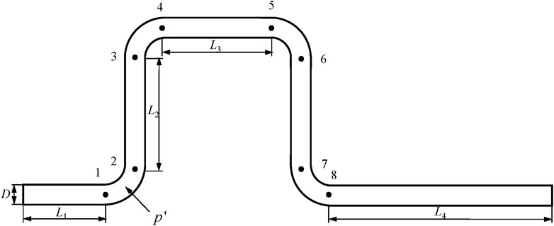
FIGURE 1. Multi-elbow pipeline for numerical simulation and its monitoring point arrangement.

The distribution of grid nodes in the pipe cross-section is shown in Figure 2A. As can be observed, a structured grid is used in the whole section of the pipeline, and the grid nodes are clustered near the pipe wall. For turbulent flow computations, the y + values of the nodes adjacent to all solid walls are kept close to unity, ensuring that the near-wall nodes are positioned within the viscous sub-layer. Figure 2B shows the computational grids used for the pipe in the 3D numerical simulations.

FIGURE 2

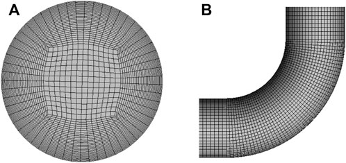
FIGURE 2. Pipe geometry: (A) Pipe cross-section mesh in 3D; (B) Local mesh of elbow.

It is necessary to verify the independence of the curved mesh. Generally speaking, if the geometric model is mesh-divided correctly, the turbulence simulation results based on Reynolds-Average Navier-Stokes will not show obvious fluctuation with the increase of the number of model grids. Therefore, four sets of grids with different total grid Numbers (a)2.8 million, (b)3.8 million, (c)4.8 million and (d)5.8 million, respectively) were used for stable numerical simulation under the condition of stable inlet pressure of elbow. The model simulation software is ANSYS FLUENT 18.0, the inlet condition is pressure inlet, the gauge total pressure is 300kPa, and the outlet condition is outflow. Figure 3 shows the four different dimensionless pressure pulsation coefficient C_p in the four grid groups. C_p is a measure of the degree of boundary layer flow separation and is defined as:

$C_p=\frac{P-\overline{P}}{\frac{1}{2}\rho u^2},(5)$

where P is the pressure at monitoring point one at different times, $\overline{P}$is the average pressure, ρ takes the density of liquid water, u takes the velocity of monitoring point 1. The results show that all the deviations are within 0.5%. Considering saving computing time and resources, the second grid b was selected.

FIGURE 3

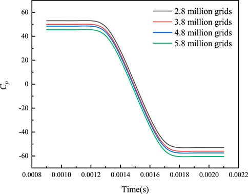
FIGURE 3. Grid independence check for the simulation.

Results and discussion

The phenomenon of negative pressure wave propagation

Figures 4A–C shows the comparison of negative pressure wave propagation in monitoring points of inlet and outlet in the same elbow. In these figures, it can be clearly seen that transmission of the negative pressure wave is occurring in the pipeline. The transmission curve of the negative pressure wave has a significant time difference between the inlet and outlet of the elbow. We have sorted out the time when the negative pressure wave passes through the different elbow’s inlet and outlet positions. We default to calculate velocity is the length of the elbow axis divided by the corresponding time difference between inlet and outlet.

FIGURE 4

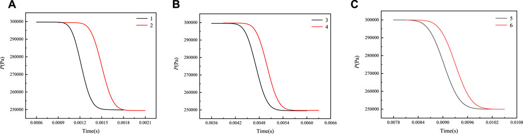
FIGURE 4. Comparison of negative pressure wave propagation in monitoring points of inlet and outlet in the same elbow with 0.25 m curvature radius: (A) first elbow; (B) second elbow; (C) third elbow.

We get the time difference of negative pressure wave between the same elbow’s inlet and outlet by correlation analysis, and the value of time difference in the three elbows is the same. When the length of the center interface of the elbow is used as the distance, we can easily calculate the velocity of negative pressure waves.

As shown in Table 1, it is worth noting that the velocity of a negative pressure wave changes when it passes through elbows and straight pipes. The velocity values in the table are the time step of the negative pressure wave arriving at each monitoring point and the transfer velocity between adjacent monitoring points. The rule for calculating the transfer velocity is the ratio of the length of the central axis of the elbow to the time difference between the corresponding inlet and outlet. As the negative pressure wave passes through each elbow, its velocity is the same. However, the velocities of the P2-P3 and P4-P4 segments are also slightly different. This difference may be due to calculation errors caused by the different straight pipe lengths in the two sections. In addition, the velocity changes significantly when the negative pressure wave passes through an elbow and the straight pipe below it. The velocity is faster at the elbow, while it slows down when the wave passes through the straight pipeline.

TABLE 1

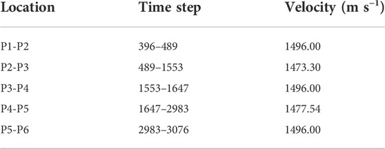
TABLE 1. Time step of pressure wave transmission at each monitoring point and calculation velocity of adjacent monitoring points.

Figure 5 shows the process of the negative pressure wave at different positions when passing the first elbow, where T₁ indicates the moment when the pressure wave just reaches the position in front of the elbow inlet, T₂, T₃, T₄, T₅ represent the moment respectively when the negative pressure wave reaches the position in the elbow at the angle of 0°, 30°, 60°, 90°, T₆ is the moment when the pressure wave reaches the position after the elbow exit.

FIGURE 5

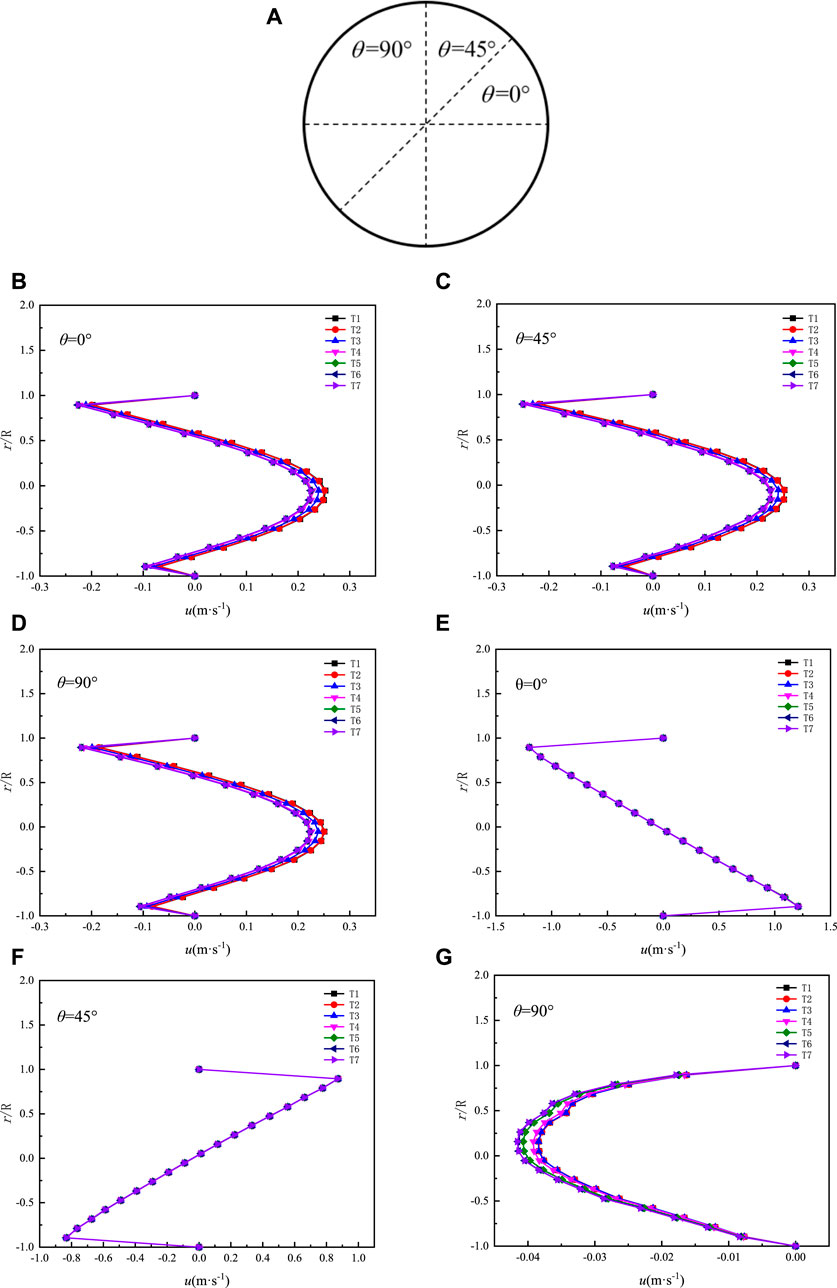
FIGURE 5. Flow velocity profile at the inlet and outlet of the first elbow:(A) Schematic view of the cross-section and the lines selected to represent the velocity profiles at entrance and exit of first elbow, (B–D) velocity profiles at entrance of first elbow at different selected angular positions in the pipe, (E–G) velocity profiles at exit of first elbow at different selected angular positions in the pipe.

The analysis on the phenomenon of negative pressure wave propagation

In order to explain those phenomena, we did some analysis of the flow inside the elbow. The streamwise velocity profiles on the inlet and outlet of the first elbow are displayed in Figure 5. Three different angles (θ = 0°, 45°, and 90°), shown in Figure 5A, are chosen to present the velocity profiles obtained from numerical simulation. The computed axial velocity profiles at the entrance at seven times instants, namely t = 6T, 7T, 8T, 9T, 10T, 11T, and 12T are presented in Figures 5B–D, where 6T = 0.0009 s represents the moment when the negative pressure wave arrived at the entrance of the elbow. Figures 5E–G shows the computed axial velocity profiles at the exit at seven times instants. It is observed that the elbow creates a non-symmetrical velocity field close to those regions. As the fluid develops in the elbow, the velocity distribution becomes more and more non-axisymmetric, and the reflux phenomenon occurs near the outside of the elbow.

In order to explore the reason for the different propagation velocity of negative pressure waves in curved and straight pipes, we set up a control group with the same bending angle (90°), the same elbow radius (0.075 m) and the different curvature radius (Ⅰ)0.25, (Ⅱ)0.3, (Ⅲ)0.35,and (Ⅳ)0.4 m, as shown in Table 2.

TABLE 2

TABLE 2. Comparison of the calculation velocity of adjacent monitoring points in four cases.

Figures 6A–C shows the negative pressure wave propagation situation in the first three elbows monitored at each monitoring point of the pipeline. The two curves in each picture represent the pressure waveforms of the elbow inlet and the pressure outlet respectively. It can be seen that we can still get the typical negative pressure wave propagation curve.

FIGURE 6

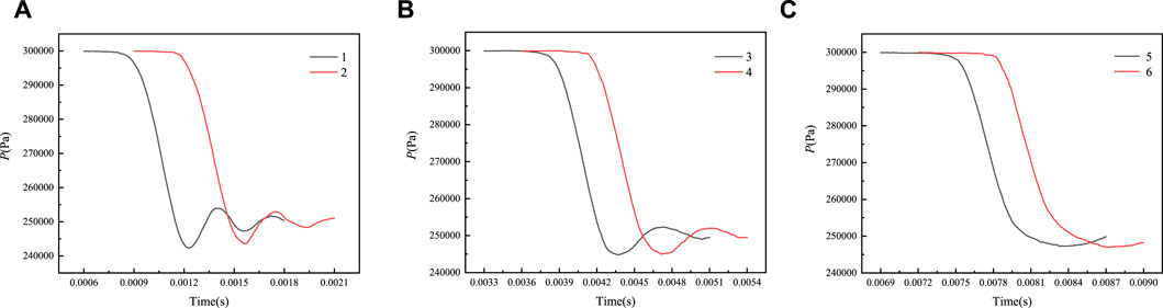
FIGURE 6. Comparison of negative pressure wave propagation in monitoring points of inlet and outlet in the same elbow with 0.3 m curvature radius: (A) first elbow, (B) second elbow (C) third elbow.

We adopt the correlation analysis on the four curves, and deal with the relative position of the falling edge of the two negative pressure waves, getting the time step difference between the inlet and outlet in the first elbow. According to this, we can also get the propagation time of the pressure wave in each following straight pipe and elbow. And we compared it with pipe mentioned above and listed the Table 2.

From Table 2, it can be seen that for four multi-bend pipes with different radii of curvature, the propagation law of the negative pressure wave shows similarity, that is, the propagation velocity of each bend section and straight section is approximately the same, and the propagation velocity in the bend section is slightly higher than that in the straight section.

To explain this phenomenon, we have drawn the development diagram of the corresponding position of the negative pressure wave’s front edge in different time steps when passing through the first elbow, as shown in Figure 7. It shows the process of the negative pressure wave at different positions when passing the first elbow, where T₁ indicates the moment when the pressure wave just reaches the position in front of the elbow inlet, T₂, T₃, T₄, T₅ representing the moment respectively when the negative pressure wave reaches the position in the elbow at the angle of 0°, 30°, 60° 90°, and T₆ is the moment when the pressure wave reaches the position after the elbow exit. It is not difficult to find out from the figure that when the negative pressure wave passes through the elbow, its front edge is not always perpendicular to the direction of propagation. In T₁ and T₂ moment, the negative pressure wave is transmitted from the straight pipe to the inlet of the elbow, and the front edge is perpendicular to the direction of propagation. From T₃ to T₆ the closer to the position of the outer pipe wall of the elbow, the farther the negative pressure wave is transmitted. At the same time, the propagation velocity of the negative pressure wave on the straight pipe tends to be the same, while when passing through the elbow, the relative position of the negative pressure wave at the elbow has changed. As we mentioned earlier, the calculation rule of velocity is the length of the elbow axis divided by the time difference between the corresponding inlet and outlet by default. From the above discussion results, this calculation rule is worth studying. This is mainly reflected in the time when the negative pressure wave passes through the elbow, whether it is reasonable that propagation distance is determined as the length of the elbow axis. Therefore, we will discuss in the next section how to regulate the negative pressure waves with different velocities in straight pipes and elbows.

FIGURE 7

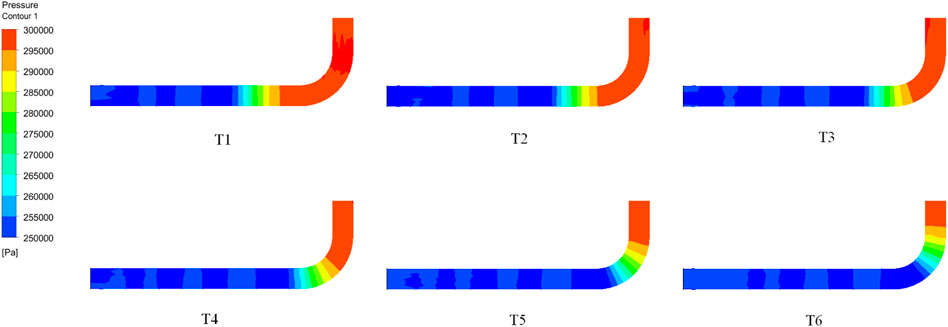
FIGURE 7. Pressure contour of the corresponding position of the negative pressure wave’s front edge in different time steps when passing through the first elbow.

Negative pressure waves are propagated in viscous fluids by causing the volumetric compression and expansion of the flow element. Viscosity includes turbulent viscosity and molecular viscosity. In turbulence, vortex viscosity is much larger than molecular viscosity. Hence, eddy viscosity has a great influence on negative pressure wave propagation. In order to explain the phenomenon that the negative pressure wave propagate velocities vary in different parts of the pipeline, we have drawn eddy viscous contours of the axial section of the pipeline, as shown in the Figure 8, where Figure 8A is the axial section of the entire pipeline, and Figure 8B is a partial enlarged view at the first elbow. As can be seen from Figure 8A, the vortex viscosity at the elbow is significantly greater than that of a straight pipe. From Figure 8B, we can see more clearly that the vortex viscosity is larger in the local range near the axis of the elbow, and decreases gradually near the wall, but it is still larger than the straight pipe.

FIGURE 8

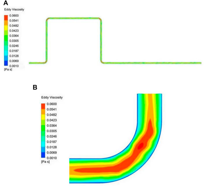
FIGURE 8. Eddy viscous contours of the axial section of the pipeline: (A) axial section of the entire pipeline, (B) partial enlarged view at the first elbow.

Figure 9 is a turbulent kinetic frequency contours of the axial section of pipeline and a partial enlarged view of its first elbow. The unit of turbulent kinetic frequency in the Figure 9 is Hz. As can be seen from Figure 9A, the distribution of the turbulent kinetic frequency contour shows obvious differences in the entire section of the pipeline, emphasizing the different turbulent kinetic frequencies at the straight pipeline section and the elbow. It can be seen from the magnitude that the turbulence kinetic frequency at the four elbows in the pipeline is generally the same, but all are slightly larger than the straight pipeline. As can be seen from Figure 9B, there is a turbulent kinetic frequency transition zone between the straight pipe and the first elbow. As the transition zone develops, the turbulent frequency starts to increase, which means that the amount of pulsation at this position when the negative pressure wave passes through the transition zone. There is a significant increase in the frequency, so the vibration frequency of the fluid element is strengthened there. Due to the structural difference between the elbow and the straight pipe, the vibration frequency of the flow element at the elbow is larger, and the frequency of viscous absorption between the flow element and the flow element becomes larger.

FIGURE 9

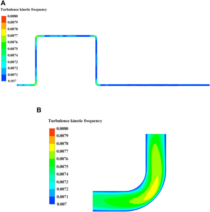
FIGURE 9. Turbulent kinetic frequency contours of the axial section of the pipeline: (A) axial section of the entire pipeline, (B) partial enlarged view at the first elbow.

Concept and formula of equivalent length of elbow based on negative pressure wave method

In order to solve the above problems and facilitate a systematic integration of the negative pressure wave propagation velocity in the elbow and the straight pipe, we propose the concept of the equivalent length of the elbow. The more common equivalent length refers to the length of the pipe corresponding to the frictional resistance of the same pipe diameter, that is, equivalent to the local resistance in the hydraulic calculation of the system. The equivalent length of the elbow here refers to the length of the corresponding straight pipe that the negative pressure wave passes through the elbow and is converted into the same pipe diameter. After a large number of numerical simulations, we found that the main parameters affecting the equivalent length of the elbow include the elbow angle, the radius of curvature, and the elbow diameter. The influence of each parameter on the transmission characteristics of negative pressure wave in the elbow is different. Based on the qualitative and quantitative analysis, and as the radius of curvature approaches infinity, equivalent length tends to original length, we proposed the formula for calculating the equivalent length of the elbow, and summarized the different propagation laws of the negative pressure wave in the elbow and the straight pipe. The formula for calculating the equivalent length of an elbow is as follows:

$L_{eq}=L\times \left[{\int }_0^{\frac{2{\rho }^{\prime }}{R}}{e}^{-t}dt+\frac{0.6R}{R_c}\right]\frac{2\theta }{\pi },(6)$

where L is the length of the central axis of the elbow, R is the radius of the pipe, and R_c is the radius of curvature of the elbow, θ is the angel of curvature.

Conclusion

A novel method based on weakly compressible is used in this work to research the propagation of negative pressure wave characteristics in a multi-elbow pipe. Some main conclusions can be obtained:

1) The novel method can be used to detect the propagation of negative pressure waves at multiple monitoring points. The propagation velocity in elbow is 1.4% higher than that in straight pipe when the length of the pipeline axis is used as the propagation distance of the negative pressure wave.

2) By simulations of pipelines with the different curvature radius, it is found that the backflow phenomenon occurs near the outside of the elbow. Therefore, the different propagation paths of the negative pressure wave at different positions, resulting in a large difference in the propagation velocity of the negative pressure wave in the elbow and the straight pipe.

3) The eddy viscosity and turbulent kinetic frequency at the elbow axis are 12.2% and 5.4% higher than those at the straight pipe. Therefore, the calculation formula of the equivalent length of the elbow is obtained and the applicability is verified, which integrating the difference of negative pressure wave propagation between the elbow and the straight pipe.

4) The simulation process using the new method can more accurately represent the specific phenomenon of negative pressure wave transmission in the elbow, and the equivalence length equation of the elbow in the negative pressure wave leakage localization method derived from the study can verify the applicability of the weakly compressible model. In addition, in practical engineering, dynamic pressure sensors placed at both ends of the required pipeline and its extension are used to capture the negative pressure wave generated due to pipe leakage, and the determination of the leakage point is done by calculating the time difference between the two ends of the pipe receiving the negative pressure wave generated by the leakage. This work can be widely used in engineering practice in long-distance transportation of oil pipelines and pipeline transportation of chemical materials, etc. The proposed elbow equivalent length formula to correct the error in the transmission speed of negative pressure waves in the elbow provides a more accurate method for leak detection and location. Therefore, the results of the simulation analysis of multi-elbow pipeline leakage based on the weakly compressible model are meaningful and fully validate the applicability of the method to the pipeline flow field.

Data availability

The raw data supporting the conclusions of this article will be made available by the authors, without undue reservation.

Author contributions

PL contributed with conceptualization and writing original draft preparation. XK and RH carried out the experimental validation. All authors have read and agreed to the published version of the manuscript.

Funding

The present work is financially supported by the Key R&D Program of Zhejiang Province (Grant No. 2020C03081), The Joint Funds of the National Natural Science Foundation of China (Grant No. U2006221), The National Natural Science Foundation of China (Grant No. 51676173). The supports are gratefully acknowledged.

Conflict of interest

The authors declare that the research was conducted in the absence of any commercial or financial relationships that could be construed as a potential conflict of interest.

Publisher’s note

All claims expressed in this article are solely those of the authors and do not necessarily represent those of their affiliated organizations, or those of the publisher, the editors and the reviewers. Any product that may be evaluated in this article, or claim that may be made by its manufacturer, is not guaranteed or endorsed by the publisher.

References

Ben-Mansour, R., Habib, M. A., Khalifa, A., Youcef-Toumi, K., and Chatzigeorgiou, D. (2012). Computational fluid dynamic simulation of small leaks in water pipelines for direct leak pressure transduction. Comput. Fluids. 57, 110–123. doi:10.1016/j.compfluid.2011.12.016

CrossRef Full Text | Google Scholar

Dou, C., Woldt, W., Dahab, M., and Bogardi, I. (1997). Transient ground-water flow simulation using a fuzzy set approach. Ground water 35 (2), 205–215. doi:10.1111/j.1745-6584.1997.tb00076.x

CrossRef Full Text | Google Scholar

Ferrante, M., and Brunone, B. (2003 2003). Pipe system diagnosis and leak detection by unsteady-state tests. 1. Harmonic analysis. Adv. Water Resour. 26 (1), 95–105. doi:10.1016/S0309-1708(02)00101-X

CrossRef Full Text | Google Scholar

Gao, Y., Brennan, M. J., Joseph, P. F., Muggleton, J. M., and Hunaidi, O. (2005). On the selection of acoustic/vibration sensors for leak detection in plastic water pipes. J. Sound Vib. 283 (3-5), 927–941. doi:10.1016/j.jsv.2004.05.004

CrossRef Full Text | Google Scholar

Huang, X., Li, Z., Li, J., Feng, H., Zhang, Y., and Chen, S. (2021). Acoustic investigation of high-sensitivity spherical leak detector for liquid-filled pipelines. Appl. Acoust. 174, 107790. doi:10.1016/j.apacoust.2020.107790

CrossRef Full Text | Google Scholar

Korteweg, D. J. (1878). Ueber die Fortpflanzungsgeschwindigkeit des Schalles in elastischen Röhren. Ann. Phys. Chem. 241 (12), 525–542. doi:10.1002/andp.18782411206

CrossRef Full Text | Google Scholar

Lee, N. Y., Hwang, I. S., and Yoo, H. (2001). New leak detection technique using ceramic humidity sensor for water reactors. Nucl. Eng. Des. 205 (1-2), 23–33. doi:10.1016/S0029-5493(00)00354-X

CrossRef Full Text | Google Scholar

Liu, G., and Qu, J. (1998). Guided circumferential waves in a circular annulus. J. Appl. Mech. 65 (2), 424–430. doi:10.1115/1.2789071

CrossRef Full Text | Google Scholar

Martins, N. M., Soares, A. K., Ramos, H. M., and Covas, D. I. (2016). CFD modeling of transient flow in pressurized pipes. Comput. Fluids 126, 129–140. doi:10.1016/j.compfluid.2015.12.002

CrossRef Full Text | Google Scholar

Mergelas, B., and Henrich, G. (2005 2005 2005). Leak locating method for precommissioned transmission pipelines: North American case studies,Leakage 12–14.

Google Scholar

Ming, T., and Zhao, J. (2012). Large-eddy simulation of thermal fatigue in a mixing tee. Int. J. Heat Fluid Flow 37, 93–108. doi:10.1016/j.ijheatfluidflow.2012.06.002

CrossRef Full Text | Google Scholar

Qi, M., Zhou, S., Ni, J., and Li, Y. (2016). Investigation on ultrasonic guided waves propagation in elbow pipe. Int. J. Press. Vessels Pip. 139-140, 250–255. doi:10.1016/j.ijpvp.2016.02.026

CrossRef Full Text | Google Scholar

Raisee Dehkordi, M. (1999). Computation of flow and heat transfer through two-and three-dimensional rib-roughened passages. Ann Arbor, MI: ProQuest Dissertations Publishing. (Order No. 10033976) (1774183364). Available at: https://www.proquest.com/dissertations-theses/computation-flow-heat-transfer-through-two-three/docview/1774183364/se-2.

Google Scholar

SaemI, S., Raisee, M., Cervantes, M. J., and Nourbakhsh, A. (2019). Computation of two-and three-dimensional water hammer flows. J. Hydraulic Res. 57 (3), 386–404. doi:10.1080/00221686.2018.1459892

CrossRef Full Text | Google Scholar

Verde, C., Visairo, N., and Gentil, S. (2007). Two leaks isolation in a pipeline by transient response. Adv. Water Resour. 30 (8), 1711–1721. doi:10.1016/j.advwatres.2007.01.001

CrossRef Full Text | Google Scholar

Wang, S. (2000). Propagation of pressure wave of gas-liquid two-phase flow in elbow. 14th national symposium on hydrodynamics. Beijing ,China.

Google Scholar

Willsky, A. S. (1976). A survey of design methods for failure detection in dynamic systems. Automatica 12 (6), 601–611. doi:10.1016/0005-1098(76)90041-8

CrossRef Full Text | Google Scholar

Zhang, Y., Chen, S., Li, J., and Jin, S. (2014). Leak detection monitoring system of long distance oil pipeline based on dynamic pressure transmitter. Measurement 49, 382–389. doi:10.1016/j.measurement.2013.12.009

CrossRef Full Text | Google Scholar

Nomenclature

Notation

a wave velocity (m, s^-1)

C_1ɛ, C2ɛ, C3ɛ empirical constant

D pipe diameter (m)

e pipe thickness (m)

E Young's modulus (N.m-2)

gi component of gravity acceleration in the i direction (m.s-2)

Gk turbulent energy generated by the laminar velocity gradient

(kg.m-1.s-3)

Gb turbulent energy generated by buoyancy (kg.m-1.s-3)

k turbulent kinetic energy (m2.s-2)

Kf bulk modulus of fluid (N.m-2)

L length of the central axis of the elbow (m)

L1 ∼ L4 Length of straight tube (m)

Leq Elbow equivalent length (m)

Mt turbulent Mach number

p pressure (Pa)

R pipe radius (m)

t time (s)

T 50 time steps of unsteady calculation (s)

T1 ∼ T6 the time that the negative pressure wave is at different positions in the pipeline(s)

u cross-sectional average velocity (m.s-1)

YM effect of compressible turbulent pulsating expansion on the total dissipation rate

ɛ turbulent energy dissipation rate

μ kinematic viscosity (m2.s-1)

μt turbulent kinematic viscosity (m2.s-1)

β thermal expansion coefficient

σk, σɛ prandtl coefficients in k-e turbulent model

ρ density (kg.m-3)

Rc elbow curvature radius(m)

θ elbow angle