Low carbon economic dispatch of power system at multiple time scales considering GRU wind power forecasting and integrated carbon capture

To achieve carbon neutrality in electricity, measures such as increasing the share of renewable energy sources such as wind power and achieving more accurate and faster wind power forecasting, and low carbon retrofitting of thermal power units are all important to achieve the goal. Firstly, the GRU prediction algorithm was used to forecast wind power, which performed well in terms of prediction accuracy and model training speed. Then, we continue to fully utilize the source-side low-carbon characteristics by installing flue gas bypass systems and liquid storage in carbon capture plants to form an integrated carbon capture plant operation, thereby reducing carbon emissions and the proportion of abandoned wind. Secondly, a three-stage low carbon economic dispatch model is established to reduce wind abandonment by combining wind power forecasts on different time scales. Finally, a case study was carried out using a modified IEEE-39 node system. The results show that the proposed three-stage integrated dispatching method can make full use of wind energy and achieve the goal of economic dispatching of the power system.

1 Introduction

Currently, renewable energy sources such as wind power are gradually replacing traditional fossil energy sources (Duan et al., 2021). Unlike other renewable energy sources, wind power generation is random and volatile, and has certain anti-peak characteristics. The large-scale grid connection of wind power increases the pressure on the system for peaking, and if necessary, some wind power needs to be abandoned to ensure system safety. The problem of wasted wind power is no longer negligible. The main causes of wind power wastage are shifted between generation and load peaks, the low accuracy of wind power forecasts, and the insufficient adjustment rate of thermal power units (Huang et al., 2021; Han et al., 2022; Zhu et al., 2022). Highly accurate wind power forecasting can be achieved through artificial intelligence algorithms. The problem of the adjusting rate of thermal power units can be solved by introducing integrated carbon capture plants. In conclusion, wind power can be absorbed through a reasonable dispatch control strategy, combined with multi-timescale wind power forecasting (Cheng et al., 2022; Tian et al., 2022; Wei et al., 2022).

At present, wind power forecasting focuses on the study of forecast errors and multi-time scale forecasting, and is used to improve the utilization-ratio of wind power by matching it with dispatch schedules on different timescales (Aslam and Albassam, 2022; Chen W et al., 2021). The accuracy of wind power forecasting improves as the time scale is shortened, and it is relevant that multi-timescale forecasting can correct deviations in long time scales. The wind power forecasts currently used in power system dispatching are mainly long-timescale for day-ahead dispatching. At the same time, there has been a lot of research on traditional and artificial intelligence algorithms to effectively deal with the volatility and randomness of wind power and improve its accuracy (Li et al., 2021; Sun et al., 2021). Traditional algorithms include statistical models such as autoregressive integrated moving average (ARIMA), which uses statistical methods to establish the relationship between historical and forecast values. However, traditional algorithms are poor at predicting volatility. Artificial intelligence algorithms include machine learning algorithms and neural network algorithms (Sun et al., 2021; Sahra et al., 2022). Machine learning algorithms such as least squares support vector machines (LSSVM) and support vector regression (SVR). Neural network algorithms such as convolutional neural network (CNN), recurrent neural network (RNN), long short-term memory (LSTM), and gated recurrent unit (GRU), of which RNN, LSTM, and GRU are recurrent neural networks, can store sequence history information and combine it with current input values, which are calculated and then continued into subsequent units (Tanveer and Zhang 2022). Recurrent neural networks are specifically used for time series, which can effectively improve prediction accuracy and reduce model training time.

Due to its time-series nature, LSTM and GRU have great advantages in processing wind power data. For power prediction of multiple wind turbines, CNN can be used to extract the spatial features of the data first, and then the temporal characteristics of the power series can be established by LSTM to achieve the power prediction of wind turbines (Chen et al., 2021a). When the historical data is few, the pre-trained model can be fine-tuned in the target domain with small data by transfer learning (TL) to make full use of the source domain data and improve the performance of the model on the target domain data. GRU is then used to extract temporal feature information from wind power and meteorological data (Chen et al., 2021b). For ultra-short-term wind power prediction, the key features of the input data can be extracted by CNN and the dynamic changes of the features proposed by CNN can be learned by bi-directional modeling using bidirectional gated recurrent unit (Bi-GRU) network (Meng et al., 2022). In this paper, the GRU is used to predict wind power as preparatory data for input into a dispatch model containing carbon capture technology to achieve integrated economic dispatch of the power system.

After the multi-timescale wind power forecasts have been made, they are fed into the dispatching model. Wind abandonment can be improved by considering regulation devices in the dispatch plan. Typical regulation devices are storage devices, high energy-carrying devices, pumped storage plants, etc. Conditioning devices are effective in improving wind power utilization-ratio, but energy storage devices have significant energy losses. High energy-carrying devices are often difficult to create links with wind farms due to the constraints of where the resource is located (Xiang et al., 2021; Zhang Z et al., 2022). Carbon capture devices, on the other hand, are converted from traditional thermal power plants and do not have geographical restrictions (Gao et al., 2021; Huang et al., 2022; Xie et al., 2022).

Today, coal is still the dominant fuel, and carbon capture and storage (CCS) is an important technology to combat global climate change by allowing the continued use of fossil fuels and significantly reducing CO2 emissions. However, there are potential risks associated with carbon storage and CCS is currently a high investment. CO2 transport and storage should therefore be given more consideration where coal-fired power plants have a large installed capacity and are densely distributed. The investment risk can be solved by using better capture solvents, better boiler systems, and more efficient turbines, which can effectively reduce costs and energy losses (Fan et al., 2018; Fan et al., 2021).

The dispatch mathematical model in this paper is divided into optimization objectives and constraints. The optimization objective includes the start-up and shut-down and coal consumption costs of thermal power units, the cost of wind abandonment penalties, the cost of carbon trading, the depreciation cost of carbon capture plants, and the cost of solvent losses in the carbon capture process. The CCS technology includes carbon capture, transport, and storage. However, in general, the cost of the carbon capture process is the largest and changes with the capture method, so this paper focuses on the cost of carbon capture (Fan et al., 2019). Constraints include power balance constraints, wind power output constraints, thermal unit output constraints, thermal unit climbing constraints, thermal unit start/stop constraints, and integrated carbon capture plant operation constraints.

The dispatch model in this paper includes an integrated carbon capture plant. Carbon capture and storage is an important technology for decarbonization (Qian et al., 2020; Liu et al., 2022; Nie et al., 2022). While thermal power is still the dominant energy source, the addition of carbon capture equipment to conventional thermal power plants can increase system operational flexibility while achieving low-carbon and effectively improving wind power utilization (Chen et al., 2021; Zhang G et al., 2022). Carbon capture plants have the advantage of regulating peak load curves, making them an ideal source of power to complement wind power. However, current research has mainly used split-flow carbon capture plants, where the CO2 absorption process is coupled with the CO2 resolution process, which does not allow for energy time-shifting, resulting in an increase in carbon capture energy consumption with increasing thermal power plant output, which is not conducive to achieving economics. The integrated carbon capture plant, however, introduces a liquid storage type on top of the split-flow type, which enables the decoupling of the CO2 absorption process from the CO2 resolution process and makes the system more flexible and economical to operate (Jin et al., 2021; Xing et al., 2021).

This paper first uses LSTM and GRU to forecast wind power in three dimensions (1h, 15min, and 5min), with GRU performing better in terms of both prediction accuracy and model training speed. A three-stage (day-ahead, intra-day, and dynamic) economic dispatch model for power systems with integrated carbon capture plants is then constructed, with wind power forecasts as inputs to the dispatch model, and each time scale corresponding to the other. The dispatching results show that the proposed three-stage integrated dispatching model can make full use of wind energy and achieve the goal of low-carbon economic dispatch. Section 2 presents the low-carbon mechanism analysis, Section 3 introduces the principles of the forecasting algorithm and the construction of the three-stage dispatch model, and Section 4 presents the case study validation and analysis.

The main contributions of this paper are as follows:

1) Combining wind power forecasting with power system dispatch, more accurate wind power forecasting accuracy will facilitate optimal system dispatch. This is reflected in the reduction of wind power waste and the economy of dispatching costs.

2) A combination of split-flow and liquid storage carbon capture technology has been constructed, which is based on the transformation of the original thermal power plant and does not have geographical restrictions. At the same time, the addition of liquid storage carbon capture enables the decoupling of CO2 absorption and extraction processes, making system operation more flexible.

3) Existing research mostly focuses on day-ahead dispatching. This paper combines day-ahead, intra-day, and dynamic stages, to form a three-stage dispatching model, which can improve the system energy structure and reduce wind abandonment and load loss.

2 operational mechanisms that take into account multi-timescale wind power projections and the low carbon characteristics of carbon capture plants

A carbon capture plant is a traditional thermal power plant with a flue gas bypass system or solution storage to achieve either split-flow carbon capture or liquid storage carbon capture, while a combination of the two forms of carbon capture results in an integrated carbon capture plant.

Carbon capture and storage (CCS) is an important way to achieve low carbon development in the power industry. It consists of three components: carbon capture, transport, and storage, of which the capture process is closely linked to the power plant. By converting a traditional thermal power plant into a carbon capture plant, a large amount of CO2 is separated from the flue gas emitted by the plant and processed through a series of processes to form a high concentration of CO2, which is eventually isolated from the atmosphere through geological storage and deep-sea storage.

CCS, as one of the key measures for CO2 reduction, is considered to be the most promising technology for development. Numerous studies have reported that CCS technology has an important contribution to make to the global goal of controlling temperature rise. In addition to this, CCS technology can not only improve the recovery of conventional energy but also facilitate the development and utilization ratio of unconventional energy and mineral resources. Considering the irreversible trend of the global low-carbon energy transition, accelerating the research and implementation of CCS technology is an inevitable choice to support global energy security, which is conducive to the rational allocation of energy, promoting the efficient use of resources, and effectively solving the bottleneck problem of regional development. At the same time, CCS technology can turn waste into treasure, promote the formation of new economic points, and inject vitality into the development of the market economy. Although CCS is an important way to reduce carbon dioxide emissions in the future, CCS projects still have problems such as large investment, high energy consumption and uncertain risks, and some of the key technologies are still being worked out and solved, making it difficult to play a large role in a short period. Overall, it is still at the stage of research and development and implementation, and there is still a gap between it and large-scale promotion, which requires continued in-depth research.

Carbon capture is divided into post-combustion, pre-combustion and oxygen-enriched combustion carbon capture. Post-combustion capture is the most mature technology and is widely used. This paper uses post-combustion carbon capture technology.

An integrated carbon capture plant can respond to system demand for active CO2 emissions, but can also transfer carbon capture consumption from peak load times to valley times, and absorb carbon capture energy during valley times. This improves dispatch decision flexibility while relieving operational pressure at peak load times. An integrated carbon capture plant can improve wind power utilization-ratio, but can also achieve a time-shift of carbon capture energy consumption, enabling low carbon economic operation of the system.

The transfer of energy consumption for carbon capture is achieved by the amount of fluid-rich and fluid-poor storage. The process is that when the system energy consumption increases at a certain time, the carbon capture will also be intensified and the carbon capture energy consumption will increase. At this point, the carbon capture rich-tank will start to store CO2 and not resolve it until the load is low. In summary, a liquid storage carbon capture plant can divert carbon capture energy from peak loads and increase net system output.

Figure 1 shows the internal schematic of an integrated carbon capture plant. Post-combustion carbon capture in thermal power plants consists of CO2 separation and CO2 compression. Firstly, the processed flue gas is fed into an absorption tower containing monoethanolamine (MEA) solvent. Under certain operating conditions the MEA absorbs the CO2 in the flue gas to form a rich liquid containing CO2, while the rest of the flue gas (mainly O2 and N2) is discharged directly into the atmosphere through the top of the tower. The rich liquid is then pumped into the regeneration tower, where the operating conditions are changed to achieve CO2 resolution and MEA solvent regeneration, with the resolved CO2 being compressed and stored, and the lean liquid from the regeneration tower being returned to the absorption tower to complete the recycling of the solution.

FIGURE 1

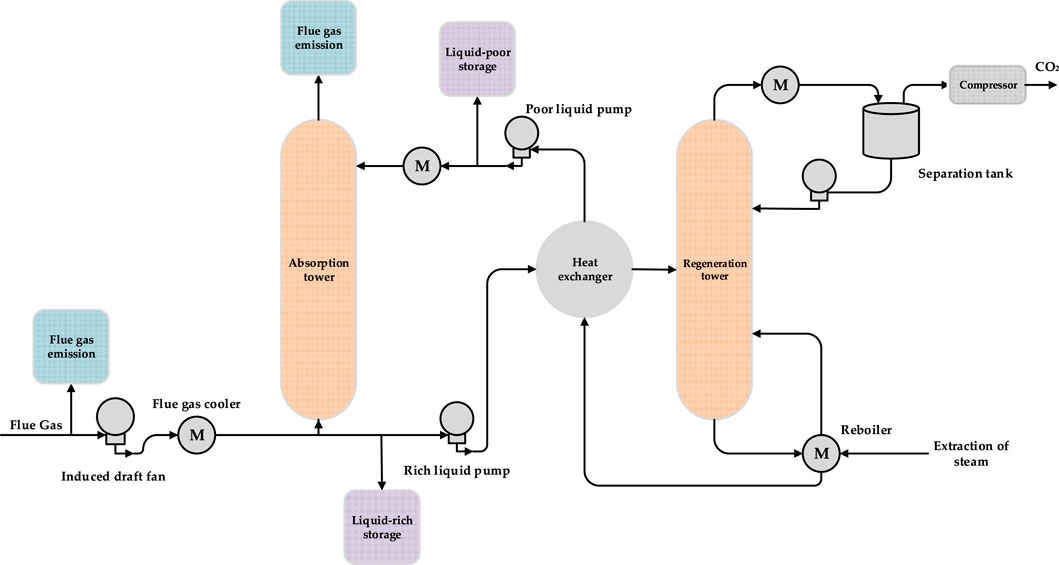
FIGURE 1. Internal schematic of an integrated carbon capture plant.

The MEA solution has a strong alkaline and is therefore often used as an absorbent for acidic gases such as CO2 and is widely used in the absorption of CO2 in coal-fired power plants. The MEA solution reacts rapidly with CO2 at 20–50°C to produce a more stable carbamate, which removes CO2 from the flue gas. The MEA solution hardly reacts with other gases in the flue gas. When the temperature of the MEA solution is raised to 105°C or higher, the carbamate can thermally decompose, thus regenerating the MEA solvent and releasing the CO2.

The reaction equation of MEA with CO2 is:

$\begin{array}{c}{\mathrm{H}}_2\mathrm{O}+{\text{MEAH}}^{+}\rightleftharpoons \text{MEA}+{\mathrm{H}}_3{\mathrm{O}}^{+}\\ 2{\mathrm{H}}_2\mathrm{O}\rightleftharpoons {\mathrm{H}}_3{\mathrm{O}}^{+}+{\text{OH}}^{-}\\ {\text{HCO}}_3^{-}+{\mathrm{H}}_2\mathrm{O}\rightleftharpoons {\mathrm{H}}_3{\mathrm{O}}^{+}+{\text{CO}}_3^{2-}\\ {\text{CO}}_2+{\text{OH}}^{-}\to {\text{HCO}}_3^{-}\\ {\text{HCO}}_3^{-}\to {\text{CO}}_2+{\text{OH}}^{-}\\ \text{MEA}+{\text{CO}}_2+{\mathrm{H}}_2\mathrm{O}\to {\text{MEACOO}}^{-}+{\mathrm{H}}_3{\mathrm{O}}^{+}\\ {\text{MEACOO}}^{-}+{\mathrm{H}}_3{\mathrm{O}}^{+}\to \text{MEA}+{\mathrm{H}}_2\mathrm{O}+{\text{CO}}_2\end{array}(1)$

The net output of a carbon capture plant needs to reduce the carbon capture energy consumption, which is divided into operational energy and fixed energy consumption. The energy used to resolve CO2 in the carbon capture process is much greater than the energy used to absorb it. Thus, the mathematical model of a carbon capture plant, considering only the energy consumption for resolution and compression, is as follows.

$\{\begin{array}{c}{E}_{\mathrm{G}i,t}=e_{\mathrm{g}i}{P}_{\mathrm{G}i,t}\\ 0\le {\delta }_i\le 1\\ E_{\text{totalCO}2i,t}=E_{\text{CG}i,t}+\beta {\delta }_i{E}_{\mathrm{G}i,t}\\ 0\le E_{\text{totalCO}2i,t}\le \eta \beta e_{\mathrm{g}i}{P}_{\mathrm{G}i,\max }\\ P_{\mathrm{B}i,t}=\lambda E_{\text{totalCO}2i,t}\\ P_{\mathrm{G}i,t}=P_{\mathrm{J}i,t}+P_{\mathrm{D}i}+P_{\mathrm{B}i,t}\end{array}(2)$

where $P_{\mathrm{G}i,t}$ is the total output of unit i at time t. $e_{\mathrm{g}i}$ is the carbon intensity of unit i. $E_{\mathrm{G}i,t}$ is the total CO2 emissions of unit i at time t. $\delta$ is the flue gas split ratio of unit i. $\beta$ is the carbon capture efficiency. $E_{\text{CG}i,t}$ is the amount of CO2 to be captured supplied by the solution storage of unit i in period t. $E_{\text{totalCO}2i,t}$ is the total CO2 captured by unit i at time t. $\eta$ is the maximum operating factor of the solution regeneration and the compression tower. $P_{\mathrm{G}i,\max }$ is the maximum output of unit i at time t. $\lambda$ is the energy consumption required to capture each unit of CO2. $P_{\mathrm{B}i,t}$ is the operational energy consumption of carbon capture plant i at time t. $P_{\mathrm{D}i}$ is the fixed energy consumption of carbon capture plant i. $P_{\mathrm{J}i,t}$ is the net output of carbon capture plant i at time t.

From eq. (2), it can be deduced that the net output range for integrated carbon capture plants and the split-flow carbon capture plants are:

$\begin{array}{l}{P}_{\mathrm{G}i,\min }-\lambda \eta \beta {\delta }_{i\max }{e}_{\mathrm{g}i}{P}_{\mathrm{G}i,\max }-P_{\mathrm{D}i}\le P_{\mathrm{J}i,t}\le P_{\mathrm{G}i,\max }-P_{\mathrm{D}i}\\ P_{\mathrm{G}i,\min }-\lambda \beta {\delta }_{i\max }{e}_{\mathrm{g}i}{P}_{\mathrm{G}i,\min }-P_{\mathrm{D}i}\le P_{\mathrm{J}i,t}\le P_{\mathrm{G}i,\max }-P_{\mathrm{D}i}\end{array}(3)$

It can be seen from the equations that the integrated carbon capture plants have a greater net output range than the split flow plants, using Figure 2 depicts the net output range of the three plants.

FIGURE 2

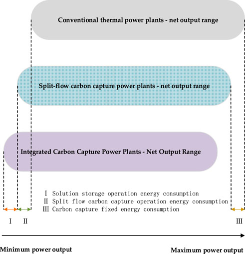
FIGURE 2. Net output range for conventional thermal power plants, split-flow carbon capture plants and integrated carbon capture plants.

Compared to conventional thermal power plants, split-flow carbon capture plants have a lower net bottom output limit. The time-shifting nature of the carbon capture energy consumption of a carbon capture plant, based on the addition of a storage tank to the plant, results in a lower net bottom output limit for an integrated carbon capture plant. With the same rotating reserve requirements, the lower net output limit facilitates the absorption of wind power, resulting in energy savings and emission reductions. In addition, carbon capture plants can change the plant operation by changing the flue gas split ratio, whereas traditional thermal plants require boiler adjustments. Changing the flue gas split ratio is more time-sensitive and can effectively address wind abandonment and load loss.

Wind power is a key source for decarbonizing power system because it is low-cost and zero-carbon. However, unlike other forms of energy, wind power generation is random and highly volatile, and exhibits certain anti-peak characteristics. Nowadays, the large-scale grid connection of wind power puts greater pressure on system peaking, and sometimes some of the wind energy has to be abandoned to ensure system safety. Shortening the forecast scale can effectively improve the accuracy of wind power forecast, while the lack of efficiency of thermal regulation can be solved by fast regulation devices (carbon capture plants). If the two are combined, more wind energy can be absorbed. At the same time, low wind power forecasting accuracy requires flexibility in the dispatch. Therefore, improving the accuracy of wind power forecasting, promoting the absorption of wind power and reducing the level of system carbon emissions remain topical issues.

There are two ways to improve the accuracy of wind power forecasting, one is to shorten the time scale and the other is to use forecasting algorithms that conform to the pattern of wind power generation.

The accuracy of wind power forecasting improves with the shortening of the time scale. The results of wind power forecasting on different time scales are sent to the dispatching model, which helps to correct the deviation between the long-time scale pre-dispatching plan and the short time scale working conditions. At present, the economic dispatch of power systems containing wind power is mostly concentrated in the long-time scale dispatch phase, so it is of practical significance to study the combination of wind power prediction and dispatch on multiple time scales.

Because of the stochastic and highly volatile nature of wind power, the use of forecasting algorithms that match its characteristics has a crucial impact on the results. Traditional statistical model-based forecasting algorithms establish a mapping relationship between input and output quantities and do not focus on the influence of the stochastic component, nor do they take into account the decaying nature of the stochastic component over time. In the paper, GRU is used to forecast wind power. As a variant of the RNN, GRU is suitable for processing time series data and can effectively extract the correlation information between each time sub-series. Compared with the LSTM, GRU has fewer parameters and is more computationally efficient.

Due to the large-scale wind power grid connection, the traditional day-ahead dispatching strategy is no longer sufficient to meet the requirements of system safety and economy. Combining multi-time-scale wind power forecasting with multi-time-scale dispatching enables the system to have a deeper regulation range and a faster regulation rate, based on the energy transfer characteristics of carbon capture plants. The deeper regulation range allows for the absorption of wind abandonment during the day-ahead and intra-day dispatch stages. The faster regulation rate allows the system to participate in the dynamic dispatch stage.

The three-stage dispatching strategy is: the day-ahead stage sets the next day’s 24 h unit start-up and shutdown and output plan, the intra-day stage can correct the unit output according to the 15min short-term wind power forecast, and the dynamic stage can adjust the net output of the carbon capture plant according to the 5-min ultra-short-term wind power forecast.

The carbon capture plant can increase or decrease the energy consumption of the carbon capture equipment at any time in response to system requirements, changing the net output and increasing the speed of output regulation of the thermal plant. At the same time, due to the presence of carbon capture consumption, the net output of the carbon capture plant is lower and the regulation range is deeper. The specific mechanisms for eliminating wind abandonment are as follows.

For the same standby requirements, carbon capture plants have a lower net output threshold, thus enabling less wind to be abandoned. On the one hand, carbon capture plants can provide more up-rotating reserves. When more up-rotation reserve is required, conventional thermal plants can only turn on additional units, resulting in wind abandonment. Carbon capture plants, do not need to restart units with the required up-rotation reserve, which effectively reduces wind abandonment.

On the other hand, carbon capture equipment can change the net output of a carbon capture plant by adjusting the shunt ratio, essentially regulating the rate of steam extraction, which is faster. Compared to conventional thermal power plants, which require 5–10 min for standby response, carbon capture plants can respond to standby requirements in less than 5 min. As a result, conventional thermal plants are unable to respond quickly to a 5-min wind forecast during the dynamic stage, whereas carbon capture plants have limited regulation but can effectively reduce wind abandonment.

3 Multi-timescale low carbon economic dispatch model

3.1 Predictive model

3.1.1 Pre-processing

Exponential weighted moving average (EWMA) is often used to describe trends of time series. It considers the high weight of recent data, at the same time, gradually reduces the weight of recent data to compensate overall trend. This feature can describe future trends in wind power and further enrich the dataset.

The process of constructing the EWMA feature is as follows. For wind power, $n$ is the total number of time points.

$\{\begin{array}{c}{e}_i=l_0,i=\mathrm{0,1}\\ e_i=\left(1-\alpha \right)e_{i-1}+\alpha l_{i-1},i=\mathrm{2,3}\dots n\\ e_i=\left(1-\alpha \right)e_n+\alpha l_n,i>n\end{array}(4)$

Where, $\alpha$ is the smoothing parameter. The value range of $\alpha$ is $(\mathrm{0,1}]$, and differential evolution method is used to minimize the objective function to obtain the optimal $\alpha$ value. The calculated objective is as follows.

$\alpha =\mathrm{a}\mathrm{r}\mathrm{g}\mathrm{m}\mathrm{i}\mathrm{n}\left({\displaystyle \sum }_{i=1}^N\sqrt{{\left(l_i-e_i\right)}^2}\right)(5)$

Simple moving average (SMA) is an unweighted arithmetic average of the n values preceding a given variable. For example, a 96-point simple moving average of a 15-min wind power forecast refers to the average of the previous day’s wind power. If the power at each point is $p_1$ to $p_n$, and when calculating successive values, a new point is added while an old point is dropped out, the SMA is calculated as.

$SM{A}_{t1,n}=SM{A}_{t0,n}-\frac{p_1}{n}+\frac{p_{n+1}}{n}(6)$

Figure 3 shows the wind power (15 min) and its EWMA and SMA features for Belgium in July 2021. The red line in the figure is the EWMA, which reflects the trend of wind power in the short term and provides reference information for wind power forecasting. The blue line in the figure is the SMA. SMA is the wind power average over the first N points and is a simple extraction of the wind power trend. EWMA can extract the trend while eliminating the effect of complex noise and enriching the dataset.

FIGURE 3

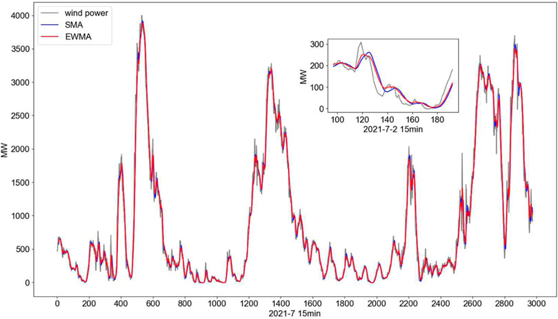
FIGURE 3. EWMA and SMA features of wind power from Belgium July 2021.

Curve features include average, minimum, maximum, and average difference values, respectively used to describe average trend and extreme value of time series data and changes of time series data on different days. For time-series data of impact quantity $V$, $V_w^i$ means impact quantity within time-window w, point $i$ changes from 1 to 4. Equations show calculation of $V_{\text{mean}}$ and $V_{{\text{mean}}_{-}\text{diff}}$. The time-window $w$ is set as four for insight into hourly changes in wind power.

$V_{\text{mean}}={\displaystyle \sum }_{i=1}^w{v}_w^i/w(7)$

$V_{{\text{mean}}_{-}\text{diff}}={\displaystyle \sum }_{i=2}^w\left(v_w^i-v_w^{i-1}\right)/\left(w-1\right)(8)$

Figure 4 shows the curve characteristics of wind power. Constructing curve features for wind power can maximize the use of data trends and help the model learn. Using average, extreme and average difference values, wind power prediction models will be more sensitive. Data that is only one-dimensional is extended to four dimensions. As the amount of data increases, the model can also get better prediction results.

FIGURE 4

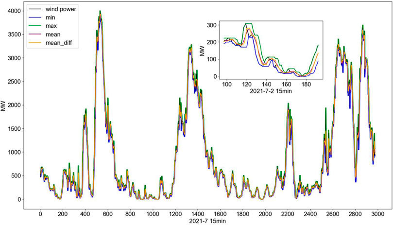
FIGURE 4. Curve features for wind power from Belgium in July 2021.

3.1.2 LSTM

Long short-term memory network (LSTM) solves the gradient disappearance of recurrent neural network (RNN) during remote transmission. LSTM currently has an excellent performance in natural language processing and time series prediction. The basic unit structure diagram is shown in Figure 5 (Farah, Aneela and Muhammad., 2021).

FIGURE 5

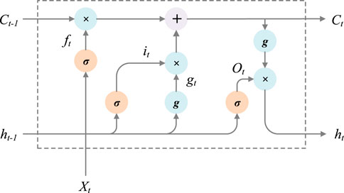
FIGURE 5. Schematic diagram of the basic unit structure of LSTM.

In Figure 5, X_t and h_t are the input and output of the basic unit at time t, i_t and f_t are the output of the input gate and forget gate at time t respectively, and O_t is the output of the outputting-gate at time t, and g_t is the unit state at time t. The specific calculation equations are as follows:

1) Input status

$g_t=\tanh \left(W_{ig}{x}_t+b_{ig}+W_{hc}{h}_{t-1}+b_{hg}\right)(9)$

2) Gating status

$i_t=sigmoid\left(W_{ij}{x}_t+b_{ii}+W_{hi}{h}_{t-1}+b_{hi}\right)(10)$

$f_t=sigmoid\left(W_{if}{x}_t+b_{if}+W_{hf}{h}_{t-1}+b_{hf}\right)(11)$

$O_t=sigmoid\left(W_{io}{x}_t+b_{io}+W_{ho}{h}_{t-1}+b_{ho}\right)(12)$

3) Memory status

$C_t=f_t\times C_{t-1}+i_t\times g_t(13)$

4) Output status

$h_t=o_t\times \tanh \left(C_t\right)(14)$

where: tanh is the hyperbolic tangent function; W is the weight vector; b is the bias.

It can be seen from Eqs (10)–(12) that LSTM fully considers the correlation between various data while making predictions, and gives sufficient space for important information. Therefore, it can usually obtain more desirable results when performing time-series data prediction.

3.1.3 GRU

Traditional convolutional networks do not have the computational ability to take into account time propagation, and the current moment output value of a recurrent neural network (RNN) is influenced by the input values of previous moments. For the wind power prediction problem, there is a time-dependent characteristic, that is, there is some correlation in the time dimension of wind power. RNN has an advantage over linear prediction models in dealing with non-linear relationships between variables. At the same time, although RNN solves the problem of long-term dependence of the prediction target, there is the problem of gradient disappearance or explosion when the network is back-propagated for calculation. The long short-term memory (LSTM) network only updates the internal states of the cells through linear transformations, allowing the information to be smoothly propagated backward across the entire time axis, thus increasing the information propagation distance, but the complex network structure of the LSTM often takes more time to train. The gated recurrent unit (GRU) simplifies the LSTM cell, which not only retains the strong time-series dependent capture capability but also effectively reduces the model training time (Niu et al., 2020).

To fully exploit the temporal characteristics of wind power to improve prediction accuracy, this section introduces a deep learning algorithm, Gated Recurrent Unit (GRU), with temporal memory capability. The deep learning framework used is TensorFlow and Keras, based on which the prediction model and structural parameters of GRU are designed to forecast on three time-scales to match the economic dispatch on each time scale for wind power.

3.1.3.1 Principle of prediction algorithm

GRU is a variant of the LSTM that simplifies the gating structure of the LSTM, thus effectively reducing the training time of the network. While the LSTM consists of three gating mechanisms, GRU unifies the forgetting and updating gates of the LSTM into a new updating gate, and thus contains only two gating mechanisms. The update gate allows adaptive control of the information flowing through the hidden unit, combining it with new inflow content for information update. The reset gate allows the contents of the memory cell to be reset. The GRU schematic is shown in Figure 6.

FIGURE 6

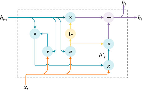
FIGURE 6. Schematic diagram of the basic unit structure of GRU.

Where $x_t$ and $h_t$ are unit input and output variables. $h_{t-1}$ and $h_t$ are internal state variables at two moments before and after the hidden layer. $g$ is a non-linear operator. In the schematic diagram +, -, 1- are linear operators. The GRU concrete state update equation is as follows.

Resetting gate

$r_t=\sigma \left(W_r{x}_t+R_r{h}_{t-1}+b_r\right)(15)$

Candidate Status:

$h_t^{\prime }=g\left(W_z{x}_t+R_z\left(r_t\odot h_{t-1}\right)+b_z\right)(16)$

Update Gate:

$u_t=\sigma \left(W_u{x}_t+R_u{h}_{t-1}+b_u\right)(17)$

New Status:

$h_t=u_t\odot h_t^{\prime }+\left(1-u_t\right)\odot h_{t-1}(18)$

where $x_t$ is the input vector at moment t. $W_r$, $W_z$ and $W_u$ are the weight matrices associated with the input status. $R_r$, $R_z$ and $R_u$ are the weight matrices associated with the recurrent state. $b_r$, $b_z$ and $b_u$ are the bias vectors. $\sigma$ is the activation function: Sigmoid. $g$ is the activation function tanh. $\odot$ is the dot product. $r_t$, $u_t$ take values in the range [0,1], if both take 1, the GRU is equivalent to an RNN. the smaller the value of $u_t$, the smaller the update of the state information of the GRU, more for the previously saved information.

The incremental cross-validation model is shown in Figure 7. Cross-validation is commonly used in the process of building predictive models and selecting model parameters. Specifically, the dataset is sliced in different ways and then various combinations of training and validation sets are fed into the model, where the training set is used for model training and the validation set is used to verify the model. With different slicing methods, data that was last used as the training set may become samples in the test set in the next iteration, thus enabling cross-validation. For time series data, incremental window cross-validation or fixed window cross-validation can be used to ensure time integrity and also to prevent future data leakage. Grid search is an automated method of adjusting parameters by continuously searching through a given range of parameter to find the best parameters. This method is even more advantageous when applied to small dataset and the sklearn provides a function GridSearchCV specifically. Applying cross validation to small dataset maximizes sample information. Also, by using models with different parameters, overfitting can be reduced to a certain extent, thus improving the robustness of the model. After grid adjustment of the parameters, the prediction accuracy and time lapse of the model are optimized.

FIGURE 7

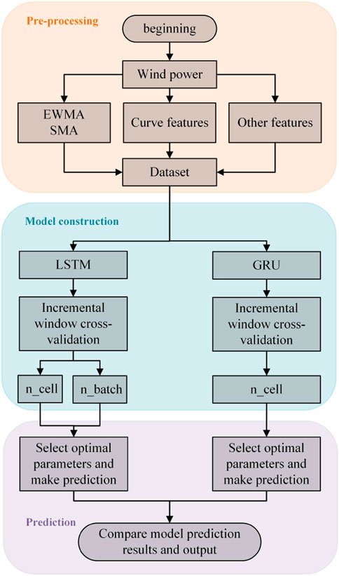
FIGURE 7. Flow chart of the prediction algorithm.

A comparison of the predictions before and after cross-validation using incremental cross-validation is shown in Figure 8, which includes the wind power prediction targets (measured and upscaled) and the GRU predictions before and after cross-validation. As can be seen from the graph, the GRU forecasts are superior in terms of prediction accuracy and time delay when using incremental cross-validation.

FIGURE 8

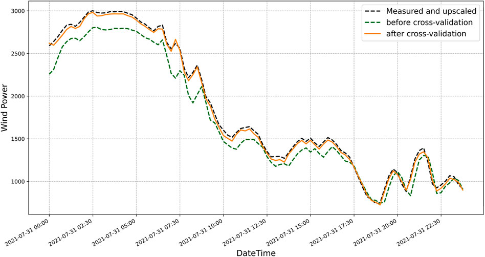
FIGURE 8. GRU predicted wind power before and after incremental cross-validation.

3.2 Low-carbon dispatch modeling considering multi-time-scale wind power forecasting and integrated carbon capture power plants

3.2.1 Multi-timescale low carbon dispatch framework

Multi-timescale wind power forecasting combined with integrated carbon capture plants can exploit the low carbon potential of the system. Firstly, the time-shifted nature of integrated carbon capture energy can both reduce the system’s lower net output limit and respond positively to the system’s need to emit CO2. Secondly, multi-timescale wind power predictions reduce wind power prediction errors and enable more accurate system dispatch plans to be made. This enables the full utilization of wind power, reduces the output of high carbon units and optimizes the low carbon and economic performance of the system. Thirdly, liquid storage carbon capture plants have a certain effect in the dynamic dispatch stage. Errors are reduced through highly accurate wind power predictions. The flue gas diversion ratio is then set in both the day-ahead and within-day phases, thus improving system dispatch flexibility, maximizing carbon capture and exploring low-carbon potential. In summary, multi-timescale wind power load predictions together with integrated carbon capture plants work together in the three stages of dispatch to optimize the system energy structure, resource allocation, reduce wind abandonment and load loss situations, and thus achieve low carbon economic dispatch.

Figure 9 shows the multi-timescale low carbon economic dispatch framework. The dispatch plan is developed 24 h in advance and the time unit is 1 h. The dispatch quantities to be determined are the unit start/stop plan and the unit output plan, which are brought into the within-day dispatch model as the determined quantities. The within-day scheduling plan is a 4 h plan with a 15min interval. Within-day scheduling is a good way of correcting the deviations between the day-ahead scheduling plan and the actual working conditions during the day. What needs to be determined in the intra-day stage is the unit output plan for the next 4 h and the results are brought into the dynamic dispatch model. The dynamic dispatch plan is advanced every 5 min to develop a post 15 min plan, to combine a highly accurate wind power forecast with the dispatch plan to adjust the carbon capture energy consumption. The amount of carbon capture energy needs to be determined during the dynamic stage.

FIGURE 9

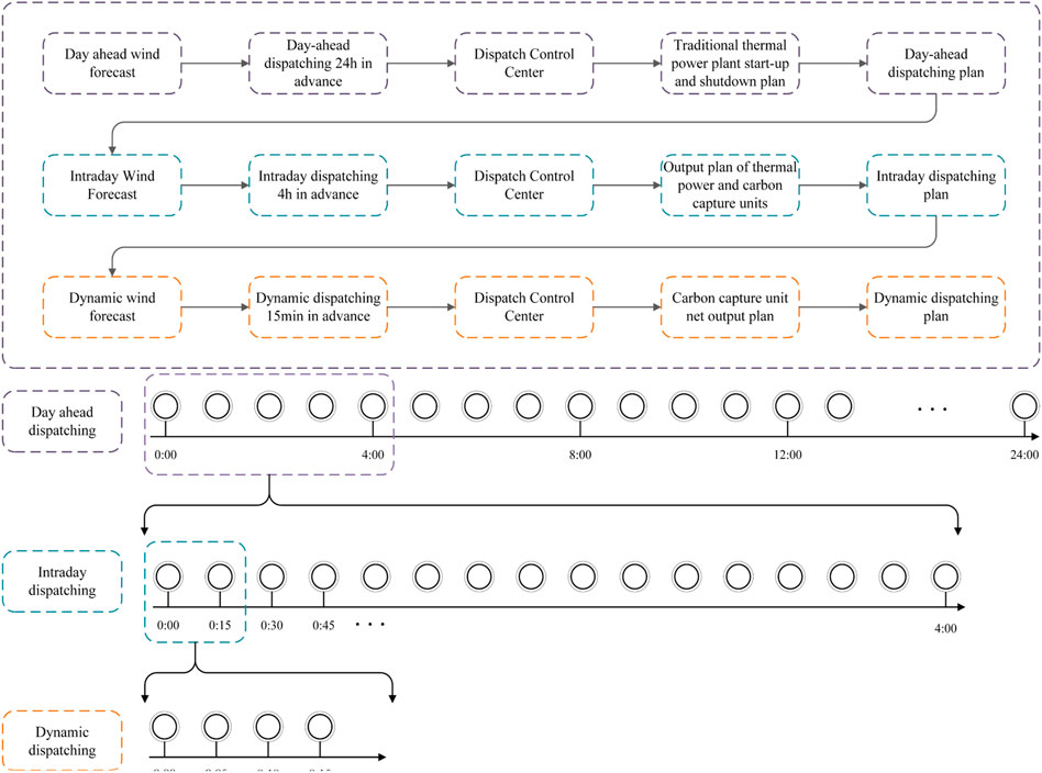
FIGURE 9. Low carbon economic dispatch framework for systems considering multi-time scale wind power predictions.

Wind power forecasting on multiple time scales can improve the accuracy and combine it with the dispatching of carbon capture plants to develop more accurate dispatching plans to effectively deal with load loss and wind abandonment while maximizing the low carbon performance of the system and reducing system costs.

3.2.2 Day-ahead dispatching model

3.2.2.1 Optimization objective

The objective function for the day-ahead dispatch stage is:

$C_1=\min \left(C_K+C_H+C_Q+C_T+C_Z+C_R\right)(19)$

1) $C_K$ is the start-up and shutdown cost of the thermal unit, $C_H$ is the coal consumption cost of the thermal unit, $C_Q$ is the penalty cost of wind abandonment, $C_T$ is the cost of carbon trading, $C_Z$ is the depreciation cost of the carbon capture plant, and $C_R$ is the cost of solvent loss in the carbon capture process.

$C_K={\displaystyle \sum }_{t=1}^{24}{\displaystyle \sum }_{i=1}^N\left(U_{i,t}\left(1-U_{i,t-1}\right)+U_{i,t-1}\left(1-U_{i,t}\right)\right)C_i(20)$

where N is the number of thermal power units. $U_{i,t}$ is the start-stop state of unit i at time t. $C_i$ is the start-stop cost of unit i.

2) Coal consumption costs for thermal power units.

$C_H={\displaystyle \sum }_{t=1}^{24}{\displaystyle \sum }_{i=1}^N{U}_{i,t}\left(a_i{P}_{\mathrm{G}i,t}^2+b_i{P}_{\mathrm{G}i,t}+c_i\right)(21)$

Where $a_i$, $b_i$ and $c_i$ is the coal consumption cost factors for unit i. $P_{\mathrm{G}i,t}$ is the total unit output of unit i at time t.

3) Cost of wind abandonment.

$C_Q={\displaystyle \sum }_{t=1}^{24}{K}_{\mathrm{q}}\left(P_{\mathrm{w},t}^{pre,1}-P_{\mathrm{w},t}\right)(22)$

$K_{\mathrm{q}}$ is the wind abandonment cost factor. $P_{\mathrm{w},t}$ is the wind power online in period t. $P_{\mathrm{w},t}^{pre,1}$ is the predicted day-ahead wind power in period t.

4) Cost of carbon capture.

$C_{\mathrm{T}}=K_{\mathrm{T}}\left(E_{\mathrm{c}}-{\displaystyle \sum }_{i=1}^N{\displaystyle \sum }_{t=1}^{24}\left({\delta }_{\mathrm{h}}{P}_{\mathrm{G}i,t}\right)\right)(23)$

$K_{\mathrm{T}}$ is the carbon trading price. $E_{\mathrm{c}}$ is the total amount of CO2 produced by thermal power units. ${\delta }_{\mathrm{h}}$ is the carbon emission allowance factor.

5) Depreciation costs of carbon capture equipment.

$C_{\mathrm{z}}=\frac{C_{\text{FL}}{\left(1+r\right)}^{N_{\text{ZJ}}}r}{365\left({\left(1+r\right)}^{N_{\text{ZJ}}}-1\right)}+\frac{P_{\text{RY}}{V}_{\text{RY}}{\left(1+r\right)}^{N_{\text{RY}}}r}{365\left({\left(1+r\right)}^{N_{\text{RY}}}-1\right)}(24)$

$C_{\text{FL}}$ is the total cost of the carbon capture equipment. $N_{ZJ}$ is the depreciable year of the carbon capture equipment. $r$ is the discount rate for the carbon capture plant project. $P_{\text{RY}}$ is the cost per unit volume of solution storage. $V_{\text{RY}}$ is the volume of solution storage. $N_{RJ}$ is the depreciable year of the solution storage.

6) The cost of solvent loss during carbon capture.

$C_{\mathrm{R}}={\displaystyle \sum }_{t=1}^{24}{\displaystyle \sum }_{i=1}^N{K}_{\mathrm{R}}\phi E_{totalCO2i,t}(25)$

$K_{\mathrm{R}}$ is the ethanolamine solution cost factor. $\phi$ is the solvent loss factor. $E_{totalCO2i,t}$ is the mass of CO2 captured by unit i at time t.

3.2.2.2 Constraints

1) Power balance constraint.

$P_{1.t}=P_{w,t}+{\displaystyle \sum }_{i=1}^N{P}_{Ji,t}(26)$

Where $P_{1.t}$ is the load. $P_{Ji,t}$ is the net output of unit i in period t. $P_{w,t}$ is the online wind power at period t.

2) Wind power output constraints.

$0\le P_{\mathrm{w},t}\le P_{\mathrm{w},t}^{pre,1}(27)$

3) Thermal power unit output constraints.

$\{\begin{array}{cc}{P}_{\mathrm{G}i,\min }\le P_{\mathrm{G}i,t}\le P_{\mathrm{G}i,\max }& U_{i,t}=1\\ P_{\mathrm{G}i,t}=0& U_{i,t}=0\end{array}(28)$

$P_{\mathrm{G}i,\min }$ is the minimum technical output of unit i. $P_{\mathrm{G}i,\max }$ is the maximum output of unit i.

4) Thermal power unit climbing constraints.

$\{\begin{array}{c}{P}_{Gi,t}-P_{Gi,t-1}\le U_{i,t}{R}_i^{\mathrm{u}}\\ P_{Gi,t-1}-P_{Gi,t}\le U_{i,t-1}{R}_i^{\mathrm{d}}\end{array}(29)$

$R_i^{\mathrm{u}}$ is the uphill climb rate of unit i and $R_i^{\mathrm{d}}$ is the downhill climb rate of thermal unit i.

5) Start/stop constraints for thermal power units.

$\{\begin{array}{c}\left(T_{i,t-1}^{\text{on}}-T_{i,\min }^{\text{on}}\right)\left(U_{i,t-1}-U_{i,t}\right)\ge 0\\ \left(T_{i,t-1}^{\text{off}}-T_{i,\min }^{\text{off}}\right)\left(U_{i,t}-U_{i,t-1}\right)\ge 0\end{array}(30)$

where, $T_{i,\min }^{\text{on}}$ is the minimum start-up time of unit i. $T_{i,\min }^{\text{off}}$ is the minimum shutdown time of unit i. $T_{i,t-1}^{\text{on}}$ is the time that unit i has been on continuously up to period t. $T_{i,t-1}^{\text{off}}$ is the time that unit i has been continuously shut down to period t. The start/stop constraint for thermal power units is intended to govern. The start/stop time must not be less than a fixed value to avoid affecting the safety of the unit.

6) Operational constraints on integrated carbon capture plants.

Carbon capture power plants add a flue gas bypass and storage tank based on a conventional thermal power plant, so their unit output constraints, creep constraints and start-stop constraints are the same as those of a conventional thermal power plant. A split-flow carbon capture plant will limit the flue gas split ratio, thus limiting the carbon capture energy consumption. Integrated carbon capture plants directly limit the amount of total CO2 resolved.

$\left(1-{\delta }_{\text{xz}}\right)\le {\delta }_i\le {\delta }_{\text{xz}}(31)$

$\{\begin{array}{l}\left(1-{\delta }_{\text{xz}}\right)\lambda \beta e_{gi}{P}_{\mathrm{G}i,t}\le P_{\mathrm{B}i,t}\\ P_{\mathrm{B}i,t}\le \eta \lambda \beta e_{gi}{P}_{\mathrm{G}i,\max }-\left(1-{\delta }_{\text{xz}}\right)\lambda \beta e_{gi}{P}_{\mathrm{G}i,t}\end{array}(32)$

where, ${\delta }_{\text{xz}}$ is the flue gas split ratio limit. $\lambda$ is the energy required to capture a unit of CO2. $\beta$ is the carbon capture efficiency. $e_{gi}$ is the carbon emission intensity. $P_{\mathrm{B}i,t}$ is the energy consumption to operate the carbon capture unit i at time t. $\eta$ is the maximum operating factor of the solution regeneration tower and the compression tower.

Reservoir carbon capture is an important component of integrated carbon capture. A storage solution is CO2 in the form of a compound in an alcoholic amine solution. The mass of CO2 captured using a solution volume equivalent transformation is as follows.

$V_{\text{CA}i,t}=\frac{E_{\text{CG}i,t}{M}_{\text{MEA}}}{M_{\text{CO}2}\theta C_{\mathrm{R}}{\rho }_{\mathrm{R}}}(33)$

Where $V_{\text{CA}i,t}$ is the volume of solution required to release CO2 from the solution reservoir installed in the carbon capture plant i at time t. $M_{\text{MEA}}$ is the molar mass of MEA. $M_{\text{CO}2}$ is the molar mass of CO2. $\theta$ is the amount of CO2 resolved in regeneration towers. $C_{\mathrm{R}}$ is the concentration of alcoholic amine solution. ${\rho }_{\mathrm{R}}$ is the density of the alcohol-amine solution.

The solution storage constraints mainly include the reservoir volume constraint and the reservoir volume variation constraint, as in the following equation.

$\{\begin{array}{c}{V}_{\text{FY}i,t}=V_{\text{FY}i,t-1}-V_{\text{CA}i,t}\\ V_{\text{PY}i,t}=V_{\text{PY}i,t-1}+V_{\text{CA}i,t}\\ 0\le V_{\text{FY}i,t}\le V_{\text{CR}i}\\ 0\le V_{\text{PY}i,t}\le V_{\text{CR}i}\\ V_{\text{FY}i,0}=V_{\text{FY}i,24}\\ V_{\text{PY}i,0}=V_{\text{PY}i,24}\end{array}(34)$

$V_{\text{FY}i,t}$ is the volume of solution in the liquid-rich storage of unit i at time t. $V_{\text{CA}i,t}$ is the volume of solution required to release CO2 from the solution storage installed at carbon capture plant i at time t. $V_{\text{PY}i,t}$ is the volume of solution in the depleted solution storage of unit i at time t. $V_{\text{CR}i}$ is the solution storage capacity of unit i. $V_{\text{FY}i,0}$ is the volume of solution in unit i’s liquid-rich tank at time 0. $V_{\text{FY}i,24}$ is the volume of solution in the rich tank of unit i at time 24. $V_{\text{PY}i,0}$ is the volume of solution in the liquid-poor tank of unit i at time 0. $V_{\text{PY}i,24}$ is the volume of solution in the poor tank of unit i at time 24.

7) Rotating standby constraints.

$\{\begin{array}{c}{\displaystyle \sum }_{i=1}^N\min \left[R_i^{\mathrm{u}},\left(U_{i,t}{P}_{\mathrm{G}Ji,\max }-P_{\mathrm{G}Ji,t}\right)\right]\ge r_{\text{sys}}^{\text{up},t}\\ {\displaystyle \sum }_{i=1}^N\min \left[R_i^{\mathrm{d}},\left(P_{\mathrm{G}Ji,t}-U_{i,t}{P}_{\text{GJ}i,\min }\right)\right]\ge r_{\text{sys}}^{\text{down},t}\end{array}(35)$

Where $r_{\text{sys}}^{\text{up},t}$ is the required upper rotating reserve for the system at time t. $r_{\text{sys}}^{\text{down},t}$ is the required lower rotation reserve of the system at time t. $P_{\mathrm{G}Ji,\max }$ is the upper net output limit of unit i. $P_{\text{GJ}i,\min }$ is the lower net output limit of unit i.

8) flow constraints.

3.2.2.3 Power balance constraint

${\displaystyle \sum }_{i\in C_{\mathrm{G},j}}{P}_{i,t}-{\displaystyle \sum }_{\left(h,j\right)\in C_{\mathrm{F},j}}{f}_{hj,t}+{\displaystyle \sum }_{\left(h,j\right)\in C_{\mathrm{E},j}}{f}_{hj,t}-D_{j,t}=0(36)$

Where, $C_{\mathrm{G},j}$ is the set of units (thermal units, wind turbines) connected to node j. $f_{hj,t}$ is the power flow of line (h, j). $C_{\mathrm{F},j}$ is the set of lines starting at node j. $C_{\mathrm{E},j}$ is the set of lines ending at node j. $D_{j,t}$ is the load demand of node j.

Line transmission capacity and node voltage constraints. Flow analysis using DC flow.

$\begin{array}{c}{f}_{hj,t}=\frac{{\theta }_{h,t}-{\theta }_{j,t}}{x_{hj}}\\ -f_{hj}^{\max }⩽f_{hj,t}⩽f_{hj}^{\max }\\ -{\theta }_j^{\max }⩽{\theta }_{j,t}⩽{\theta }_j^{\max }\\ {\theta }_{\text{ref},t}=0\end{array}(37)$

Where, ${\theta }_{h,t}$ is the phase angle of the voltage at node h. ${\theta }_{j,t}$ is the voltage phase angle at node j. $x_{hj}$ is the reactance of line (h, j). $f_{hj}^{\max }$ is the maximum value of the transmission capacity of line (h, j). ${\theta }_j^{\max }$ is the maximum voltage phase angle. ${\theta }_{\text{ref},t}$ is the voltage phase angle of the balance node.

3.2.3 Intraday dispatching model

3.2.3.1 Optimization objective

The intra-day dispatch stage, compared to the day-ahead dispatch, is the stage where the change in the predicted wind power causes a change in the cost of wind abandonment. In addition, the cost of loss of load needs to be taken into account during this stage.

$C_2=\min \left(C_{\mathrm{H}}+C_Q+C_{\mathrm{T}}+C_Z+C_{\mathrm{R}}+C_{\mathrm{S}}\right)(38)$

$C_Q={\displaystyle \sum }_{t=1}^{\Delta T}{K}_{\mathrm{q}}\left(P_{\mathrm{w},t}^{\text{pre},2}-P_{\mathrm{w},t}\right)(39)$

$C_{\mathrm{S}}={\displaystyle \sum }_{t=1}^{\Delta T}{K}_{\mathrm{S}}{P}_{\mathrm{S},t}(40)$

Where $P_{\mathrm{w},t}^{\text{pre},2}$ is the intra-day wind power forecast in 15min $C_{\mathrm{S}}$ is the cost of the lost load. $K_{\mathrm{S}}$ is the penalty cost per unit of lost load. $P_{\mathrm{S},t}$ is the lost load power of the system at time t.

3.2.3.2 Constraints

The parts of the intraday dispatch model that change are the thermal unit climbing constraint and the rotating reserve constraint. Unit start-up and shutdown are not considered in the intraday dispatch stage, and therefore unit start-up and shutdown constraints are not considered. The unit output constraints and carbon capture operation constraints are similar to those of the day-ahead dispatch model.

1) Load balance constraint.

$P_{2.t}=P_{\mathrm{w},t}+{\displaystyle \sum }_{i=1}^N{P}_{\mathrm{J}i,t}+P_{\mathrm{S},t}(41)$

Where: $P_{2.t}$ is the predicted load within the day. $P_{\mathrm{w},t}$ is the grid power of wind power at time t. $P_{Ji,t}$ is the net output of unit i in period t. $P_{\mathrm{S},t}$ is the lost load of the system in period t.

2) Thermal power unit climbing constraints.

$\{\begin{array}{c}{P}_{Gi,t}-P_{Gi,t-1}\le U_{i,t}{R}_i^{\mathrm{u}}/4+P_{\mathrm{G}i,\max }\left(1-U_{i,t-1}\right)\\ P_{Gi,t-1}-P_{Gi,t}\le U_{i,t}{R}_i^{\mathrm{d}}/4+P_{\mathrm{G}i,\max }\left(1-U_{i,t}\right)\end{array}(42)$

3) Rotating alternate restraint.

$\{\begin{array}{c}{\displaystyle \sum }_{i=1}^N\min \left[R_i^{\mathrm{u}}/4,\left(U_{i,t}{P}_{\text{GJ}i,\max }-P_{\text{GJ}i,t}\right)\right]\ge r_{\text{sys}}^{\text{up},t}\\ {\displaystyle \sum }_{i=1}^N\min \left[R_i^{\mathrm{d}}/4,\left(P_{\text{GJ}i,t}-U_{i,t}{P}_{\text{GJ}j,\min }\right)\right]\ge r_{\text{sys}}^{\text{down},t}\end{array}(43)$

3.2.4 Dynamic dispatching model

The dynamic dispatch stage focuses on adjusting wind power output and correcting carbon capture energy consumption. The wind power data is forecasted over a very short period of 5 min. The accurate forecasts help the system to adjust the net output of the carbon capture plant, thus increasing the wind power utilization and reducing the loss of load.

3.2.4.1 Optimization objective

The adjustment target for the Dynamic dispatch stage is the carbon capture energy consumption within the carbon capture plant. The dynamic dispatch stage has a short cycle time and the start-up and shutdown of the units and the total output are already determined in the day-ahead and intra-day dispatch stages. The dynamic phase adjusts the system’s CO2 emissions, wind abandonment, and load loss by adjusting the variables within the carbon capture plant.

$C_3=\min \left(C_Q+C_{\mathrm{T}}+C_Z+C_{\mathrm{R}}+C_{\mathrm{S}}\right)(44)$

$C_{\mathrm{Q}}={\displaystyle \sum }_{t=1}^{\Delta T}{K}_{\mathrm{q}}\left(P_{\mathrm{w},t}^{pre,3}-P_{\mathrm{w},t}\right)(45)$

where: $P_{\mathrm{w},t}^{pre,3}$ is the dynamic predicted wind power.

3.2.4.2 Constraints

The dynamic dispatch phase does not take into account the thermal unit output plan as it is already established in the intraday dispatch phase. The remaining constraints such as individual unit output and carbon capture plant constraints are similar to the previous two stages.

1) Load balance constraint.

$P_{3.t}=P_{\mathrm{w},t}+{\displaystyle \sum }_{i=1}^N{P}_{\mathrm{J},t}+P_{\mathrm{S},t}(46)$

Where: $P_{3.t}$ is the dynamic forecast power of the load. $P_{\mathrm{w},t}$ is the grid power of wind power at time t. $P_{Ji,t}$ is the net output of unit i in period t. $P_{\mathrm{S},t}$ is the lost load power of the system in period t.

2) Carbon capture power regulation constraint.

The dynamic stage focuses on the adjustment of the carbon capture energy consumption, which is mainly borne by the solution storage.

$\{\begin{array}{c}\Delta P_{\text{BS}i,t}=P_{\mathrm{B}i,t}\\ \Delta P_{\text{BX}i,t}=P_{\mathrm{B}i\max }-P_{\mathrm{B}i,t}\\ P_{\mathrm{B}i\max }=\lambda \eta \beta e_{\mathrm{g}i}{P}_{\mathrm{G}i,\max }\end{array}(47)$

where: $\Delta P_{\text{BS}i,t}$ is the maximum net output adjustment for carbon capture unit i at time t. $\Delta P_{\text{BX}i,t}$ is the minimum net output adjustment value for carbon capture unit i at time t. $P_{\mathrm{B}i\max }$ is the maximum operating energy consumption of the regeneration and compression towers, in other words, the carbon capture energy consumption. $\lambda$ is the energy required to capture a unit of CO2. $\eta$ is the maximum operating factor of the regenerative and compression towers of the solution. $\beta$ is the carbon capture efficiency. $e_{\mathrm{g}i}$ is the carbon emission intensity. $P_{\mathrm{G}i,\max }$ is the maximum output of unit i.

Liquid storage carbon capture enables energy time-shifting, but at the same time, the net output regulation of the carbon capture unit should be kept within the regulation range.

$-{\displaystyle \sum }_{i=1}^n\Delta P_{\text{BX}i,t}\le {\displaystyle \sum }_{i=1}^n\Delta P_{\mathrm{J}i,t}\le {\displaystyle \sum }_{i=1}^n\Delta P_{\text{BS}i,t}(48)$

where $\Delta P_{\mathrm{J}i,t}$ is the net output adjustment of carbon capture unit i at time t.

4 Case study and analysis

4.1 Case settings

The wind power in this paper uses data from the Belgian grid in July 2021. Various forecasting algorithms were first used to forecast wind power on three time-scales, with the GRU algorithm performing well in terms of training speed and accuracy. Figure 10 shows the 15min wind power forecast results, Measured and upscaled is the raw Belgian wind power data, most recent forecast is the forecast for wind power from the Belgian grid, the SVR forecast is the result of the SVR model forecast, the LSTM forecast uses the model LSTM, and the model used in this paper is GRU, which is the GRU forecast with cross-validation labeled in the figure. The wind power is scaled to match the system of 488.3 MW(Li et al., 2021).

FIGURE 10

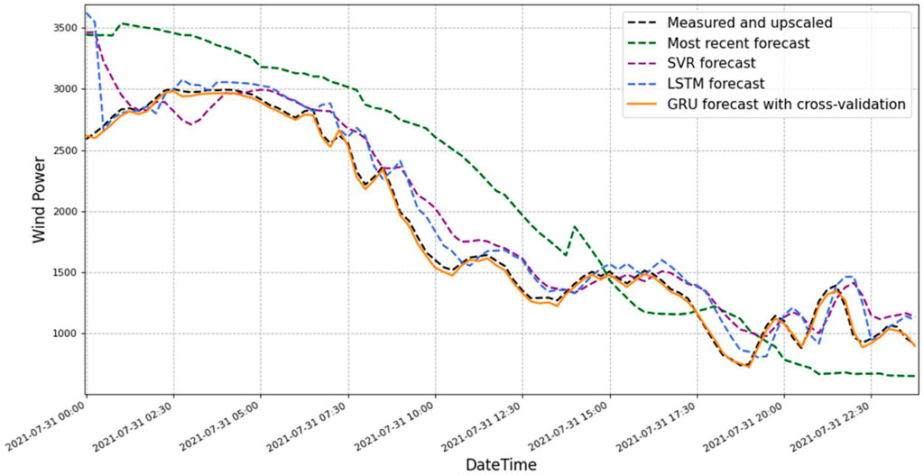
FIGURE 10. Wind power forecasting results (raw wind data\Irish grid forecasts\SVR, LSTM and GRU forecasts).

This paper is validated with a modified IEEE-39 nodal system containing 10 thermal power units. Wind farms of 198.5, 191.5, and 98.3 MW are introduced at nodes 9, 19, and 22 respectively. If the system adopts carbon capture technology, G1 and G2 are converted into carbon capture power plants, if the system does not adopt it, G1 and G2 are conventional thermal power plants. Figure 11 shows the system. Table 1 shows the relevant parameters for the thermal plant and Table 2 shows the remaining parameters to be set. The dispatch quantities are solved using the CPLEX.

FIGURE 11

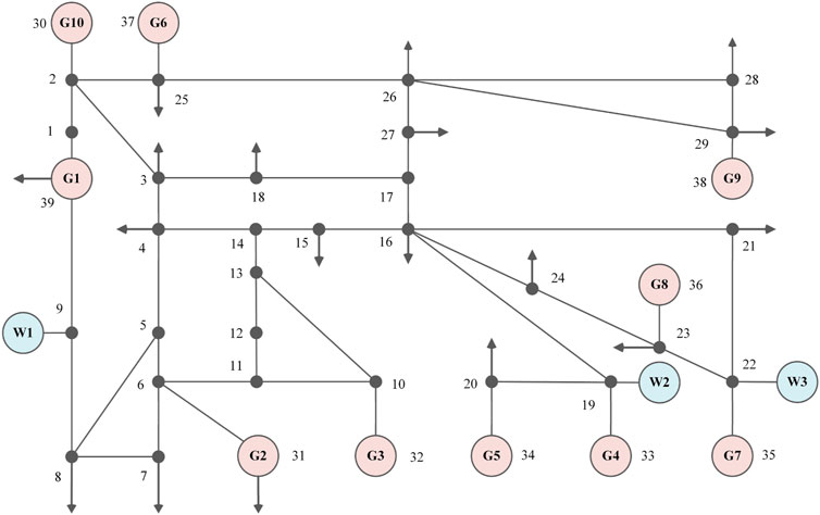
FIGURE 11. IEEE-39 node system.

TABLE 1

TABLE 1. Thermal power unit parameters (Total of 10 thermal units; input parameters include operation, cost, climbing parameters and carbon capture intensity) (Shui et al., 2019).

TABLE 2

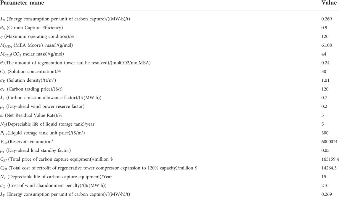
TABLE 2. Other system parameters (Mainly system size parameters and carbon capture plant operating and cost parameters) (Yu et al., 2022).

Comparison cases are set depending on whether the GRU wind power forecasts or from the Belgian grid are used.

Case 1: Consider the day-ahead dispatch of the Belgian grid with its wind power forecast (Most recent forecast) or GRU wind power forecast with carbon capture equipment.

Case 2: Consider the Belgian grid’s own wind power forecasts (Most recent forecast) or GRU wind power forecasts, with the intra-day dispatch of carbon capture equipment.

Case 3: Dynamic dispatch using the Belgian grid’s own wind power forecasts (Most recent forecast) or GRU wind power forecasts with carbon capture equipment.

4.2 Results and analysis

Figure 12 shows the results of the day-ahead dispatch with and without carbon capture devices. A shows thermal units 1 and two without carbon capture devices and B shows thermal units 1 and 2 with integrated carbon capture devices. The graphs show that after the retrofitting of carbon capture devices, there is a significant reduction in wind abandonment and a visible increase in the utilization of wind power. The analysis of the columns without carbon capture devices and the Belgian wind forecast column (with carbon capture devices) in Table 3 shows that the cost of the wind abandonment penalty is reduced by 69.032% with the installation of carbon capture devices. At the same time, the cost of carbon trading is reduced by 24.211%, and carbon emissions are reduced by 41.694% after the installation of carbon capture devices. Although the cost of running thermal power plants is higher with the addition of carbon capture devices, the total cost is reduced by 30.788%. This shows that carbon capture can reduce carbon emissions and at the same time satisfy the economy, helping to achieve low carbon economic dispatch of the power system.

FIGURE 12

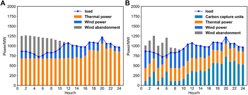
FIGURE 12. Day-ahead dispatch results with and without carbon capture devices ((A) is without carbon capture devices, (B) is with carbon capture devices).

TABLE 3

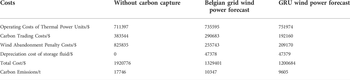
TABLE 3. Day-ahead dispatching costs.

As the load is supplied by the net thermal output and the grid power of wind power, it is only necessary to compare the net thermal output to analyze the system’s wind abandonment situation. The net output of thermal units is shown in Figure 13. As can be seen from the graph, the different times of net thermal output are concentrated between 1:00 to 12:00, and the difference in net output during the corresponding period is the difference in the amount of wind abandoned with or without carbon capture devices.

FIGURE 13

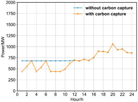
FIGURE 13. Comparison of the output of thermal power units with and without carbon capture devices.

Figure 14 shows a comparison of the dispatch results for case 1 (both with carbon capture units, using different wind power forecasts). As can be seen from the graph, when using GRU to forecast wind power, there is a certain degree of reduction in the amount of abandoned wind power due to the increased accuracy of the forecast. As can be seen from Table 3, in the day-ahead dispatching phase, the carbon transaction cost, abandonment penalty cost, total cost, and carbon emissions are reduced by 166,206$, 11,547$, 177,753$ and 1479t respectively when using GRU to forecast wind power compared to using the Belgian grid to forecast wind power, a respective decrease of 23.293%, 83.644%, 24.439%, and 12.716%. This validates the advantages of the flexible operation of carbon capture units. At the same time, by using GRU to forecast wind power, carbon capture units can capture more CO2 and effectively improve wind power utilization. Overall, the improvement in the accuracy of wind power forecasting has been proven to have a positive impact on the reduction of carbon emissions and system economics.

FIGURE 14

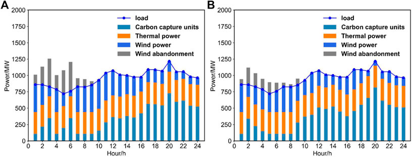
FIGURE 14. Comparison of dispatch results for case 1 ((A) considering grid forecast wind power in Belgium, (B) considering GRU forecast wind power).

In the day-ahead dispatch stage, carbon emissions depend mainly on the level of wind power consumption and the output of high-carbon units. As wind power does not emit carbon, the higher its utilization rate, the more thermal units will be replaced. At the same time, the amount of abandoned wind power decreases, the output of high-carbon thermal units decreases, and carbon emissions are reduced accordingly.

As shown in Figure 15, closely related to the net output of the thermal units is the carbon capture energy consumption. Unlike the split carbon capture unit, case 1 uses an integrated carbon capture unit, where the processes of CO2 absorption and CO2 capture are not coupled, enabling a time-shifting of the carbon capture energy consumption, so that the energy consumption is higher in the low load periods and the lower limit of the net output of the carbon capture unit is lower than that of the split type. The carbon capture units G1 and G2 are on all hours, so there is no need to increase the net output to provide down-rotation reserves, which allows more wind power to be absorbed and reduces the carbon emissions of the system compared to not installing carbon capture devices. However, due to the low load, there is still a problem of wind abandonment and the low carbon capability needs to be further explored.

FIGURE 15

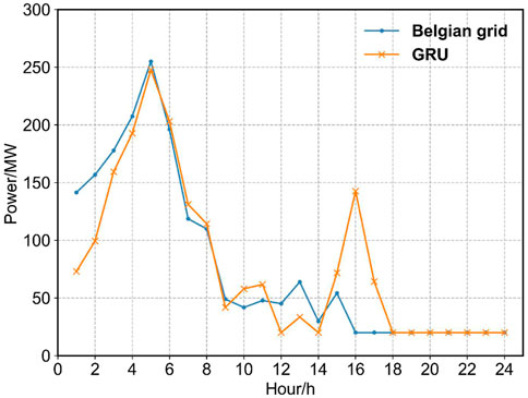
FIGURE 15. Comparison of carbon capture energy consumption using different forecast wind power in day-ahead dispatch.

Figure 16 shows a comparison of the changes in the storage tanks of case 1, where A considers the Belgian grid forecast wind power and B considers the GRU forecast wind power. As can be seen from the graph, the carbon capture units release CO2 at low load times (2:00–9:00), which shows a decrease in the amount of liquid-rich tank storage and an increase in the amount of liquid-poor tank storage. During peak load hours (16:00–24:00), CO2 is stored, showing a rise in the amount of liquid stored in the rich tank and a fall in the amount of liquid stored in the lean tank. The reduced energy consumption of the carbon capture equipment processing enables energy time-shifting, laying the foundation for low carbon economic dispatch and further reducing carbon emissions with integrated carbon capture compared to split carbon capture. Compared to the dispatch carried out by the Belgian grid predicting wind power, the use of GRU predicts that wind power has a CO2 release during the small low load hours between 13:00 and 16:00.

FIGURE 16

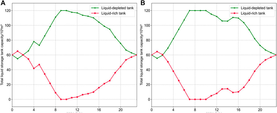
FIGURE 16. Comparison of reservoir changes in the day-ahead dispatch of Case 1 ((A) considering the Belgian grid forecast wind power, (B) considering the GRU forecast wind power).

Table 4 shows the cost table for the dispatch phase within case 2. Two scenarios are included: using the Belgian grid forecast or using the GRU forecast for wind power. Intraday dispatch does not take into account unit start-ups and shutdowns, so the costs include carbon trading costs, wind abandonment costs, lost load costs, and total costs. In the intraday scheduling phase, the total cost of using GRU wind forecasts is reduced by 177,753$ or 24.439% compared to using forecast wind. Carbon emissions are reduced by 1479t or 12.716%. The cost of the wind abandonment penalty is reduced by 11,547$, or 83.644%. It can be seen that the carbon capture system using GRU prediction wind power has the same advantages in terms of wind abandonment, cost, and carbon emissions in intra-day dispatch.

TABLE 4

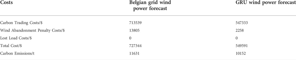
TABLE 4. Intraday dispatching costs.

The intra-day dispatch is based on the start-up and shutdown of the units determined by the day-ahead dispatch, and the intra-day dispatch output is adjusted as follows. As can be seen from Figure 17, the same wind abandonment situation exists in case 2 intra-day dispatch when using the Belgian grid forecast wind power for dispatch, with the abandonment time points mainly existing in the 0–20 period. This is because thermal power needs to reach a minimum output before it can be dispatched, and when thermal units start and stop, this can be seen as a sudden change in output power, and as the time scale shortens, due to the influence of creep. Combining all periods within a day, the remaining thermal units are adjusted less than the sudden change in thermal power caused by the start and stop of the thermal units, resulting in a wind abandonment and load loss situation. Systems containing carbon capture plants and using GRU to forecast wind power have stronger wind abandonment and load shedding characteristics.

FIGURE 17

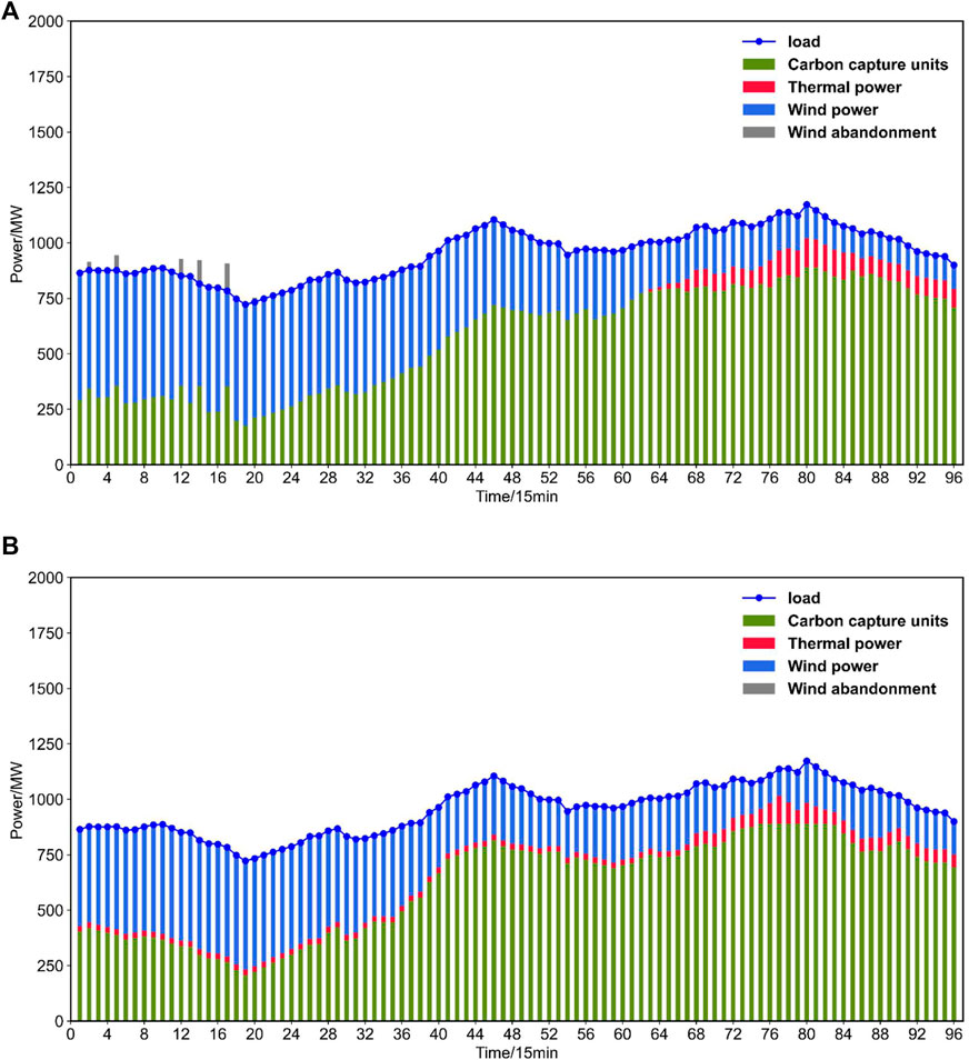
FIGURE 17. Intraday stage dispatch diagram ((A) considering Belgian grid forecast wind power, (A) considering GRU forecast wind power).

Table 5 shows the dynamic dispatch stage cost table and Figure 18 shows the case 3 dynamic dispatch diagram. Intraday dispatch provides a reference point for the total output of the thermal plant for dynamic dispatch, which regulates the carbon capture energy consumption without changing the total output.

TABLE 5

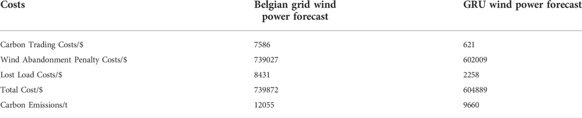
TABLE 5. Dynamic dispatching costs.

FIGURE 18

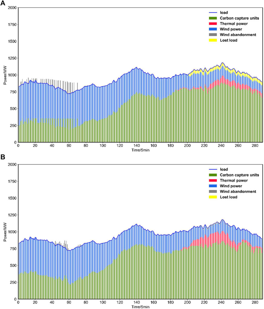
FIGURE 18. Dynamic dispatch diagram for case 3 ((A) considering Belgian forecast wind power, (A) considering GRU forecast wind power).

As can be seen from Table 5, the total cost of forecasting wind power using GRU is reduced by $134,983$ compared to the Belgian forecast of wind power in dynamic scheduling. Carbon emissions are reduced by 2395t or 19.867%. Loss of load costs is reduced by 6173$, or 73.218%. The cost of the wind abandonment penalty is reduced by 137,018$ or 18.540%. It is clear that in dynamic dispatch, the system using GRU to forecast wind power is more advantageous in terms of disposing of abandoned wind and dealing with load loss.

Figure 18 shows a graph of dynamically dispatched unit output. As can be seen from the graph, the improvement in prediction accuracy has led to greater involvement of carbon capture plants in the regulation of the 5min time scale, resulting in significant improvements in wind abandonment and load shedding, and demonstrating the effectiveness of the fast regulation characteristics of carbon capture plants. By regulating the carbon capture energy consumption to follow the changes in load and wind power, the carbon capture plant achieves the objective of absorbing the abandoned wind and reducing the lost load.

5 Conclusion

This paper constructs a multi-timescale optimal dispatch model that considers improving wind power forecasting accuracy while containing an integrated carbon capture plant and demonstrates the effectiveness of carbon capture plants in absorbing wind abandonment, coping with load loss situations, and reducing system costs, as shown in the following findings.

1) During day-ahead dispatch, the system with an integrated carbon capture plant has a 69.032% reduction in the cost of wind abandonment penalties relative to a system with only conventional plants, due to the deeper regulation range of the carbon capture plant. Carbon trading costs are reduced by 24.211% and carbon emissions are reduced by 41.694%. This demonstrates the effectiveness of carbon capture plants in improving wind power utilization and reducing carbon emissions.

2) In the intraday dispatch stage, the use of GRU to forecast wind power has led to an increase in forecast accuracy, which, when combined with carbon capture plants, can further exploit the low carbon performance of the system and improve economic efficiency. In the intra-day dispatch stage, the system’s dispatch flexibility can be improved to further reduce wind abandonment and achieve full utilization of source-side adjustable resources.

3) During dynamic dispatch, the system can respond to fluctuations in load and wind power in timely due to the fast regulation characteristics of the carbon capture plant and the improved accuracy of wind power forecasting. Its total cost is reduced by 134,983$ relative to a system that uses the Belgian grid forecast wind power. Carbon emissions were reduced by 2,395t or 19.867%. The cost of loss of load is reduced by 6173$, or 73.218%. The cost of wind abandonment penalties was reduced by 137,018$, or 18.540%. This justifies the improvement in forecasting accuracy and the use of multi-scale scheduling in dealing with wind abandonment and load loss.

Data availability statement

The original contributions presented in the study are included in the article/supplementary material, further inquiries can be directed to the corresponding author.

Author contributions

CD and YZ carried out the concepts, design, the definition of intellectual content, literature search, data acquisition, data analysis, and manuscript preparation. CD provided assistance for data acquisition, data analysis, and statistical analysis. YZ carried out literature search, data acquisition, and manuscript editing. GP and HZ performed manuscript review. All authors have read and approved the content of the manuscript and have made substantial contributions to all of the following: (1) the conception and design of the study, or acquisition of data, or analysis and interpretation of data, (2) drafting the manuscript or revising it critically for intellectual content, (3) final approval of the version to be submitted.

Conflict of interest

The authors declare that the research was conducted in the absence of any commercial or financial relationships that could be construed as a potential conflict of interest.

Publisher’s note

All claims expressed in this article are solely those of the authors and do not necessarily represent those of their affiliated organizations, or those of the publisher, the editors and the reviewers. Any product that may be evaluated in this article, or claim that may be made by its manufacturer, is not guaranteed or endorsed by the publisher.

References

Chen, W., Qi, W., Li, Y., Z, J., Zhu, F., Xie, D., et al. (2021). Ultra-short-term wind power prediction based on bidirectional gated recurrent unit and transfer learning. Front. Energy Res. 9, 808116. doi:10.3389/fenrg.2021.808116

CrossRef Full Text | Google Scholar

Chen, X., Huang, L., Zhang, X., He, S., Sheng, Z., Wang, Z., et al. (2021a). Robust optimal dispatching of wind fire energy storage system based on equilibrium optimization algorithm. Front. Energy Res. 9, 754908. doi:10.3389/fenrg.2021.754908

CrossRef Full Text | Google Scholar

Chen, X., Zhang, X., Dong, M., Huang, L., Guo, Y., and He, S. (2021b). Deep learning-based prediction of wind power for multi-turbines in a wind farm. Front. Energy Res. 9. doi:10.3389/fenrg.2021.723775

CrossRef Full Text | Google Scholar

Cheng, S., Teng, Y., Zuo, H., and Chen, Z. (2022). Power balance partition control based on topology characteristics of multi-source energy storage nodes. Front. Energy Res. 10, 843536, doi:10.3389/fenrg.2022.843536

CrossRef Full Text | Google Scholar

Duan, J., Wang, P., Ma, W., Tian, X., Fang, S., Cheng, Y., et al. (2021). Short-term wind power forecasting using the hybrid model of improved variational mode decomposition and Correntropy Long Short -term memory neural network. Energy 214, 118980. doi:10.1016/j.energy.2020.118980

CrossRef Full Text | Google Scholar

Fan, J. L., Wei, S., Shen, S., Xu, M., and Zhang, X. (2021). Geological storage potential of CO2 emissions for China’s coal-fired power plants: A city-level analysis. Int. J. Greenh. Gas Control 106, 103278. doi:10.1016/j.ijggc.2021.103278

CrossRef Full Text | Google Scholar

Fan, J. L., Wei, S., Yang, L., Wang, H., Zhong, P., and Zhang, X. (2019). Comparison of the LCOE between coal-fired power plants with CCS and main low-carbon generation technologies: Evidence from China. Energy 176, 143–155. doi:10.1016/j.energy.2019.04.003

CrossRef Full Text | Google Scholar

Fan, J. L., Xu, M., Li, F., Yang, L., and Zhang, X. (2018). Carbon capture and storage (CCS) retrofit potential of coal-fired power plants in China: The technology lock-in and cost optimization perspective. Appl. Energy 229, 326–334. doi:10.1016/j.apenergy.2018.07.117

CrossRef Full Text | Google Scholar

Farah, S., Aneela, Z., and Muhammad, M. (2021). A novel genetic LSTM model for wind power forecast. Energy 223, 120069. doi:10.1016/j.energy.2021.120069

CrossRef Full Text | Google Scholar

Gao, Q., Zhang, X., Yang, M., Chen, X., Zhou, H., and Yang, Q. (2021). Fuzzy decision-based optimal energy dispatch for integrated energy systems with energy storage. Front. Energy Res. 9, 809024. doi:10.3389/fenrg.2021.809024

CrossRef Full Text | Google Scholar

Han, H., Wei, T., Wu, C., Xu, X., Zang, H., Sun, G., et al. (2022). A low-carbon dispatch strategy for power systems considering flexible demand response and energy storage. Front. Energy Res. 10, 883602. doi:10.3389/fenrg.2022.883602

CrossRef Full Text | Google Scholar

Han, L., Jing, H., Zhang, R., and Gao, Z. (2019). Wind power forecast based on improved Long Short Term Memory network. Energy 189, 116300. doi:10.1016/j.energy.2019.116300

CrossRef Full Text | Google Scholar

Huang, X., Wang, K., Zhao, M., Huan, J., Yu, Y., Jiang, K., et al. (2022). Optimal dispatch and control strategy of integrated energy system considering multiple P2H to provide integrated demand response. Front. Energy Res. 9, 824255. doi:10.3389/fenrg.2021.824255

CrossRef Full Text | Google Scholar

Huang, Y., Li, P., Zhang, X., Mu, B., Mao, X., and Li, Z. (2021). A power dispatch optimization method to enhance the resilience of renewable energy penetrated power networks. Front. Phys. 9. doi:10.3389/fphy.2021.743670

CrossRef Full Text | Google Scholar

Jin, H., Teng, Y., Zhang, T., Wang, Z., and Deng, B. (2021). A locational marginal price-based partition optimal economic dispatch model of multi-energy systems. Front. Energy Res. 9. doi:10.3389/fenrg.2021.694983

CrossRef Full Text | Google Scholar

Li, X., Wu, X., Gui, D., Hua, Y., and Guo, P. (2021). Power system planning based on CSP-CHP system to integrate variable renewable energy. Energy 232, 121064. doi:10.1016/j.energy.2021.121064

CrossRef Full Text | Google Scholar

Liu, C., Wang, C., Yin, Y., Yang, P., and Jiang, H. (2022). Bi-level dispatch and control strategy based on model predictive control for community integrated energy system considering dynamic response performance. Appl. Energy 310, 118641. doi:10.1016/j.apenergy.2022.118641

CrossRef Full Text | Google Scholar

Meng, Y., C, C., Huo, J., Zhang, Y., Murad, M. A. N. H., Xu, J., et al. (2022). Research on ultra-short-term prediction model of wind power based on attention mechanism and CNN-BiGRU combined. Front. Energy Res. 10. doi:10.3389/fenrg.2022.920835

CrossRef Full Text | Google Scholar

Nie, Q., Zhang, L., Tong, Z., Dai, G., and Chai, J. (2022). Cost compensation method for PEVs participating in dynamic economic dispatch based on carbon trading mechanism. Energy 239, 121704. doi:10.1016/j.energy.2021.121704

CrossRef Full Text | Google Scholar

Niu, Z., Yu, Z., Tang, W., Wu, Q., and Marek, R. (2020). Wind power forecasting using attention-based gated recurrent unit network. Energy 196, 117081. doi:10.1016/j.energy.2020.117081

CrossRef Full Text | Google Scholar

Qian, T., Tang, W., and Wu, Q. (2020). A fully decentralized dual consensus method for carbon trading power dispatch with wind power. Energy 203, 117634. doi:10.1016/j.energy.2020.117634

CrossRef Full Text | Google Scholar

Sahra, K., Mehdi, E., Soodabeh, S., and Hosein, M. S. (2022). A high-accuracy hybrid method for short-term wind power forecasting. Energy 238, 122020. doi:10.1016/j.energy.2021.122020

CrossRef Full Text | Google Scholar

Shui, Y., Gao, H., Wang, L., Wei, Z., and Liu, J. (2019). A data-driven distributionally robust coordinated dispatch model for integrated power and heating systems considering wind power uncertainties. Int. J. Electr. Power & Energy Syst. 104, 255–258. doi:10.1016/j.ijepes.2018.07.008

CrossRef Full Text | Google Scholar

Sun, Z., Zhao, M., Dong, Y., Cao, X., and Sun, H. (2021). Hybrid model with secondary decomposition, random forest algorithm, clustering analysis and long short memory network principal computing for short-term wind power forecasting on multiple scales. Energy 221, 119848. doi:10.1016/j.energy.2021.119848

CrossRef Full Text | Google Scholar

Tanveer, A., and Zhang, D. (2022). A data-driven deep sequence-to-sequence long-short memory method along with a gated recurrent neural network for wind power forecasting. Energy 239, 122109. doi:10.1016/j.energy.2021.122109

CrossRef Full Text | Google Scholar

Tian, H., Zhao, H., Liu, C., and Chen, J. (2022). Iterative linearization approach for optimal scheduling of multi-regional integrated energy system. Front. Energy Res. 10. doi:10.3389/fenrg.2022.828992

CrossRef Full Text | Google Scholar

Wei, W., Hao, T., and Xu, T. (2022). Day-ahead economic dispatch of AC/DC hybrid distribution network based on cell-distributed management mode. Front. Energy Res. 10. doi:10.3389/fenrg.2022.832243

CrossRef Full Text | Google Scholar

Xiang, Y., Wu, G., Shen, X., Ma, Y., Gou, J., Xu, W., et al. (2021). Low-carbon economic dispatch of electricity-gas systems. Energy 226, 120267. doi:10.1016/j.energy.2021.120267

CrossRef Full Text | Google Scholar

Xie, H., Wang, W., Wang, W., and Tian, L. (2022). Optimal dispatching strategy of active distribution network for promoting local consumption of renewable energy. Front. Energy Res. 10. doi:10.3389/fenrg.2022.826141

CrossRef Full Text | Google Scholar

Xing, Q., Cheng, M., Liu, S., Xiang, Q., Xie, H., and Chen, T. (2021). Multi-objective optimization and dispatch of distributed energy resources for renewable power utilization considering time-of-use tariff. Front. Energy Res. 9. doi:10.3389/fenrg.2021.647199

CrossRef Full Text | Google Scholar

Yu, F., Chu, X., Sun, D., and Liu, X. (2022). Low-carbon economic dispatch strategy for renewable integrated power system incorporating carbon capture and storage technology. Energy Rep. 8, 251–258. doi:10.1016/j.egyr.2022.05.196

CrossRef Full Text | Google Scholar

Zhang, G, G., Wang, W., Chen, Z., Li, R., and Niu, Y. (2022). Modeling and optimal dispatch of a carbon-cycle integrated energy system for low-carbon and economic operation. Energy 240, 122795. doi:10.1016/j.energy.2021.122795

CrossRef Full Text | Google Scholar

Zhang, Z, Z., Du, J., Li, M., Guo, J., Xu, Z., and Li, W. (2022). Bi-level optimization dispatch of integrated-energy systems with P2G and carbon capture. Front. Energy Res. 9. doi:10.3389/fenrg.2021.784703

CrossRef Full Text | Google Scholar

Zhu, X., Wu, J., and Liu, D. (2022). Robust unit commitment for minimizing wind spillage and load shedding with optimal DPFC. Front. Energy Res. 10. doi:10.3389/fenrg.2022.877042

CrossRef Full Text | Google Scholar