An Improved Informer Model for Short-Term Load Forecasting by Considering Periodic Property of Load Profiles

Short-term load forecasting (STLF) is an important but a difficult task due to the uncertainty and complexity of electric power systems. In recent times, an attention-based model, Informer, has been proposed for efficient feature learning of lone sequences. To solve the quadratic complexity of traditional method, this model designs what is called ProbSparse self-attention mechanism. However, this mechanism may neglect daily-cycle property of load profiles, affecting its performance of STLF. To solve this problem, this study proposes an improved Informer model for STLF by considering the periodic property of load profiles. The improved model concatenates the output of Informer, the periodic load values of input sequences, and outputs forecasting results through a fully connected layer. This makes the improved model could not only inherit the superior ability of the traditional model for the feature learning of long sequences, but also extract periodic features of load profiles. The experimental results on three public data sets showed its superior performance than the traditional Informer model and others for STLF.

1 Introduction

Short-term load forecasting (SLTF) is of significant importance in the operation of electric power systems Sinha et al. (2021); Zhang et al. (2021). It provides electrical utilities the load values of the coming hours or days to enable them to draw up cost-efficient electrical plans Mashlakov et al. (2021). Take an electrical utility of 10,000 MW with the mean absolute percentage error (MAPE) approximately 4% as an example. If the MAPE was decreased by 1%, its production cost could be reduced by 0.6–1.6 million USD annually Ma (2021). However, STLF is challenged by the uncertainty of electric power systems.

Until now, researchers proposed a number of SLTF methodologies to handle this challenge. These methods can typically be classified into two categories according to what algorithms they use, namely, the statistical and machine learning methods. Both types of methods exhibit their advantages. Statistical methods are more interpretable than those using machine learning algorithms, but they usually need statistical assumptions that make capturing the underlying stochastic progress of load profiles difficult Dumas et al. (2022). Different to statistical ones, machine learning-based methods transform raw data into feature vectors through carefully designed feature extractors and proved their superior ability to address hidden nonlinearity in historical data sets compared to those using statistical algorithms Panapakidis (2016); Zahid et al. (2019); Chicco and Ilie (2009); Wang et al. (2018).

Since 2006, the deep learning (DL) technique has been developed greatly and witnesses its success in many applications. DL is a set of end-to-end machine learning methods that allows a neural network to automatically discover representations from raw data for the regression or classification task LeCun et al. (2015). Compared to conventional machine learning methods, DL-based methods show better performance for non-linear feature learning and are able to model complex non-linear systems. Therefore, in the area of STLF, many DL-based models have been proposed.

The recurrent neural network (RNN) or the long short-term memory neural network (LSTM) is among the most widely used DL models in this area Kong et al. (2018); Shi et al. (2018). The reason is that RNN or LSTM is a kind of neural network that takes sequence data as input and recurs in the direction of the sequence, and it proved to be superior for non-linear feature learning of sequence data than other types of neural network. Therefore, a number of LSTM based STLF models have been developed. For example, Bedi et al. proposed an LSTM based model that predicts the load of coming 15 min by considering season, day, and interval data Bedi and Toshniwal (2019). Next, Shi et al. proposed a new deep pooling RNN model to perform for STLF at the household level, which outperforms classical deep RNN model in terms of RMSE Shi et al. (2018). Zang et al. combined LSTM and self-attention mechanism for the day-ahead residential load forecasting Zang et al. (2021). Furthermore, some studies try to combine RNN or LSTM with a convolutional neural network (CNN) to increase the precision of load forecasting. In these models, the CNN is first used to extract local features, the results of which are then flattened and fed into the LSTM layers. For example, Sharda et al. proposed an ensemble DL model that combines CNN and LSTM for the STLF at appliance-level Sharda et al. (2021). A unified customer level STLF framework that uses CNN and bidirectional LSTM was developed and outperforms the model that only uses a single neural network Unal et al. (2021). Predict results of these models verified that the CNN layers are able to extract effective features from multiple variables and, therefore, are able to improve the load forecasting performance of RNN-based models.

However, the LSTM model proved to be not capable to keep long-term memory from a time-series perspective Zhao et al. (2020). This makes it hard to design an RNN or LSTM based forecasting model that takes long load sequences as its input and makes capturing long-range dependency from long sequences of load series data impossible, thus affecting the performance of load forecasting. In recent times, attention-based DL models, such as Transformer, showed superior performance in capturing long-term dependencies than RNN or LSTM model Vaswani et al. (2017). They utilize the self-attention mechanism to reduce the maximum length of network signals and avoid the recurrent structure. But, conversely, the time complexity and memory usage of the self-attention mechanism are O (L²), which limits its application to feature learning of long sequences. To address this, Zhou et al. proposed an efficient Transformer-based model, named Informer, in Zhou et al. (2021). It reduces the complexity of the self-attention mechanism to O (L$log$L) by designing a what is called the ProbSparse self-attention mechanism, in which only a part of the dominant queries is considered and included in the attention calculation. Since electrical load consumption data are a kind of periodic series over a long period of time, the ProbSparse self-attention mechanism of Informer may neglect periodic features of load profiles.

To solve this problem, this paper presents an improved Informer model for STLF by considering the periodic property of load profiles. First, a historical data set is normalized and divided into three subsets without overlaps, namely the training, validation, and testing sets. Then, two input matrices are constructed from each of the three subsets. After that, the input representation method of the Informer model is utilized for the input matrices to capture both global hierarchical and agnostic time stamps. Then, the results of the input representation are fed into two sets of CNN networks. To conclude, the improved Informer model completes the load forecasting. The proposed STLF model has been tested on three public data sets, and the experimental results showed more precise load forecasting than others.

The main contributions of this paper are the following: 1) the traditional Informer model is improved by considering the periodic property of load profiles; 2) by the serial connection of the Informer and CNN networks, the proposed STLF model is able to extract not only long-range dependency, but also local features from long sequences of load and meteorological data.

The rest of this paper is organized as follows. Section 2 describes the proposed STLF model. The experimental results are shown in Section 3, and a brief conclusion is given in Section 4.

2 Methods

In this section, the proposed STLF model will be described in detail. Figure 1 shows the architecture of the proposed model, which is encoder-decoder type. First, load and meteorological sequences of a data set are used to build the input matrices, X_en and X_de, for the encoder and decoder of the proposed model, which will then be represented and fed into two sets of CNN networks, respectively. After that, the Informer model receives the results of the CNN module, and its output is combined with the periodic load values of the input load sequence to form a fully connected layer, which outputs the load value of the moment to be predicted.

FIGURE 1

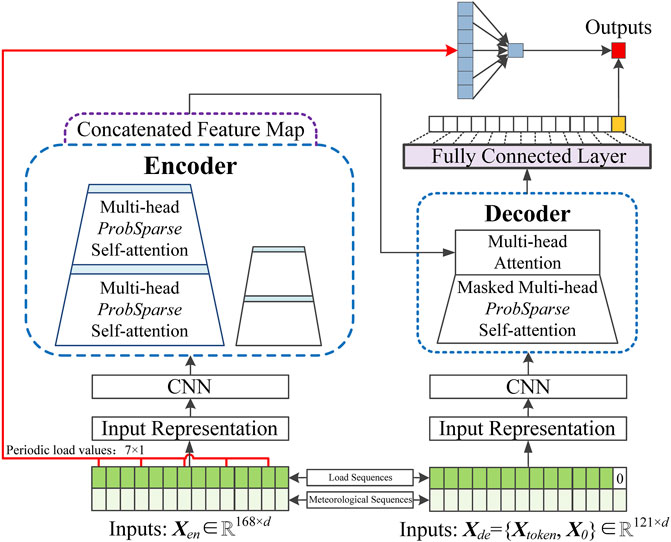
FIGURE 1. Pipeline of the proposed short-term load forecasting model.

2.1 Construction of Training, Validation, and Testing Sets

Suppose that a given historical data set $\mathit{H}\in {\mathbb{R}}^{N\times d}$ includes one load and d – 1 meteorological profiles of N days, termed as L = {l₁, l₂, … , l_N} and M = {m₁, m₂, … , m_d−1}, respectively. m_j = {m_j1, m_j2, … , m_jN} is the profile of jth meteorological data. The load and meteorological profiles of each day are first normalized by dividing their maximum values as the following:

${\mathit{l}}_i^{*}=\frac{{\mathit{l}}_i}{max\left({\mathit{l}}_i\right)},(1)$

and

${\mathit{m}}_{ji}^{*}=\frac{{\mathit{m}}_{ji}}{max\left({\mathit{m}}_{ji}\right)}.(2)$

Then, the normalized data set H^* = {L^*, M^*} is divided into three non-overlapping subsets in chronological order, termed as the training set ${\mathit{H}}_{tr}^{*}$, the validation set ${\mathit{H}}_{va}^{*}$, and the testing set ${\mathit{H}}_{te}^{*}$ respectively, which are represented as the following:

${\mathit{H}}_{tr}^{*}=\left\{{\mathit{h}}_1^{*},{\mathit{h}}_2^{*},\dots ,{\mathit{h}}_{N_{tr}}^{*}\right\},(3)$

${\mathit{H}}_{va}^{*}=\left\{{\mathit{h}}_{N_{tr}+1}^{*},{\mathit{h}}_{N_{tr}+2}^{*},\dots ,{\mathit{h}}_{N_{tr}+N_{va}}^{*}\right\},(4)$

and

${\mathit{H}}_{te}^{*}=\left\{{\mathit{h}}_{N_{tr}+N_{va}+1}^{*},{\mathit{h}}_{N_{tr}+N_{va}+2}^{*},\dots ,{\mathit{h}}_N^{*}\right\},(5)$

where N_tr and N_va are the numbers of days in the training and validation sets, respectively, and ${\mathit{h}}_i^{*}=\{{\mathit{l}}_i^{*},{\mathit{t}}_i^{*}\}$ is the i-th tensor of H^*. The testing set contains the load and temperature profiles of N − N_tr − N_va days.

2.2 Architecture of the Proposed Model

The proposed STLF model is a total encoder-decoder architecture and is made up of four separate parts: the construction of input matrices, a representation module, a CNN module, and the improved Informer model.

2.2.1 Input Matrices

For every of the three subsets, two input matrices are first constructed, termed X_en and X_de, for the encoder and decoder of the proposed STLF model, respectively. Time-series forecasting is used to predict future series at a specific time by using the series before this time. In this paper, the input of the encoder at time t includes load and temperature series before it:

$\begin{array}{cc}\hfill {\mathit{x}}_{en}^t& =\left\{{\mathit{h}}_{t-L_{en}+1}^{*},\dots ,{\mathit{h}}_{t-1}^{*},{\mathit{h}}_t^{*}\right\}\in {\mathbb{R}}^{L_{en}\times m},\hfill \\ \hfill t& =L_{en},L_{en}+1,\dots ,N_{*}\times 24-1\hfill \end{array}(6)$

where L_en is the input length and represents how many historical values will be used for forecasting, m is the dimension of the historical data set and is set to 2 in this article, and N_* represents the size of the training, validation, or testing sets. In this paper, if a data set exhibits hourly resolution, historical data from 1 week before a moment are utilized to forecast the load of this moment. Therefore, in this paper, the value of L_en is set to 168.

The input of the decoder is a little more complicated. According to the traditional Informer model Zhou et al. (2021), the input of the decoder at time t is a concatenation of two parts as the following:

$\begin{array}{c}\hfill {\mathit{x}}_{de}^t=Concat\left({\mathit{x}}_{token}^t,{\mathit{x}}_0^t\right)\in {\mathbb{R}}^{\left(L_{token}+L_y\right)\times m},\end{array}(7)$

where ${\mathit{x}}_{token}^t\in {\mathbb{R}}^{L_{token}\times m}$ is the start token of length L_token, and it is defined as the following:

${\mathit{x}}_{token}^t=\left\{{\mathit{h}}_{t-L_{token}+1}^{*},\dots ,{\mathit{h}}_{t-1}^{*},{\mathit{h}}_t^{*}\right\},(8)$

Token is a term of NLP and represents smaller units of a piece of a text. In this paper, L_token is set to be 120, so ${\mathit{x}}_{token}^t$ includes data of 5 days prior to the moment t. ${\mathit{x}}_0^t=\{\mathbf{0}\}\in {\mathbb{R}}^{L_y\times m}$ is a placeholder with length L_y for the target sequences and is set as 0. The length of input sequences for the decoder is the sum of the lengths of x_token and x₀, L_de = L_token + L_y. In this paper, L_y will be set to 1 for the hour-ahead forecasting and to 24 for the day-ahead forecasting.

2.2.2 Input Representation

The input representation method of the Informer model is utilized. It is designed to obtain both the global hierarchical time stamps (such as week, month, and year) and the agnostic time stamps (such as holidays and others), which are necessary to capture long-range independence for the long-sequence time-series forecasting. The input representation is the sum of three separate parts, a scalar projection, and embeddings of the local and global time stamps.

For the value of an input sequence at time t, $x_i^t$, the representation method first projects it into a d_model-dim vector ${\mathit{u}}_i^t$ through d_model 1-D convolutional filters with the kernel size to be 3 and the stride to be 1, where d_model is the dimension of the input representation.

Then, a fixed position embedding at time t is utilized to preserve the local context as the following:

$PE{\left(pos,j\right)}^t=\left\{\begin{array}{cc}sin\left(pos/{\left(2L_x\right)}^{\frac{j}{d_{model}}}\right),\hfill & \text{if\hspace{0.17em}}j\text{\hspace{0.17em}is\hspace{0.17em}even}\hfill \\ css\left(pos/{\left(2L_x\right)}^{\frac{j}{d_{model}}}\right),\hfill & \text{otherwise}\hfill \end{array}\right.(9)$

where pos = 1, 2, … , L_x and j = 1, 2, … , d_model. L_x is the length of the input sequence, and L_x = L_en or L_de for the inputs of the encoder or decoder of the proposed model, respectively.

Four types of global time stamps, namely the hour, weekday, day and month, are selected in this paper. Each type of stamp, SE (pos)_p, is obtained by a learnable stamp embedding. The function in pytorch named nn. Embedding is utilized here.

To conclude, the result of the input representation for an input sequence is the following:

$\begin{array}{cc}\hfill {\mathit{x}}_{feed\left[i\right]}^t& =\mathbb{F}\left(x_i^t\right)=\alpha {\mathit{u}}_i+PE\left(L_x\times \left(t-1\right)+i,\right)\hfill \\ \hfill & +\sum _{p=1}^{4}SE{\left(L_x\times \left(t-1\right)+i\right)}_p,i=\mathrm{1,2},\dots ,L_x\hfill \end{array}(10)$

where $\mathbb{F}(\cdot )$ is the function of the input representation, and α is the projection coefficient and is set to 1 in this paper.

2.2.3 Convolutional Neural Network Module

The CNN module of the proposed model contains two sets of CNN for the encoder and decoder, respectively. Each set of CNN includes three 1-D convolutional layers with kernel sizes of 7, 5, and 3, respectively. The procedure forwards from the j-th convolutional layer into the (j + 1)-th one, as follows:

${\mathit{X}}_{j+1}^t=Padding\left(ReLU\left(Conv1d\left({\mathit{X}}_j^t\right)\right)\right),(11)$

where Conv1d (⋅) performs a 1D convolutional filter in time dimension with the activation function of ReLU(⋅). To maintain the length of the input sequences, the zero-padding technique is used in each convolutional layer. According to the kernel sizes, the padding sizes of the three convolutional layers are 3, 2, and 1, respectively.

2.2.4 Informer Model

Then, the outputs of the CNN module are fed into the Informer model, which is also an encoder-decoder architecture.

The encoder of the Informer model is designed to capture long-range dependency from long time-series sequences, and it consists of one layer of multi-head self-attention and one layer of what is called self-attention distilling. One of the main contributions of the Informer model is that it proposed what is called the ProbSparse self-attention mechanism, which achieves less time complexity and memory usage as compared to the traditional canonical self-attention. It has been verified that the distribution of self-attention probability of a query exhibits potential sparsity, and the sparsity score forms a long tail distribution Zhou et al. (2021). Therefore, the query whose attention distribution is away from the uniform distribution is treated as the dominant query. This can be measured by the KL divergence between them:

$KL\left(a\Vert b\right)=\ln \sum _{j=1}^{N_K}{e}^{\frac{{\mathit{q}}_i{\mathit{k}}_j^{\top }}{\sqrt{\sigma }}}-\frac{1}{L_K}\sum _{j=1}^{N_K}\frac{{\mathit{q}}_i{\mathit{k}}_j^{\top }}{\sqrt{\sigma }}-\ln N_K(12)$

where q_i is the i-th query, k_j is the j-th key, N_K is the number of keys, $a=p({\mathit{k}}_j|{\mathit{q}}_i)=\frac{k({\mathit{q}}_i,{\mathit{k}}_j)}{{\sum }_{l}k({\mathit{q}}_i,{\mathit{k}}_l)}$ represents the attention distribution of query q_i and $k({\mathit{q}}_i,{\mathit{k}}_j)=e^{\frac{{\mathit{q}}_i{\mathit{k}}_j^{\top }}{\sqrt{\sigma }}}$, and b = 1/N_k is the uniform distribution. Dropping the constant of the Eq. (12), a sparsity metric is designed to measure the significance of a query, which is defined as the following:

$M\left({\mathit{q}}_i,\mathit{K}\right)=\ln \sum _{j=1}^{N_K}{e}^{\frac{{\mathit{q}}_i{\mathit{k}}_j^{\top }}{\sqrt{\sigma }}}-\frac{1}{L_K}\sum _{j=1}^{N_K}\frac{{\mathit{q}}_i{\mathit{k}}_j^{\top }}{\sqrt{\sigma }}(13)$

The first term of theEq. (14) is the Log-Sum-Exp of the division results of the dot products of q_i with all keys and the kernel parameter of d, and the second one is the arithmetic mean of the division results. Next, the higher value of M(q_i, K) indicates that the probability of the attention of q_i demonstrates a higher chance of containing the dominant pairs of dots in the header field of the long tail self-attention distribution.

However, the complexity of the sparsity metric is still quadratic because it needs to calculate the dot product of every query and every key. For this, the traditional Informer designs an alternative measure that is defined as the following:

$\bar{M}\left({\mathit{q}}_i,\mathit{K}\right)=\underset{j}{\max }\frac{{\mathit{q}}_i{\mathit{k}}_j^{\top }}{\sqrt{\sigma }}-\frac{1}{L_K}\sum _{j=1}^{N_K}\frac{{\mathit{q}}_i{\mathit{k}}_j^{\top }}{\sqrt{\sigma }}(14)$

Under the long tail distribution, it needs to only randomly select L_K ln L_K dot product pairs to calculate the $\bar{M}({\mathit{q}}_i,\mathit{K})$, i.e. filling other pairs with zero. At last, only the s dominate queries with the highest $\bar{M}$ values are selected to perform self-attention to each key:

$A\left(\mathit{Q},\mathit{K},\mathit{V}\right)=softmax\left(\frac{\bar{\mathit{Q}}{\mathit{K}}^{\top }}{\sqrt{d}}\right)\mathit{V}(15)$

where $\bar{\mathit{Q}}$ contains the s dominate queries and $|\bar{\mathit{Q}}|=s$. By assigning a specific value to s, the time complexity and space complexity of self-attention can be reduced by the ProbSparse self-attention mechanism from N² to N × s.

Then, the results of the multi-head ProbSparse self-attention are passed through a distilling operation to privilege the dominate ones and to reduce the feature dimension. This is performed by a 1-D convolutional layer with the ELU activation function, followed by a maxpool layer with a stride of 2. Therefore, by utilizing the distilling operation, the dimension of the feature map of every head ProbSparse self-attention will be reduced to half of its original dimension. To conclude, all the outputs will be concatenated as a hidden representation of the encoder of the Informer model.

The decoder of the Informer model consists of a layer of ProbSparse multi-head self-attention, a layer of full self-attention, and a fully connected layer. Similar to the Transformer model, the masked self-attention is utilized in the ProbSparse self-attention by setting masked dot products directly to − ∞. Next, the outputs of the layer of multi-head self-attention are concatenated with the results of the encoder and then feed into a fully connected layer, the output of which will be fully connected with the periodic load values.

Those who are interested to the Informer model can go to the reference Zhou et al. (2021) for detail descriptions of it.

2.2.5 Fully Connected Layers

To conclude, two fully connected layers exist to output the forecasting result in time t. The first layer contains seven neurons that receive the seven periodic load values at the same moment in every day of the past week prior to time t, as showed by the red line in Figure 1. The output of this layer is concatenated with that of the Informer model to form the second fully connected layer, which produces the final forecasting result of time t. The ReLU activation function is utilized in the two fully connected layers.

2.2.6 Optimization of the Proposed Model

The MSE loss function between the predicted and the real load profiles is selected to optimize the proposed STLF model, which is defined as the following:

$MSE=\frac{1}{L_y}\sum _{j=1}^{L_y}{\left(l_{ij}^{*}-{\widehat{l}}_{ij}^{*}\right)}^2(16)$

where $l_{ij}^{*}$ and ${\widehat{l}}_{ij}^{*}$ are the real and predicted load values of the jth moment in the ith input, L_y = 24 for the day-ahead forecasting and L_y = 1 for the hour-ahead forecasting. Also, the loss is propagated back from the outputs of the proposed STLF model across the entire model.

The validation set is used to evaluate the proposed model during the training process. The validation error is computed at the end of every training epoch, and it is compared with the error of the last epoch. If the validation error decreases, the minimum error is updated by the validation error of the current epoch. On the contrary, if the validation error of the current epoch is greater than that of the last epoch, a constant, whose initial value is 0, is summed by 1. If the constant reaches 10, meaning that the validation errors of the last 10 epochs are all greater than the minimum error, the training process will be stopped and the result with the minimum error will be obtained as the final model.

3 Results

Three public data sets are utilized to test the predictive performance of the proposed STLF model. The first is from the Global Energy Forecasting Competition 2014 (GEFCom 2014) Hong et al. (2016), which contains hourly load and temperature values from January 2005 to September 2010, a total of 69 months. The training set contains load and temperature profiles from 2005 to 2008. The validation set includes the data for 2009, and the rest of the data are used to test the proposed model.

Next, the second data set is from a North-American Utility, which is termed NAU in this paper and is available at https://class.ece.uw.edu/555/el-sharkawi/index_files/Page3404.htm. This data set contains load and temperature values with hourly resolution from 1 January 1985 to 12 October 1992. Same with the existing studies, the data of the last 2 years is used as the testing set. The training set contains load and temperature values from 1985 to 1989, and the last data of 10 months is as the validation set.

Then, the last data set is called ISO-NE, which contains hourly load and temperature values of the region of New England from 1 March 2003 to 31 December 2014. The training set contains load and temperature values from 1 March 2003 to 31 December 2005, totaling 34 months. The data of 2007 is used as the validation set. Same to the existing studies, two testing sets were used to test the proposed model. The first one contains data of 2006, and the other one is the data of 2010 and 2011. The ISO-NE data set is available at https://www.iso-ne.com/isoexpress/web/reports/load-anddemand.

This study uses the MAPE to evaluate the predict performance. MAPE is a commonly used criteria of STLF and is defined as the following:

$MAPE=\frac{1}{L_y}\sum _{j=1}^{L_y}\left|\frac{{\widehat{l}}_{ij}^{*}-l_{ij}^{*}}{l_{ij}^{*}}\right|(17)$

3.1 Results of the GEFCom2014 Data Set

Table 1 lists the average MAPE values of LSTM, Informer, Informer + CNN and the proposed model for the testing set of the GEFCom2014 data set. The observation exists that the proposed forecasting model achieves the best performance than others, the average MAPE value of which is 2.57%, 1.33%, and 0.54% lower than that of LSTM, Informer and Informer + CNN respectively.

TABLE 1

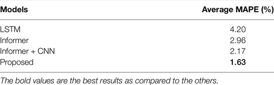
TABLE 1. Forecast results for the testing set of the GEFCom2014 data set.

3.2 Results of the North-American Utility Data Set

The proposed predictive model was performed on the testing set of the NAU data set. Its performance was compared with several models, including WT- NN Amjady and Keynia (2009), ESN Deihimi and Showkati (2012), SSA-SVR Ceperic et al. (2013), WT-ELM-MABC Li et al. (2015), CLPSO-MA-SVR Hu et al. (2014), WT-ELM-LM Li et al. (2016b), and ResNetPlus Chen et al. (2019). The results of these models are listed in Table 2. These comparative models have been proposed in the recent 10 years and cover feature selection, hyper-parameter optimization, DL, and other algorithms. Among these comparative models, the most recent proposed one, ResNetPlus, achieves an average MAPE value of 1.56%. Due to the advantages of learning long-sequence features and periodic load values, the proposed model achieves an average MAPE value of 1.15%, which is 1.35% and 0.34% lower than that of the traditional Informer and Informer + CNN models, respectively.

TABLE 2

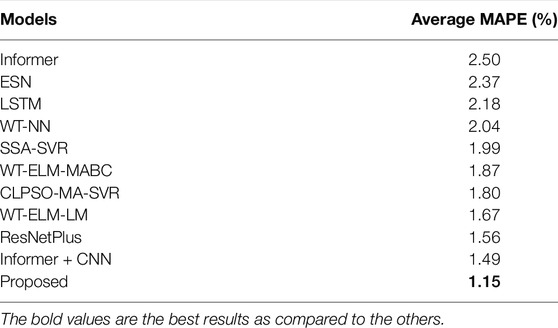
TABLE 2. Forecast results for the testing set of the North-American Utility data set.

3.3 Results of the ISO-NE Data Set

Two sets of prediction experiments were conducted for the ISO-NE data set. First, the proposed model was used to predict load profiles in 2006 and was compared with SIWNN Chen et al. (2010), WT-ELM-MABC Li et al. (2015), ResNetPlus Chen et al. (2019), and the traditional Informer models. Their results are showed in Table 3. The average MAPE value of every month is calculated respectively. The observation exists that the proposed model achieves lower average values than other models over 10 months, except for August and November. The overall average MAPE value of the proposed model is 0.57%, and it is 0.31%, 0.30%, 0.27%, and 1.88% lower than that of SIWNN, WT-ELM-MABC, ResNetPlus, and the traditional Informer models, respectively.

TABLE 3

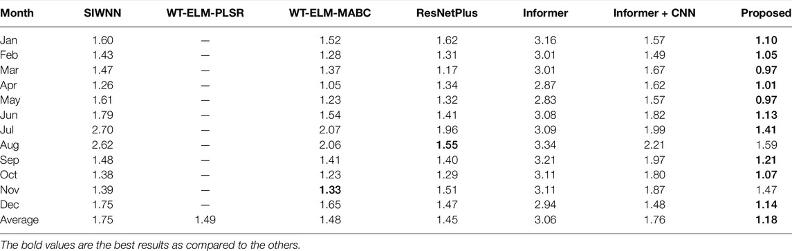
TABLE 3. Forecast results for the ISO-NE data set in the year 2006 (%).

The generalization capability of the proposed model was further tested on the data from 2010 and 2011. Table 4 reports the performance of the proposed model and five comparative models mentioned in Yu et al. (2014); Cecati et al. (2015); Li et al. (2016a); Chen et al. (2019). The observation exists that the proposed model achieves the best results as compared to other models. Compared to the traditional Informer and ResNetPlus models, the proposed model achieves lower mean MAPE values of 1.71% and 0.24% in 2010 and of 1.72% and 0.31% in 2011, respectively. It is worth noting that all of these models perform better in the year 2010 than in the year 2011. However, the traditional and the improved Informer models operate much more stable than others, as their difference values between the results of 2010 and 2011 are only 0.02% and 0.01%, respectively.

TABLE 4

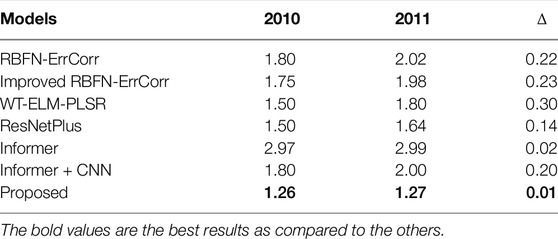
TABLE 4. Forecast results for the ISO-NE data set in 2010 and 2011 (%).

3.4 Robustness Analysis

The robustness of the proposed model to measuring errors was also tested. Same to some existing models, a set of normal Gaussian noise was added to the normalized temperature values. Tables 5–7 list the forecasting results of the three data sets by utilizing the normal and noisy data. Affected by the noisy data, the observation exists that the forecast performance of LSTM, Informer, and the proposed model decreases in all the three data sets. By using noisy data, the average MAPE values of the proposed model increase by 0.42% and 0.26% in the GEFCom2014 and NAU data sets, respectively. In 2006, 2010, and 2011 of the ISO-NE data set, the average MAPE values of the proposed model increase by 0.08%, 0.06%, and 0.05% respectively. Next, the Informer + CNN model is less affected by noisy data compared to LSTM and the proposed model. Take the GEFCom2014 data set as an example. The average MAPE value of the Informer + CNN model only increases by 0.05%, while the values of LSTM and the proposed model increase by 0.32% and 0.42%, respectively. It is worth noting that the traditional Informer model is not affected by the noisy data in some cases. For example, the average MAPE values of the traditional Informer model decrease by 0.34% and 0.78% in the GEFCom2014 and NAU data sets, respectively.

TABLE 5

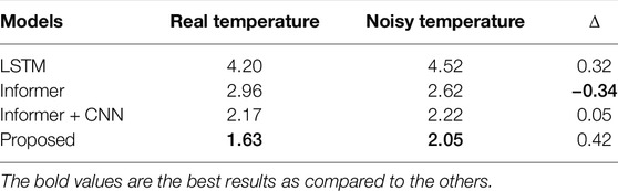
TABLE 5. Forecast results of the GEFCom2014 data set using real and noisy temperature data (%).

TABLE 6

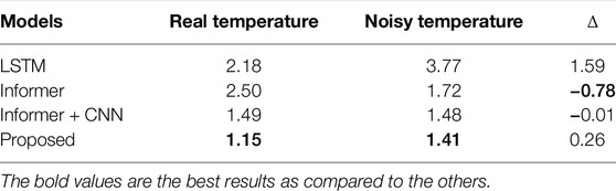
TABLE 6. Forecast results of the North-American Utility data set using real and noisy temperature data (%).

TABLE 7

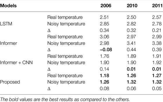
TABLE 7. Forecast results of the ISO-NE data set using real and noisy temperature data (%).

Compared with the traditional Informer model, the proposed model shows varying robustness to noisy temperature values on different data sets. The traditional Informer model is more robust to noisy temperatures than the proposed model on the GEFCom2014 and NAU data sets. On the contrary, the proposed model is better in 2010 and 2011 of the ISO-NE data set. Affected by noisy data, the average MAPE values of the traditional Informer model increase by 0.44% and 0.39%, respectively, while the average MAPE values of the proposed model increase only by 0.06% and 0.05%, respectively.

Figures 2–5 show the comparative box plots of LSTM, Informer, Informer + CNN, and the proposed model by real and noisy temperatures. Although the proposed model is affected by noisy data to some extent, it is still the best forecasting model in both cases.

FIGURE 2

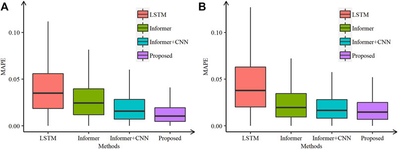
FIGURE 2. Comparative box plots of the proposed and other models in the GEFCom2014 data set using (A) real and (B) noisy temperatures.

FIGURE 3

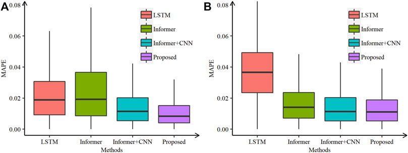
FIGURE 3. Comparative box plots of the proposed and other models in the NA data set using (A) real and (B) noisy temperatures.

FIGURE 4

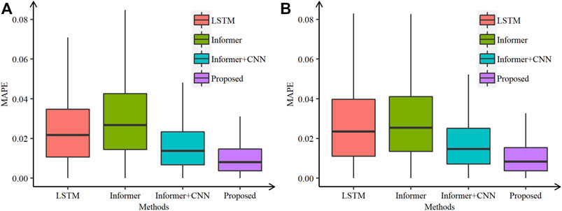
FIGURE 4. Comparative box plots of the proposed and other models in 2006 of the ISO-NE data set using (A) real and (B) noisy temperatures.

FIGURE 5

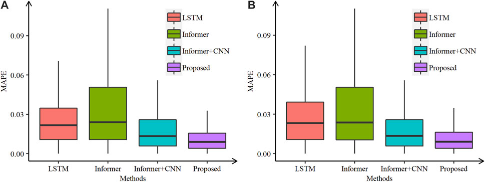
FIGURE 5. Comparative box plots of the proposed and other models in 2010 and 2011 of the ISO-NE data set using (A) real and (B) noisy temperatures.

3.5 Ablation Study

Additional experiments were also conducted on the three data sets with ablation consideration. All the experiments on the same data set were performed with the same hyper-parameters. Figure 6 shows the ablation results of the periodic values and CNN on the three data sets. It can be proved that the CNN module and the periodic load values demonstrate the ability to improve the predict performance in terms of MAPE.

FIGURE 6

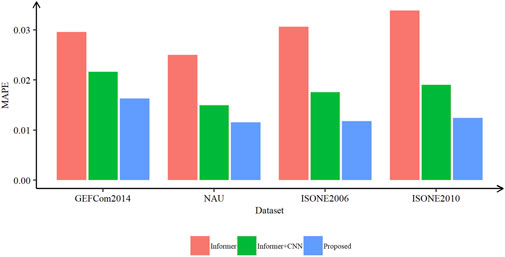
FIGURE 6. Predict results of the ablation of the proposed model on the three data sets.

3.6 Running Time

The Informer and the proposed model were performed on a Dell workstation with GPU installed. Table 8 lists the running times of every sequence during the training and the testing process. The results indicate several conclusions of interest. First, the training process consumes about three times as long as the testing process, which can be explained by the back-propagation of the training process. Second, the proposed model increases the complexity of the traditional Informer, and the increased percentages of running times in the testing process are greater than that in the training process.

TABLE 8

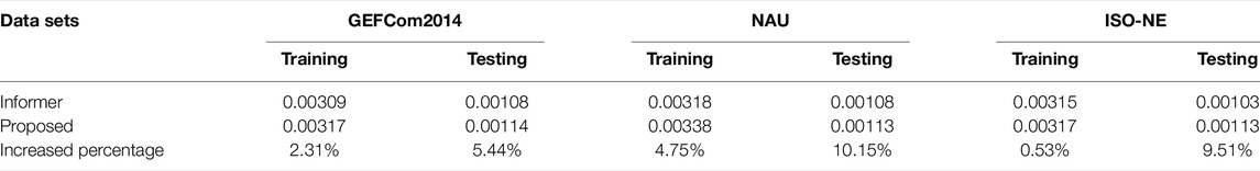
TABLE 8. Running time of the proposed model on the three data sets (s).

4 Conclusion

This paper proposes an improved Informer model for STLF. The traditional Informer model is improved by considering periodic load values of input load sequences. The performance of the proposed model was tested on three public data sets, and their results showed the superior forecasting ability of the proposed model as compared to not only the traditional Informer model but also other deep leaning based models.

Time-series forecasting has long been a research hotspot. The success of attention-based DL techniques promoted the development of this area. However, the performance of STLF needs further improvement. In our future work, we will try to improve the prediction accuracy by integrating some other techniques, such as clustering and ensemble strategy.

Data Availability Statement

The original contributions presented in the study are included in the article/Supplementary Material, further inquiries can be directed to the corresponding author.

Author Contributions

FL and YL contributed to conception and design of the study. TD organized the database. FL and TD performed the statistical analysis. FL, TD, and YL wrote the first draft of the manuscript. All authors contributed to manuscript revision, read, and approved the submitted version.

Funding

This work is financially supported by the Youth Science and Technology Talent Support Project of Jilin Province (QT202109), and the Science and technology Research Project of Education Department of Jilin Provincial (JJKH20221008KJ).

Conflict of Interest

TD was employed by the State Grid Jilin Electric Power Company Limited.

The remaining authors declare that the research was conducted in the absence of any commercial or financial relationships that could be construed as a potential conflict of interest.

Publisher’s Note

All claims expressed in this article are solely those of the authors and do not necessarily represent those of their affiliated organizations, or those of the publisher, the editors, and the reviewers. Any product that may be evaluated in this article, or claim that may be made by its manufacturer, is not guaranteed or endorsed by the publisher.

References

Amjady, N., and Keynia, F. (2009). Short-term Load Forecasting of Power Systems by Combination of Wavelet Transform and Neuro-Evolutionary Algorithm. Energy 34, 46–57. doi:10.1016/j.energy.2008.09.020

CrossRef Full Text | Google Scholar

Bedi, J., and Toshniwal, D. (2019). Deep Learning Framework to Forecast Electricity Demand. Appl. Energy 238, 1312–1326. doi:10.1016/j.apenergy.2019.01.113

CrossRef Full Text | Google Scholar

Cecati, C., Kolbusz, J., Rozycki, P., Siano, P., and Wilamowski, B. M. (2015). A Novel Rbf Training Algorithm for Short-Term Electric Load Forecasting and Comparative Studies. IEEE Trans. Ind. Electron. 62, 6519–6529. doi:10.1109/TIE.2015.2424399

CrossRef Full Text | Google Scholar

Ceperic, E., Ceperic, V., and Baric, A. (2013). A Strategy for Short-Term Load Forecasting by Support Vector Regression Machines. IEEE Trans. Power Syst. 28, 4356–4364. doi:10.1109/tpwrs.2013.2269803

CrossRef Full Text | Google Scholar

Chen, K., Chen, K., Wang, Q., He, Z., Hu, J., and He, J. (2019). Short-term Load Forecasting with Deep Residual Networks. IEEE Trans. Smart Grid 10, 3943–3952. doi:10.1109/Tsg.2018.2844307

CrossRef Full Text | Google Scholar

Chen, Y., Luh, P. B., Guan, C., Zhao, Y., Michel, L. D., Coolbeth, M. A., et al. (2010). Short-term Load Forecasting: Similar Day-Based Wavelet Neural Networks. IEEE Trans. Power Syst. 25, 322–330. doi:10.1109/TPWRS.2009.2030426

CrossRef Full Text | Google Scholar

Chicco, G., and Ilie, I.-S. (2009). Support Vector Clustering of Electrical Load Pattern Data. IEEE Trans. Power Syst. 24, 1619–1628. doi:10.1109/tpwrs.2009.2023009

CrossRef Full Text | Google Scholar

Deihimi, A., and Showkati, H. (2012). Application of Echo State Networks in Short-Term Electric Load Forecasting. Energy 39, 327–340. doi:10.1016/j.energy.2012.01.007

CrossRef Full Text | Google Scholar

Dumas, J., Wehenkel, A., Lanaspeze, D., Cornélusse, B., and Sutera, A. (2022). A Deep Generative Model for Probabilistic Energy Forecasting in Power Systems: Normalizing Flows. Appl. Energy 305, 117871. doi:10.1016/j.apenergy.2021.117871

CrossRef Full Text | Google Scholar

Hong, T., Pinson, P., Fan, S., Zareipour, H., Troccoli, A., and Hyndman, R. J. (2016). Probabilistic Energy Forecasting: Global Energy Forecasting Competition 2014 and beyond. Int. J. Forecast. 32, 896–913. doi:10.1016/j.ijforecast.2016.02.001

CrossRef Full Text | Google Scholar

Hu, Z., Bao, Y., and Xiong, T. (2014). Comprehensive Learning Particle Swarm Optimization Based Memetic Algorithm for Model Selection in Short-Term Load Forecasting Using Support Vector Regression. Appl. Soft Comput. 25, 15–25. doi:10.1016/j.asoc.2014.09.007

CrossRef Full Text | Google Scholar

Kong, W., Dong, Z. Y., Hill, D. J., Luo, F., and Xu, Y. (2018). Short-term Residential Load Forecasting Based on Resident Behaviour Learning. IEEE Trans. Power Syst. 33, 1087–1088. doi:10.1109/tpwrs.2017.2688178

CrossRef Full Text | Google Scholar

LeCun, Y., Bengio, Y., and Hinton, G. (2015). Deep Learning. Nature 521, 436–444. doi:10.1038/nature14539

PubMed Abstract | CrossRef Full Text | Google Scholar

Li, S., Goel, L., and Wang, P. (2016a). An Ensemble Approach for Short-Term Load Forecasting by Extreme Learning Machine. Appl. Energy 170, 22–29. doi:10.1016/j.apenergy.2016.02.114

CrossRef Full Text | Google Scholar

Li, S., Wang, P., and Goel, L. (2016b). A Novel Wavelet-Based Ensemble Method for Short-Term Load Forecasting with Hybrid Neural Networks and Feature Selection. IEEE Trans. Power Syst. 31, 1788–1798. doi:10.1109/tpwrs.2015.2438322

CrossRef Full Text | Google Scholar

Li, S., Wang, P., and Goel, L. (2015). Short-term Load Forecasting by Wavelet Transform and Evolutionary Extreme Learning Machine. Electr. Power Syst. Res. 122, 96–103. doi:10.1016/j.epsr.2015.01.002

CrossRef Full Text | Google Scholar

Ma, S. (2021). A Hybrid Deep Meta-Ensemble Networks with Application in Electric Utility Industry Load Forecasting. Inf. Sci. 544, 183–196. doi:10.1016/j.ins.2020.07.054

CrossRef Full Text | Google Scholar

Mashlakov, A., Kuronen, T., Lensu, L., Kaarna, A., and Honkapuro, S. (2021). Assessing the Performance of Deep Learning Models for Multivariate Probabilistic Energy Forecasting. Appl. Energy 285, 116405. doi:10.1016/j.apenergy.2020.116405

CrossRef Full Text | Google Scholar

Panapakidis, I. P. (2016). Application of Hybrid Computational Intelligence Models in Short-Term Bus Load Forecasting. Expert Syst. Appl. 54, 105–120. doi:10.1016/j.eswa.2016.01.034

CrossRef Full Text | Google Scholar

Sharda, S., Singh, M., and Sharma, K. (2021). A Complete Consumer Behaviour Learning Model for Real-Time Demand Response Implementation in Smart Grid. Appl. Intell. 52, 835–845. doi:10.1007/s10489-021-02501-4

CrossRef Full Text | Google Scholar

Shi, H., Xu, M., and Li, R. (2018). Deep Learning for Household Load Forecasting-A Novel Pooling Deep Rnn. IEEE Trans. Smart Grid 9, 5271–5280. doi:10.1109/Tsg.2017.2686012

CrossRef Full Text | Google Scholar

Sinha, A., Tayal, R., Vyas, A., Pandey, P., and Vyas, O. P. (2021). Forecasting Electricity Load with Hybrid Scalable Model Based on Stacked Non Linear Residual Approach. Front. Energy Res. 9. doi:10.3389/fenrg.2021.720406

CrossRef Full Text | Google Scholar

Ünal, F., Almalaq, A., and Ekici, S. (2021). A Novel Load Forecasting Approach Based on Smart Meter Data Using Advance Preprocessing and Hybrid Deep Learning. Appl. Sci. 11, 2742. doi:10.3390/app11062742

CrossRef Full Text | Google Scholar

Vaswani, A., Shazeer, N., Parmar, N., Uszkoreit, J., Jones, L., Gomez, A. N., et al. (2017). Attention Is All You Need.

Google Scholar

Wang, K., Qi, X., Liu, H., and Song, J. (2018). Deep Belief Network Based K-Means Cluster Approach for Short-Term Wind Power Forecasting. Energy 165, 840–852. doi:10.1016/j.energy.2018.09.118

CrossRef Full Text | Google Scholar

Yu, H., Reiner, P. D., Xie, T., Bartczak, T., and Wilamowski, B. M. (2014). An Incremental Design of Radial Basis Function Networks. IEEE Trans. Neural Netw. Learn. Syst. 25, 1793–1803. doi:10.1109/TNNLS.2013.2295813

PubMed Abstract | CrossRef Full Text | Google Scholar

Zahid, M., Ahmed, F., Javaid, N., Abbasi, R., Zainab Kazmi, H., Javaid, A., et al. (2019). Electricity Price and Load Forecasting Using Enhanced Convolutional Neural Network and Enhanced Support Vector Regression in Smart Grids. Electronics 8, 122. doi:10.3390/electronics8020122

CrossRef Full Text | Google Scholar

Zang, H., Xu, R., Cheng, L., Ding, T., Liu, L., Wei, Z., et al. (2021). Residential Load Forecasting Based on Lstm Fusing Self-Attention Mechanism with Pooling. Energy 229. doi:10.1016/j.energy.2021.120682

CrossRef Full Text | Google Scholar

Zhang, J., Zhang, H., Ding, S., and Zhang, X. (2021). Power Consumption Predicting and Anomaly Detection Based on Transformer and K-Means. Front. Energy Res. 9. doi:10.3389/fenrg.2021.779587

CrossRef Full Text | Google Scholar

Zhao, J., Huang, F., Lv, J., Duan, Y., Qin, Z., Li, G., et al. (2020). “Do rnn and Lstm Have Long Memory?,” in Proceedings of the 37th International Conference on Machine Learning.

Google Scholar

Zhou, H., Zhang, S., Peng, J., Zhang, S., Li, J., Xiong, H., et al. (2021). “Informer: Beyond Efficient Transformer for Long Sequence Time-Series Forecasting,” in Proceedings of AAAI.

Google Scholar