Bi-level deep reinforcement learning for PEV decision-making guidance by coordinating transportation-electrification coupled systems

The random charging and dynamic traveling behaviors of massive plug-in electric vehicles (PEVs) pose challenges to the efficient and safe operation of transportation-electrification coupled systems (TECSs). To realize real-time scheduling of urban PEV fleet charging demand, this paper proposes a PEV decision-making guidance (PEVDG) strategy based on the bi-level deep reinforcement learning, achieving the reduction of user charging costs while ensuring the stable operation of distribution networks (DNs). For the discrete time-series characteristics and the heterogeneity of decision actions, the FEVDG problem is duly decoupled into a bi-level finite Markov decision process, in which the upper-lower layers are used respectively for charging station (CS) recommendation and path navigation. Specifically, the upper-layer agent realizes the mapping relationship between the environment state and the optimal CS by perceiving the PEV charging requirements, CS equipment resources and DN operation conditions. And the action decision output of the upper-layer is embedded into the state space of the lower-layer agent. Meanwhile, the lower-level agent determines the optimal road segment for path navigation by capturing the real-time PEV state and the transportation network information. Further, two elaborate reward mechanisms are developed to motivate and penalize the decision-making learning of the dual agents. Then two extension mechanisms (i.e., dynamic adjustment of learning rates and adaptive selection of neural network units) are embedded into the Rainbow algorithm based on the DQN architecture, constructing a modified Rainbow algorithm as the solution to the concerned bi-level decision-making problem. The average rewards for the upper-lower levels are ¥ -90.64 and ¥ 13.24 respectively. The average equilibrium degree of the charging service and average charging cost are 0.96 and ¥ 42.45, respectively. Case studies are conducted within a practical urban zone with the TECS. Extensive experimental results show that the proposed methodology improves the generalization and learning ability of dual agents, and facilitates the collaborative operation of traffic and electrical networks.

1 Introduction

1.1 Motivation

Along with the emergence of new energy vehicles, plug-in electric vehicles (PEVs) gradually replace traditional gasoline vehicles (GVs) due to their ecologically-friendly and cost-efficient, becoming a promising opportunity for the future development of transportation and electrical industries. The global PEV sales and the number of public chargers are expected to reach 25 million and 11 million by 2030 (Luo et al., 2019), respectively, which would strengthen the interdependence between urban transportation networks (TNs) and power distribution networks (DNs) (Qi et al., 2022).

However, the surge of PEV penetration has lagged far behind the construction of charging infrastructure, leading to PEV charging issues, such as mileage anxiety, unanticipated charging congestion and high charging costs for owners. Besides, traveling routes and charging navigation in urban TNs face the difficulties, such as trip time uncertainty and mileage limitations (Xiang et al., 2022; Tu et al., 2020). Thus, the PEV decision-making guidance (PEVDG) in transportation-electrification coupled systems (TECSs) plays a critical role in enhancing the user charging experience and facilitating the collaborative operation of converged networks.

1.2 Literature survey

Until now, various efforts have been made to research PEV charging guidance strategies to optimize users’ decision-making behaviors. Reference (Wang et al., 2019) develops a geometry-based charging guidance strategy to recommend CSs for PEV motorists. It employs a Dijkstra algorithm to calculate the shortest straight-line distance between charging demand points and CSs, and assigns PEVs to the corresponding nearest CSs for recharging. Liu et al. (2019) propose a simplified charging control algorithm to reduce the traveling cost of owners via the joint optimization of en-route charging and routing.

Additionally, these studies (Wang et al., 2019; Kancharla et al., 2020; Morlock et al., 2020) focus on traveling time optimization in PEV charging navigation issues. Morlock et al. (2020) modify the Moore-Bellman-Ford algorithm and propose a two-stage model to recommend the shortest route. Reference (Kancharla et al., 2020) comprehensively considers navigation and charging time, and proposes an adaptive large neighborhood search algorithm to address the PEV non-linear charging and discharging. However, the work presented in (Wang et al., 2019) finds that the time-optimal strategy may lead to high exhaust emission and power consumption. It proposes an eco-routing model to reduce link energy costs by combining GVs and PEVs.

These scholars (Ji et al., 2020; Li et al., 2020) explore the feasibility of price-driven charging guidance strategies. Li et al. (2020) propose a price-incentive-based charging guidance strategy to solve simultaneous charging requirements. A specific time-sharing pricing strategy is formulated to reduce the PEV user’s average charging cost. Considering the interaction effect of the dynamic requirements of massive PEVs, research (Ji et al., 2020) establishes a dynamic reservation-waiting queuing model. To minimize the route distance, driving time and charging cost, this approach recommends the optimal CSs according to the order of PEV arrival time.

In studies (Luo et al., 2020; Shi et al., 2020; Sun et al., 2020), real-time interactive information from TECSs is exploited to help PEV owners make efficient charging decisions. For example, Reference (Luo et al., 2020) comprehensively considers the road speed of traffic networks, the congestion of CSs and the load of charging networks, and develops a PEV charging and battery swapping scheduling scheme. This solution can enhance the convenience of owners and relieve local traffic jams. Shi et al. (2020) capture the real-time response of PEV charging queuing to the traffic flow information via a point-type model, and propose an optimal decision for PEV fleets, including the route, departure time, and charging location. It effectively addresses the dynamic equilibrium of traffic flow caused by PEV aggregation for recharging. Based on the data fusion of the optimal power flow and the traffic flow assignment, Sun et al. (2020) develop a PEV integrated rapid-charging scheduling platform. The platform guides the vehicles to the most suitable CS for recharging under the constraint of coupled network nodes.

Further, studies (Sohet et al., 2021; Zhou et al., 2021) develop the PEV orderly decision-making to mitigate the impact of large-scale charging demand on traffic and electrical networks. Zhou et al. (2021) propose a hierarchical graph-theory-based weight model and apply the Dijkstra to search for the optimal decision-making scheme. Similarly, the TN condition and the DN load are converted respectively into the indicators of the time consumption of each road and the locational marginal price of each CS (Sohet et al., 2021). Although the above-mentioned solutions help us capture the nature of the PEVDG in the early stage, the conventional optimization works heavily rely on specific mathematical programming models, which still suffer from computational inefficiencies and poor solution quality. It is challenging to apply efficiently in a city-level transportation-electrification network.

Benefiting from the excellent approximation ability of deep neural networks (DNNs) (Duan et al., 2020), deep reinforcement learning (DRL) has received growing interest in the PEVDG field. References (Zhao et al., 2021; Yu et al., 2019) develop DNNs with different structures to solve the routing decision-making problem. In (Zhao et al., 2021), an actor-adaptive-critic-based DRL method is presented to minimize the tour length by specifying the next destination. To ease the computational burden, Yu et al. (2019) build a specific DNN for the PEV navigation, which takes traffic features and completed trips as the state and action, receptively.

Other scholars (Lee et al., 2020; Qian et al., 2020a; Zhang C. et al., 2021) introduce DRL into the CS recommendation field. The CS selection decision-making is transformed into a finite Markov decision process (FMDP) in (Lee et al., 2020), and the deep Q-network (DQN) is adopted to approximate the mapping relationship between the environmental state and the optimal CS with the shortest time consumption. Similarly, Zhang Y. et al. (2021) introduce different coefficients to balance the weight of total charging time and origin-destination distance, and adopt DQN to learn the recommended strategy. In (Qian et al., 2020b), the deterministic shortest charging route model is established to extract feature states, and DQN is employed to recommend CSs and corresponding routes to optimize the charging time and cost. Besides, considering the cooperative and competitive relationship among multiple decision makers, Reference (Zhang et al., 2022) regards each CS as an individual agent. The CS recommendation is constructed as a multi-objective and multi-agent reinforcement learning task. The agents explore and learn game policies among individuals to minimize the charging waiting time, charging cost and charging failure rate of PEV owners. Based on the multi-agent learning architecture, Reference (Wang et al., 2022) regards each electric taxi as an individual agent to formulate the charging or relocation recommendation strategy. The agents can maximize the cumulative profits of taxi drivers by learning non-cooperative game policies.

Further, these references (Lopez et al., 2019; Ding et al., 2020; Qian et al., 2020b) focus on formulating DRL-based PEV charging guidance schemes via complete interactive information of coupled systems, promoting the collaborative control of convergence networks. Karol et al. (Lopez et al., 2019) adopt a trained deep learning model to make optimal real-time decisions with knowledge of future energy prices and vehicle usage. Based on a deep deterministic policy gradient, Reference (Ding et al., 2020) proposes a multi-agent-based optimal PEV charging approach in a DN, and analyzes the impact of uncertainties on charging safety. Qian et al. (2020a) adopt a DRL-based optimization model to determine the CS pricing under the uncertainties of wind power output and traffic demand. It enhances the operation of the TECS and improves the integration of renewable energy by guiding PEV charging behaviors.

1.3 Research gap

A detailed comparison of the abovementioned literature is summarized in Table 1. There are still several significant limitations to the state-of-the-art PEVDG solutions in this field.

TABLE 1

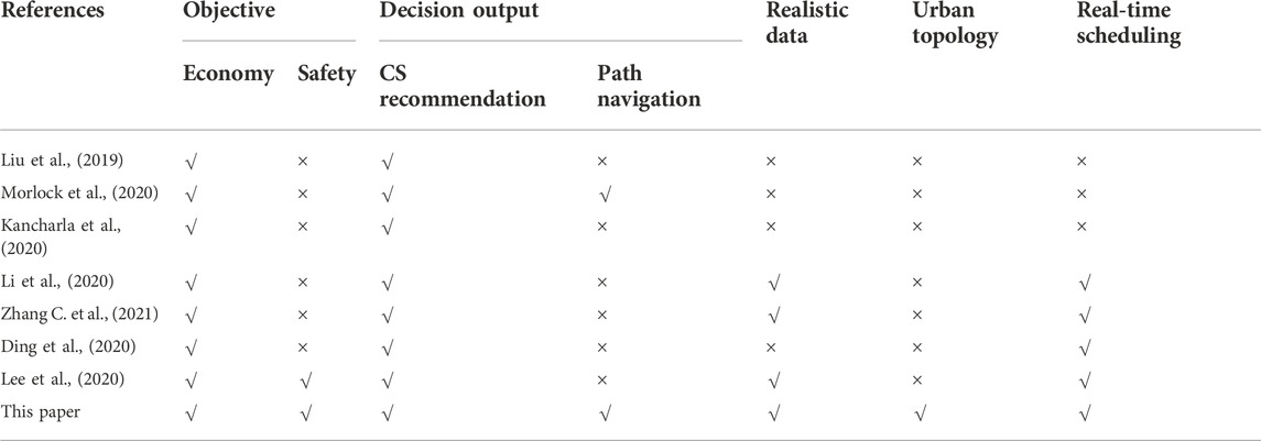
TABLE 1. Comparison of relevant literature.

For the offline-based PEVDG analytics, they use traditional dynamic programming (e.g., (Morlock et al., 2020), (Shi et al., 2020) and (Sun et al., 2020)) and heuristic search (e.g., (Wang et al., 2019), (Kancharla et al., 2020) and (Li et al., 2020)) for traffic segment planning and CS recommendation. Moreover, under the limited-scale traffic topology (e.g., (Liu et al., 2019), (Wang et al., 2019) and (Li et al., 2020)), most of them utilize a theoretical-modeling-based approach for scheduling and controlling PEVs, which lacks practical data support. In this way, it leads to low computational efficiency and unstable solution performance in city-size networks. In the complex dynamic coupled system with increasing PEV penetration, it is difficult to respond to the charging demand quickly.

For the DRL-based PEVDG analytics, they are widely adopted, benefiting from the real-time processing capability of discrete decision-making problems. However, due to the simple training and reward mechanisms, classical DQN methods (Lee et al., 2020) fail to coordinate the exploration speed and solution quality in the training phase. Moreover, they only adopt a single neural network for Q-value iterations, which may lead to inaccurate prediction results. As such, the classical DQN still suffers from the following deficiencies: Q-value estimation, stability performance, solution quality and generalization performance. In this way, agents often fail to output the optimal decision-making solution. Besides, due to its limited action output space, it is difficult for existing DRL-based optimization strategies to simultaneously solve the decision-making guidance problems of CS recommendation and path navigation (e.g., (Zhang C. et al., 2021), and (Ding et al., 2020)). Similarly, multi-agent-based DRL methods (e.g., (Zhang et al., 2022) and (Wang et al., 2022)) recommend the most appropriate CS to the owner, comprehensively considering the game influence among multiple decision makers. However, these methods output only homogeneous decision actions (i.e., charging or routing), without considering the interrelationship and influence of CS selection and path navigation. As such, it is challenging to make joint action decisions for PEVDG. In this way, the scalability and popularity of the DRL scheme in FEVDG are limited.

1.4 Contributions

To fill the gap, we consider the real-time mapping capability of the DRL-based approach for addressing complex decision-making problems. The heterogeneous decision-making actions of CS recommendation and path planning are reasonably coordinated and controlled. The traditional DQN-based method is improved as a solution to the decision-making problem. To this end, this paper proposes a novel bi-level DRL (namely, BDRL) scheme to tackle the PEVDG optimization issue. From the perspective of coordinated transportation-electrification operation, a comprehensive optimization objective is constructed to minimize the synthetic cost of PEV users in the TN while optimizing the voltage distribution of the DN. PEVDG is constructed as a bi-level FMDP (namely, BFMDP) model. A modified Rainbow-based DQN algorithm is developed as the solution for BFMDP. The main contributions of this paper are threefold.

(1) Given that the discrete decision-making process of PEVDG conforms to the Markov property, BFMDP is utilized to address the heterogeneous decision-making behaviors of charging and routing. The upper-level agent learns the CS recommendation decision and embeds the action output into the lower-level state space. The lower-level agent realizes the online path navigation decision output. The integrated output of charging-routing decisions is achieved through the coordination and cooperation of dual agents in the upper-lower levels, which improves the efficiency of PEVDG.

(2) Two extension mechanisms (i.e., learning rate decay and dropout layer technology) are embedded into the classical Rainbow to construct a modified Rainbow algorithm, improving the convergence performance, generalization ability and learning efficiency of the dual agents’ decision-making output. The learning rate of each episode is dynamically adjusted by an inverse decay model, balancing the quality of exploration in the early stage with the speed of exploitation in the later stage. The neural network units are selected adaptively in the training and testing stages to improve the shortcoming of over-fitting of traditional neural networks.

(3) Under the urban-level traffic topology framework, the proposed method is tested using real-world environmental data, realistically reflecting the owner’s charging willingness and reasonably providing decision-making support. The testing results show that BDRL reduces the overall cost of PEV users while ensuring the safe operation of converged charging networks.

1.5 Paper organization

The remainder of this paper is organized as follows. Section 2 sketches the modeling process of the PEVDG problem. Then our proposed modified Rainbow method is presented in Section 3. Case studies are reported in Section 4. Finally, Section 5 concludes the paper.

2 Problem modeling

Figure 1 illustrates the PEVDG architecture. Specifically, the decision-making of CS recommendation and path navigation is duly formulated as a BFMDP process. In the upper-level, CS recommendation is characterized as an optimal mapping of the state space of PEVs, CSs, and DNs to the charging resources. The agent determines the target CS action, which is also embedded into the state space of the lower-level agent. In doing so, the navigation target is determined for the routing. In the lower-level, PEV path navigation is characterized as an optimal mapping of the state space of PEVs and TNs to traffic road segments. The agent determines the traveling action by capturing real-time PEV status and TN information. Finally, a Modified Rainbow algorithm is proposed as a solution for the above-mentioned bi-level decision-making. Details of the modeling process and algorithm improvements are described as follows.

FIGURE 1

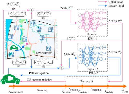
FIGURE 1. Overall scheme of our proposed PEVDG approach.

2.1 Mathematical formulation

We establish multiple-subject optimization to reduce the comprehensive cost of users and optimize the voltage deviation of DNs.

$f=\min \left[C_i^{\text{ec}}+C_i^{\text{ch}}+\varpi \left(T_i^{\text{tr}}+T_i^{\text{wt}}+T_i^{\text{ch}}\right)\right]+\min \left[\frac{1}{N^{\text{DN}}}{\displaystyle \sum }_{t=1}^T{\displaystyle \sum }_{k=1}^{N^{\text{DN}}}\left|\frac{V_{t,k}-V_k^{\ast }}{V_k^{\ast }}\right|\right](1)$

$C_i^{\text{ec}}={\overline{\pi }}^{\text{CS}}\mu {\displaystyle \sum }_{{\beta }_{mn}\in {\mathrm{\Omega }}_i}{d}_{mn}{\phi }_{mn}(2)$

$C_i^{\text{ch}}={\displaystyle \sum }_{t=t_i^{\text{sta}}}^{t_i^{\text{end}}}{\pi }_{j,t}^{\text{CS}}{P}^{\text{ch}}\Delta t(3)$

$T_i^{t\mathrm{r}}={\displaystyle \sum }_{{\beta }_{mn}\in {\mathrm{\Omega }}_i}\frac{d_{mn}{\phi }_{mn}}{{\overline{v}}_{mn}}(4)$

$T_i^{\text{ch}}=\frac{Q_i\left(e_i^{\exp }-e_i^{\text{arr}}\right)}{P^{\text{ch}}\eta }(5)$

where: $C_i^{\text{ec}}$ and $C_i^{\text{ch}}$ respectively indicate the energy consumption and charging cost of the ith PEV. $T_i^{\text{tr}}$, $T_i^{\text{wt}}$ and $T_i^{\text{ch}}$ respectively indicate the traveling, waiting, and charging time. $\varpi$ and $T$ respectively represent the cost per-unit time and the control time. $i\in {\mathrm{\Omega }}^{\text{EV}}$, ${\mathrm{\Omega }}^{\text{EV}}$ represent the set of PEVs. $V_{t,k}$ and $V_k^{\ast }$ respectively represent the real-time voltage and rated voltage. ${\mathrm{\Omega }}^{\text{DN}}$ indicates the set of DN nodes. ${\overline{\pi }}^{\text{CS}}$ is the average charging price of CSs. $\mu$ represents the energy consumption per kilometer. $d_{mn}$ denotes the length of the road segment ${\beta }_{mn}$ between the traffic nodes ${\beta }_m$ and ${\beta }_m$ in a TN $G^{\text{TN}}$. ${\beta }_m,{\beta }_n\in {\mathrm{\Omega }}^{\mathrm{E}}$, ${\mathrm{\Omega }}^{\mathrm{E}}$ is the set of road segments in a TN $G^{\text{TN}}$. ${\phi }_{mn}$ represents the binary variable for road segment selection. ${\mathrm{\Omega }}_i$ indicates the set of selected road segments for the ith PEV. ${\pi }_{j,t}^{\text{CS}}$ is the real-time charging price of the jth CS. $P^{\text{ch}}$ and $\eta$ respectively denote the output power and the efficiency of charging piles. Let $t_i^{\text{sta}}$ and $t_i^{\text{end}}$ respectively denote the starting and ending charging time. ${\overline{v}}_{mn}$ is the average traveling velocity of the road segment ${\beta }_{mn}$. $Q_i$ denotes the battery capacity. $e_i^{\text{arr}}$ and $e_i^{\mathit{exp}}$ respectively represent the state of charge (SOC) of the ith PEV arriving at the CS and the expected SOC of the ith PEV leaving the CS.

2.1.1 PEV constraints

$e_i^{\text{req}}-\frac{\mu {\displaystyle \sum }_{{\beta }_{mn}\in {\mathrm{\Omega }}_i}{d}_{mn}{\phi }_{mn}}{Q_i}>e^{\text{fl}}(6)$

${\displaystyle \sum }_{j\in {\mathrm{\Omega }}^{\text{CS}}}{\psi }_{i,j}=1(7)$

where: $e_i^{\text{req}}$ indicates the SOC of the triggered charging requirement. $e^{\text{fl}}$ represents the minimum SOC of the battery. If the SOC of a PEV is lower than the value of $e^{\text{fl}}$, it is considered to run out of energy en-route. ${\psi }_{i,j}$ is the binary variable for CS recommendation. ${\psi }_{i,j}=1$ means that the jth CS is recommended to the ith PEV, ${\psi }_{i,j}=0$ means not. ${\mathrm{\Omega }}^{\text{CS}}$ stands for the set of CSs. Note, Eq. 8 limits the energy range of PEVs.

2.1.2 Power flow constraints

$-P_{t,k}^{\text{cs}}-P_{t,k}^{\text{load}}=V_{t,k}{\displaystyle \sum }_{j\in k}{V}_{t,j}\left(G_{kj}\cos {\theta }_{t,kj}+B_{kj}\sin {\theta }_{t,kj}\right)(8)$

$-Q_{t,k}^{\text{cs}}-Q_{t,k}^{\text{load}}=V_{t,k}{\displaystyle \sum }_{j\in k}{V}_{t,j}\left(G_{kj}\sin {\theta }_{t,kj}-B_{kj}\cos {\theta }_{t,kj}\right)(9)$

where: $P_{t,k}^{\text{cs}}$ and $Q_{t,k}^{\text{cs}}$ are the active and reactive loads of the CS, respectively. $P_{t,k}^{\text{load}}$ and $Q_{t,k}^{\text{load}}$ represent the active and reactive conventional loads, respectively. $G_{ij}$ and $B_{ij}$ are branch conductance and susceptance, respectively. ${\theta }_{ij,t}$ is the phase angle difference.

2.1.3 Security constraints

During the grid operation, it is an important task to maintain the node voltage within a reasonable and controllable range. The large-scale aggregated charging behavior brings additional load to the DN nodes, which might make the node voltage to drop. Thus, the DN security constraints must be considered, as shown in Eqs 12, 13. Herein, $V_k^{\max }$ and $V_k^{\min }$ indicate the upper and lower boundaries of node voltage. $I_{kj}^{\max }$ and $I_{kj}^{\min }$ are the upper and lower limits of current, respectively.

$V_k^{\min }\le V_{t,k}\le V_k^{\max }(10)$

$I_{kj}^{\min }\le I_{kj,t}\le I_{kj}^{\max }(11)$

Notably, we use the topology with a reference voltage of 10.6 kV as the DN simulation environment. Thus, the upper and lower voltage limits are set to 0.95 and 1.05, respectively.

2.1.4 TN constraints

The TN model is the basis for the study of path planning. Thus, we introduce the graph-theoretic analysis method (Zhang Y. et al., 2021) to model and describe the urban TN G^TN. Figure 2 shows the topological structure of the TN.

FIGURE 2

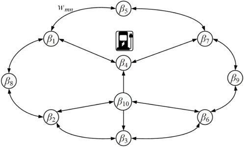
FIGURE 2. Topological structure of the TN.

From Figure 2, the two-way connecting arrows indicate two-way segments, and the one-way connecting arrows indicate one-way segments. β₄ indicates the geographical location of the CS in the TN. The modeling step for the given TN G^TN is described as follows.

$\{\begin{array}{l}{G}^{\text{TN}}=\left(B,E,W\right)\\ B=\left\{{\beta }_m|m=\mathrm{1,2,3},\dots ,{\mathrm{\Omega }}^{\mathrm{B}}\right\}\\ E=\left\{{\beta }_{mn}|{\beta }_m\in B,{\beta }_n\in B,m\ne n\right\}\\ W=\left\{w_{mn}|v_{mn}\in {\mathrm{\Omega }}^{\mathrm{E}}\right\}\end{array}(12)$

where: B denotes the set of all nodes of the graph, namely, the set of nodes of the TN G^TN. E denotes the set of all directed arc segments, namely, the set of road segments. W denotes the set of road segment weights, namely, the road resistances, indicating the quantitative attributes of road segments. Herein, the length of the road segment, traffic speed, traveling time, and traveling cost can be used as the road segment weight W for quantitative research.

Further, given a TN G^TN with ${\mathrm{\Omega }}^{\mathrm{B}}$ nodes for quantization assignment, the adjacent edge matrix $E_{mn}=a_{mn}$ is adopted to assign the road resistance to each road segment.

$a_{mn}=\{\begin{array}{l}{w}_{mn},\left(v_{mn}\in E\right)\\ 0,v_m=v_n\\ \infty ,\left(v_{mn}\notin E\right)\end{array}(13)$

The adjacent edge matrix E is expressed as follows:

$E=\left[\begin{array}{ccccc}0& w_{12}& w_{13}& \cdots & \infty \\ w_{21}& 0& w_{23}& \cdots & \infty \\ \infty & w_{32}& 0& \cdots & \infty \\ ⋮& ⋮& ⋮& \ddots & ⋮\\ \infty & \infty & \infty & \cdots & 0\end{array}\right](14)$

where: $\infty$ indicates that there is no connection segment between nodes $v_m$ and $v_n$.

Thus, a PEV owner performs optimal path planning by searching for the road segment resistance W. The topological constraints of the traveling path are expressed as follows.

${\displaystyle \sum }_{n=L_{t,i}^{\text{PEV}}}^{L_j^{\text{CS}}}{\phi }_{mn}-{\displaystyle \sum }_{n=L_{t,i}^{\text{PEV}}}^{L_j^{\text{CS}}}{\phi }_{nm}=\{\begin{array}{l}1m=L_{t,i}^{\text{PEV}}\\ 0m\ne L_{t,i}^{\text{PEV}},L_j^{\text{CS}}\\ -1m=L_j^{\text{CS}}\end{array}(15)$

where: the path from the current location $L_{t,i}^{\text{PEV}}$ to the location of the assigned CS $L_j^{\text{CS}}$ is planned according to the starting, the intermediate and the ending nodes. In doing so, it is ensured that the selected segments can be connected sequentially.

2.2 Formulation of BFMDP-based PEVDG

Reinforcement learning means that the agent perceives the environmental information and obtains the rewards by the trial and error strategy. Then the agent selects an action to execute according to the current environment state. The environment is converted to a new state. The environment perception is repeated to obtain state rewards and action outputs until the end of the control process. In this way, the agent establishes the optimal mapping relationship between states and actions through repeated trial and error. Moreover, the change of the next state in reinforcement learning is only related to the current state and the action selected by the agent, but not related to the previous state, that is, the process satisfies Markovian properties. Such reinforcement learning that satisfies Markovian properties is defined as an FMDP (Lee et al., 2020).

As for PEVDG with multi-subject interaction and multi-objective optimization, the PEV owner, as the agent, perceives the transportation-electrification environment information, including the road status, charging price and charging cost. By comprehensively evaluating the reward obtained from the current charging and traveling states, the agent selects successively the appropriate CS for energy supply and the optimal traveling path for navigation, until the action is completed and the destination is reached. Thus, the decision-making process of PEVDG fully conforms to the relevant definition of the FMDP.

Accordingly, FMDP is a typical model for depicting time-series decision-making problems, which is widely used in DN control (Alqahtani et al., 2022), energy dispatch (Hessel et al., 2017), and other fields. However, CS recommendation and path navigation are distinctly different time-scale scheduling problems. To this end, we propose a multi-time scale BFMDP to decouple the CS recommendation and path selection and reduce the dimension of the scheduling model.

2.2.1 States

The state represents the real-time perception of environment information by the agent, and the state space represents the set of environment information.

2.2.1.1 Upper-level for CS recommendation

Considering that the essence of CS recommendation is the spatio-temporal matching process between PEV charging requirements and CS energy resources, we divide the upper-level state $s_i^{\text{upp}}$ into real-time PEV, CS and DN information.

$s_i^{\text{upp}}=\left\{\underset{\text{PEV}}{\underbrace{t,e_{t,i}^{\text{PEV}},L_{t,i}^{\text{PEV}}}},\underset{\text{CS}}{\underbrace{{\pi }_{t,j}^{\text{CS}},{\xi }_{t,j}^{\text{CS}},L_j^{\text{CS}}}},\underset{\text{DN}}{\underbrace{P_{t,k}^{\text{DN}},V_{t,k}^{\text{DN}}}}\right\},\forall i\in {\mathrm{\Omega }}^{\text{PEV}},j\in {\mathrm{\Omega }}^{\text{CS}},\forall k\in {\mathrm{\Omega }}^{\text{DN}}(16)$

where: $e_{t,i}^{\text{PEV}}$ indicates the real-time SOC of the ith PEV, which is equal to $e_i^{\text{req}}$ in the upper-level. $L_{t,i}^{\text{EV}}$ represents the current location of the ith PEV. ${\xi }_{t,j}^{\text{CS}}$ is the state variable of the jth CS. If ${\xi }_{t,j}^{\text{CS}}\ge 0$, represents the number of idle piles, otherwise, represents the number of queuing users. $L_j^{\text{CS}}$ is the location of the jth CS. $P_{t,k}^{\text{DN}}$ and $V_{t,k}^{\text{DN}}$ indicate the active power load and the DN voltage.

2.2.1.2 Lower-level for path navigation

Once receiving the target CS output from the upper-level, the lower-level agent navigates toward the destination (namely, the target CS). Thus, the lower-level state $s_{i,t}^{\text{low}}$ can be expressed as below.

$s_{i,t}^{\text{low}}=\left\{\underset{\text{PEV}}{\underbrace{t,e_{t,i}^{\text{PEV}},L_{t,i}^{\text{PEV}}}},\underset{\text{TN}}{\underbrace{L_{i,j}^{\text{target}},{\overline{v}}_{mn},d_{mn}}}\right\},\forall i\in {\mathrm{\Omega }}^{\text{PEV}},\forall m,n\in {\mathrm{\Omega }}^{\text{TN}}(17)$

where: $L_i^{\text{target}}$ denotes the location of the target CS.

2.2.2 Actions

The action indicates a decision made by the agent in a given environment state.

2.2.2.1 Upper-level for CS recommendation

The action output from the upper-level is defined as the index of the recommended CS, as expressed in Eq. 20.

$a_i^{\text{upp}}=\left\{L_j^{\text{CS}}\right\},j\in {\mathrm{\Omega }}^{\text{CS}}(18)$

2.2.2.2 Lower-level for path navigation

Given a traffic network $G^{\text{TN}}$, the PEV path navigation decision-making is a discrete road segment selection problem. The lower-level action $a_{t,i}^{\text{low}}$ can be expressed as below:

$a_{t,i}^{\text{low}}=\left\{{\beta }_{\varphi }\right\},{\beta }_{\varphi }\in {\mathrm{\Omega }}_{t,i}^{\text{road}}(19)$

where: ${\mathrm{\Omega }}_{t,i}^{\text{road}}$ stands for the set of traffic nodes connected to the current location of the ith PEV $L_{t,i}^{\text{PEV}}$. That is, the road segment of the TN is used as the action of the lower-level agent. The obtained series of decision-making actions are connected sequentially to construct the optimal navigation path ${\psi }_{t,i}^{\text{low}}$. The PEV travels along the path ${\psi }_{t,i}^{\text{low}}$ from the current location $L_{t,i}^{\text{PEV}}$ until it reaches the location of the target CS $L_j^{\text{CS}}$.

${\psi }_{t,i}^{l\text{ow}}={\sum }_{L_{t,i}^{\text{EV}}}^{L_j^{\text{CS}}}{a}_{t,i}^{\text{low}}(20)$

2.2.3 Rewards

The reward indicates timely feedback obtained by the agent after performing an action.

2.2.3.1 Upper-level for CS recommendation

In the upper-level, the action selection directly affects the charging cost $C_i^{\text{ch}}$, waiting time $T_i^{\text{wt}}$, and charging time $T_i^{\text{ch}}$ after the user arrives at the CS. Meanwhile, the charging decisions of large-scale PEVs would affect the DN operation state. The upper-level reward is expressed as below.

$r_i^{\text{upp}}=-C_i^{\text{ch}}-\omega \left(T_i^{\text{wt}}+T_i^{\text{ch}}\right)-\frac{{\varpi }^{\text{sp}}}{N^{\text{DN}}}{\displaystyle \sum }_{k=1}^{N^{\text{DN}}}\left|\frac{V_{t,k}-V_k^{\ast }}{V_k^{\ast }}\right|(21)$

where: ${\varpi }^{\text{sp}}$ stands for the safety penalty.

2.2.3.2 Lower-level for path navigation

Combining the optimization goal and the reward obtained from the upper-level, we design the lower-level reward, including the energy consumption cost and traveling time cost. Once the PEV reaches the target CS $L_{i,j}^{\text{target}}$, the lower-level agent receives a positive reward. Conversely, if the PEV does not reach its destination before the battery runs out en-route, the user will need to request a towing rescue service. In this case, the agent obtains a negative punishment. As such, the lower-level reward is taken as the road resistance $w_{mn}$ of the TN G^TN, and assigned to each road segment. The agent determines the current action by comparing the feedback of rewards or punishments generated by the road resistance $w_{mn}$.

$w_{mn}=r_{t,i}^{\text{low}}=\{\begin{array}{l}-d_{mn}{\phi }_{mn}{\overline{\pi }}^{\text{CS}}\mu +\frac{\omega d_{mn}{\phi }_{mn}}{{\overline{v}}_{mn}},L_{t+1,i}^{\text{PEV}}\ne L_{i,j}^{\text{target}}\\ {\omega }^{\text{arr}},L_{t+1,i}^{\text{PEV}}=L_{i,j}^{\text{target}}\\ -{\omega }^{\text{tow}},e_{t,i}^{\text{EV}}-\frac{\mu d_{mn}{\phi }_{mn}}{Q_i}<e^{\text{flat}}\end{array}(22)$

where: the next location $L_{i,t+1}^{\text{PEV}}$ is determined by the current location $L_{t,i}^{\text{PEV}}$ and the road segment selection action $a_{t,i}^{\text{low}}$. ${\omega }^{\text{arr}}$ represents the reward for successfully reaching the target CS $L_{i,j}^{\text{target}}$. $-{\omega }^{\text{tow}}$ represents the penalty for navigation failure(namely, the average towing cost).

2.2.4 State action value function

After performing a specific action, the state-action value function (Q-value) evaluates the cumulative expected rewards that can be obtained by relying on the current policy $\psi$. Although upper-lower agents depend on the policies ${\psi }^{\text{upp}}$ and ${\psi }^{\text{low}}$, their Q-values $Q^{\psi }\left(s,a\right)$ can be expressed uniformly using the following equation.

$Q^{\psi }\left(s,a\right)=\mathbb{E}\left[{\displaystyle \sum }_{h=0}^H{\gamma }^h{r}_{t+h}|s_t=s,a_t=a\right](23)$

where: H indicates the horizon of the time steps. $\gamma$ indicates the discount factor.

Further, the purpose of the PEVDG problem is to find the optimal policy over all feasible policies, which is equivalent to finding the policy that can obtain the maximum $Q^{\pi }\left(s,a\right)$.

$Q^{\psi \ast }\left(s,a\right)=\underset{\psi }{\max }{Q}^{\psi }\left(s,a\right)(24)$

3 Proposed modified rainbow algorithm

3.1 Extension improvement mechanism

The classical DQN method has shown powerful ability in solving time-series decision-making problems. However, the classical DQN method uses a single deep network for function approximation and maximum Q-value for fitting estimation. In practical applications, there are still the following shortcomings, such as generalization, learning ability, computing efficiency and convergence performance. To address the above-mentioned issues, we introduce a modified DQN version-Rainbow algorithm into PEVDG.

The classical Rainbow (Qian et al., 2020a), as a DQN-based architecture, provides the possibility of integrating various complementary extension mechanisms. It means that users can independently add specific extensions to the basic DQN for different application scenarios, improving the algorithm’s learning ability and decision-making performance.

The classical Rainbow algorithm combines excellent mechanisms of Double DQN, Dueling DQN and the prioritized replay buffer. Further, we add two specific improvement mechanisms (i.e., the learning rate decay and the dropout layer technology) to form a modified Rainbow algorithm. The architecture is shown in Figure 3. Specifically, the learning rate decay mechanism dynamically adjusts the learning rate at each episode to improve the learning performance of the dual agents for environmental exploration. The dropout layer technology adaptively selects and discards neural network units in the training and testing phases, preventing the network from over-fitting and improving the generalization performance of the algorithm.

FIGURE 3

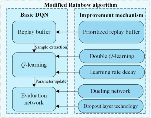
FIGURE 3. Architecture of the modified Rainbow algorithm.

3.1.1 Double DQN

For basic DQN, the maximum Q-value is utilized for iterative updates, which causes the Q-value overestimation. Thus, Double DQN changes the iteration rule of Q-value as shown in Equation. (27).

$Q\left(s_t,a_t;{\theta }^{+}\right)=Q\left(s_t,a_t;{\theta }^{+}\right)+\alpha \left[r_t+\gamma Q\left(s_{t+1},\underset{a^{\prime }}{\mathrm{a}\mathrm{r}\mathrm{g}\mathrm{m}\mathrm{a}\mathrm{x}}Q\left(s_{t+1},a^{\prime };{\theta }^{+}\right);{\theta }^{-}\right)-Q\left(s_t,a_t;{\theta }^{+}\right)\right](25)$

where: ${\theta }^{+}$ and ${\theta }^{-}$ are parameters of the evaluation network and target network, respectively. $\alpha$ indicates the learning rate.

3.1.2 Dueling DQN

Dueling DQN outputs the Q-value by dividing the network structure into the state value $V\left(s_t\right)$ and action advantage $A\left(s_t,a_t\right)$. The change of network structure removes redundant degrees of freedom and improves the efficiency of the algorithm.

$Q\left(s_t,a_t\right)=\mathfrak{V}\left(s_t\right)+\left[A\left(s_t,a_t\right)-\frac{1}{\left|A\right|}\right]{\displaystyle \sum }_{a^{\prime }\in A}A\left(s_t,a^{\prime }\right)(26)$

where: $\left|A\right|$ is the number of actions in action space A.

3.1.3 Prioritized replay buffer

In the training stage, the prioritized replay buffer specifies the sampling probability of all transitions based on the time difference error (TD-error). In this way, those samples with larger TD-error are extracted with a higher probability for network parameter optimization, which improves the computability and convergence of training.

${\delta }_j=r_j+\gamma Q\left[s_{j+1},\underset{a^{\prime }}{\mathrm{a}\mathrm{r}\mathrm{g}\mathrm{m}\mathrm{a}\mathrm{x}}Q\left(s_{j+1},a^{\prime };{\theta }^{+}\right);{\theta }^{-}\right]-Q\left(s_j,a_j;{\theta }^{+}\right)(27)$

$p_j=\frac{1}{\text{rank}\left(j\right)}(28)$

where: ${\delta }_j$ denotes the TD-error of the jth transition. $\text{rank}\left(j\right)$ represents the loss sorting. $p_j$ denotes the probability that the transition is stored into the mini-batch.

3.1.4 Learning rate decay

The learning rate is reduced based on the inverse time decay model to balance early exploration and later utilization. The learning rate ${\alpha }_n$ of the agent in each episode can be expressed as below.

${\alpha }_n={\alpha }^0{\left(1+\tau \frac{n}{n^d}\right)}^{-1}(29)$

where: ${\alpha }^0$ is the initial learning rate. $\tau$ denotes the decay coefficient. $n$ and $n^{\mathrm{d}}$ receptively represent the current episode and decay episode.

3.1.5 Dropout layer technology

Deep neural networks with many parameters are a powerful machine learning system. However, over-fitting and low computational performance are disadvantages during training and testing. Thus, the dropout layer technology can effectively alleviate the over-fitting of the evaluation network to the training data and improve the generalization ability and processing efficiency (Srivastava et al., 2014).

For a neural network with L layers, let $l\in \left\{1,...,L\right\}$ index the hidden layers. $w$, $b$ and $x$ denote the weights, biases, and inputs at the lth layer, respectively.

In the training stage, the output ${\stackrel{\sim }{y}}^l$ of the feed-forward neural network with dropout is represented as follows:

${\stackrel{\sim }{y}}^l=f\left(w^l{x}^l+b^l\right)\otimes {\mu }^l,{\mu }^l\sim B\left(1-p\right)(30)$

where: $\otimes$ denotes an element-wise product. For any layer l, ${\mu }^l$ is a vector of independent Bernoulli random variables. $p$ denotes the dropout probability.

In the testing stage, the output ${\widehat{y}}^l$ of the feed-forward neural network with dropout is represented as follows:

${\widehat{y}}^l=\left(1-p\right)f\left(w^l{x}^l+b^l\right)(31)$

3.2 Training process of BDRL

The flowchart and training process of the proposed solution are shown in Figure 4 and Table 2, respectively. In each episode, the upper-level agent first observes the environmental state $s_i^{\text{upp}}$ of PEVs, CSs and DNs. and selects a target CS $a_i^{\text{upp}}$ based on the evaluation network. The target CS is also embedded into the state space $s_{t,i}^{l\text{ow}}$ of the lower-level agent. Then the lower-level agent receives the upper-level navigation target and formulates the road segment selection schemes. After executing the action $a_{t,i}^{\text{low}}$, the lower-level agent obtains the corresponding reward $r_{t,i}^{\text{low}}$. The transition $\left(s_{i,j}^2,a_{i,j}^2,r_{i,j}^2,s_{i,j+1}^2\right)$ is stored in the replay buffer D. Next, a mini-batch is extracted via the prioritized replay buffer to update the network parameters. Finally, once the PEV arrives at the target CS, the corresponding reward of the upper-level agent is calculated $r_i^{\text{upp}}$. The upper-level network is updated in the same way as the lower-level. Especially, the learning rate ${\alpha }_n$ is decayed with the increase of episodes. The above steps are repeated until the maximum episode $N^{\text{epi}}$.

FIGURE 4

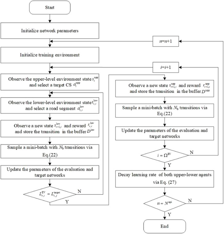
FIGURE 4. Flowchart of the proposed solution.

TABLE 2

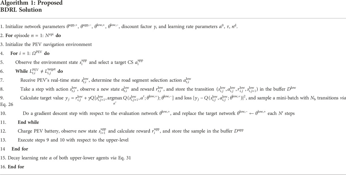
TABLE 2. Training process of the proposed BDRL Solution.

4 Case studies

4.1 Case study setup

In this study, the experimental setup of the “EV-CS-TN-DN” is shown in Figure 5. The performance of our proposed method is illustrated within a real-world TN in Nanjing, as shown in Figure 6. Wherein, nine blue nodes are CSs equipped with ten charging piles. The output power of charging piles is 60 kW. The IEEE 33-bus distribution system is adapted to match the size of the TN. The CSs are connected to DN nodes 4, 6, 9, 13, 16, 20, 24, 28, and 32, respectively. A total of 1000 PEVs with a battery capacity of 40 kWh need to be charged daily in this zone, and the triggered charging requirement SOC obeys $\mathcal{N}\left(3.2,{0.48}^2\right)$.

FIGURE 5

FIGURE 5. Experimental setup of the ‘EV-CS-TN-DN’.

FIGURE 6

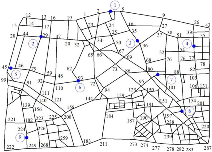
FIGURE 6. Topology of TNs and the location of CSs.

In the upper-level, the charging price is determined by the time of use (TOU) price [10], the cost per-unit time $\varpi$ is set as 86.02 ¥/h (Hu et al., 2019), and the energy consumption coefficient is 0.2 kWh/km (Zou et al., 2016). The safety penalty ${\varpi }^{\text{sp}}$ is set as ¥100. In the lower-level, the success reward and failure penalty for PEV guidance are set as ¥100 and ¥200, respectively. The minimum SOC of PEVs is 0.05. Besides, Table 3 lists the parameter of the modified Rainbow algorithm. All experiments are implemented in a server with CPU R93950X, GPU RTX3080TI and RAM 32GB.

TABLE 3

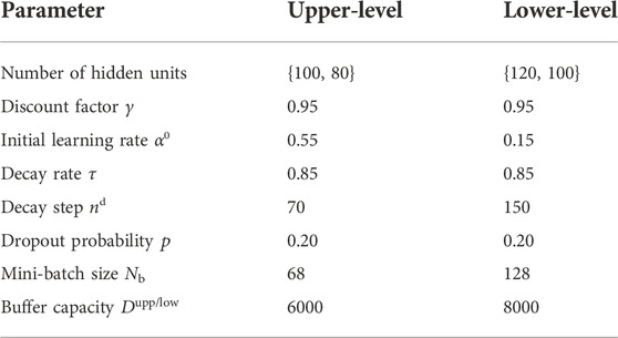
TABLE 3. Parameter of the modified Rainbow algorithm.

Herein, the decision-making complexity of road segment selection is significantly larger than that of CS selection. Thus, compared with the upper-level agent, the lower initial learning rate α⁰ and the decay step n^d are set in the lower-level agent. In this way, the lower-level agent explores more feasible schemes with a smaller learning rate in each episode, preventing the dilemma of local optimization. Besides, since the number of decision-making actions of the lower-level agent is much larger than that of the upper-level agent, the lower-level agent needs a larger mini-batch size and buffer capacity. In this way, the correlation of the samples can be effectively reduced.

4.2 Training process

Figures 7, 8 illustrates the reward for each training episode. The total training duration over 1000 episodes takes 4.25 h. As depicted, agents are encouraged to explore the environment with a large learning rate in the early stage, and the rewards fluctuate significantly. By accumulating historical experience, the upper-level agent learns to recommend the optimal CS and achieves convergence after 200 episodes, with an average reward with ¥ -90.64. As shown in Figure 8, however, the lower-level agent is stable only after about 450 episodes due to the complex traffic environment and the unstable upper-level output. Specifically, in the first 200 episodes, the lower-level agent is not competent for the guidance task, resulting in the battery depletion of several PEVs. With the increase in training episodes, the rewards obtained by the lower-level agent finally stabilized at about ¥ 13.24. The dual agents coordinate and cooperate to achieve the charging and routing decision-making guidance for PEV users.

FIGURE 7

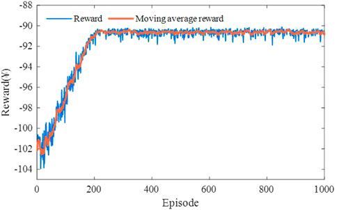
FIGURE 7. Training process of the upper-level agent for the proposed BDRL method.

FIGURE 8

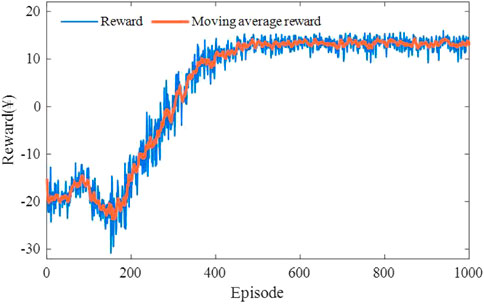
FIGURE 8. Training process of the lower-level agent for the proposed BDRL method.

4.3 Practical testing results

To compare with the proposed BDRL method, we use the offline disordered decision-making guidance method (DDG) as a baseline. That is, the upper-level CS recommendation decision selects a CS with the nearest to the charging trigger location. And the lower-level path navigation decision uses a path planning strategy (e.g., Dijkstra) to select the shortest traveling segments. The path navigation result and the total user cost are shown in Figures 9, 10, respectively. From Figure 9, we choose the path planning results between traffic node 91 and CS node 7 for illustration and comparsion. To weigh the traveling time and energy consumption, the agent provides four routes for PEV users during the peak hours from 17:00 to 19:00, excluding Path-1. Due to ideal traffic conditions, the agent recommends three paths, including Path-1 from 13:00 to 15:00. Thus, the proposed method can be adaptively adjusted according to dynamic traffic information to meet real-time traffic path planning requirements.

FIGURE 9

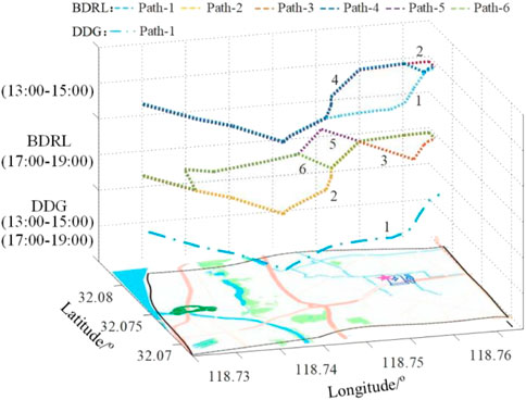
FIGURE 9. Path navigation results for BDRL and DDG methods under different periods.

FIGURE 10

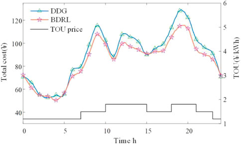
FIGURE 10. Total user cost for BDRL and DDG methods under different periods.

Besides, it can be seen from Figure 10 that the average total cost for users is ¥ 90.46 and the cost reaches ¥ 120.41 from 18:00 to 21:00 under the disordered guidance method. However, depending on the collaboration of dual agents, BDRL can effectively perceive the changes in the TOU electricity price and traffic information and optimize the decision-making scheme. The average cost for users is only ¥ 109.63 from 18:00 to 21:00, and the average daily cost is ¥ 85.43, which is 5.56% lower than the disordered guidance method.

To evaluate the impact of PEV aggregation charging on regional load operators, the spatial-temporal distribution of charging loads for CSs is shown in Figures 11, 12. Obviously, recharging customers are mainly concentrated at CSs 7 and 8 via the disordered guidance method, whereas CSs 1, 2 and 5 have fewer recharging customers. Conversely, BDRL effectively smoothes the charging load at each CS.

FIGURE 11

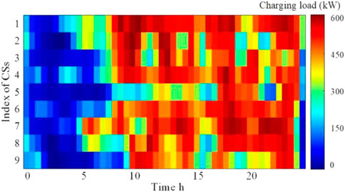
FIGURE 11. Spatial-temporal distribution of charging loads for CSs using the DDG method.

FIGURE 12

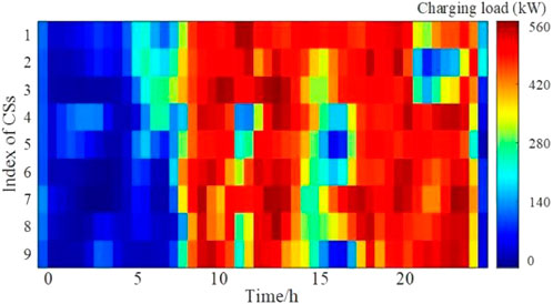
FIGURE 12. Spatial-temporal distribution of charging loads for CSs using the BDRL method.

Besides, we establish the equilibrium degree of the charging service $D^{\mathrm{e}}$, as shown in Eq. 34, to further quantify the service level of CSs. Herein, $D^{\mathrm{e}}$ denotes the equilibrium degree of charging service. $N_j^{\text{PEV}}$ denotes the number of PEVs served by the jth CS. ${\overline{N}}^{\text{PEV}}$ denotes the average number of PEVs at all CSs.

$D^{\mathrm{e}}=\sqrt{\frac{1}{{\mathrm{\Omega }}^{\text{CS}}}{{\displaystyle \sum }_{j\in {\mathrm{\Omega }}^{\text{CS}}}\left(N_j^{\text{PEV}}-{\overline{N}}^{\text{PEV}}\right)}^2}(32)$

The equilibrium degrees $D^{\mathrm{e}}$ under the disordered guidance method and our proposed method are 1.39 and 0.98, respectively. It indicates that BDRL optimizes the real-time matching of charging resources with charging demand. With the increase in PEV penetration, BDRL can provide PEV users with a better charging experience with limited charging resources.

Further, we also evaluate the impact of PEV aggregation charging on the DN. Figure 13 shows the node voltage distribution of the DN at 20:00 for different methods. For the DDG method, the random charging behavior of PEVs leads to load aggregation at several CSs, which increases the DN operational burden. For example, the voltage violation occurs at both nodes 18 and 33 at the end of the line, and the voltage qualification rate is only 72.73%. In contrast, BDRL coordinates the charging behavior of PEVs through a bi-level strategy, effectively balancing the regional load without voltage violations.

FIGURE 13

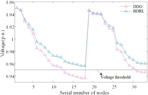
FIGURE 13. Node voltage distribution at 20:00 for DDG and BDRL methods.

4.4 Generalization ability analysis

In this part, we design new training scenarios to analyze the BDRL’s generalization ability. Specifically, we assume that CSs 1, 6, and 8 serve 400 PEVs daily, and the average charging price of the CSs changes in episodes 301 and 601, respectively. Figure 14 exhibits the reward distribution of the upper-level agent in three scenarios. Besides, the basic DQN method is taken as a baseline for comparison. Figure 15 shows the users’ average charging costs for the basic DQN and BDRL methods.

FIGURE 14

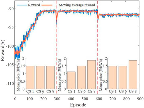
FIGURE 14. Training process of the upper-level agent under the CS charging price change scenarios.

FIGURE 15

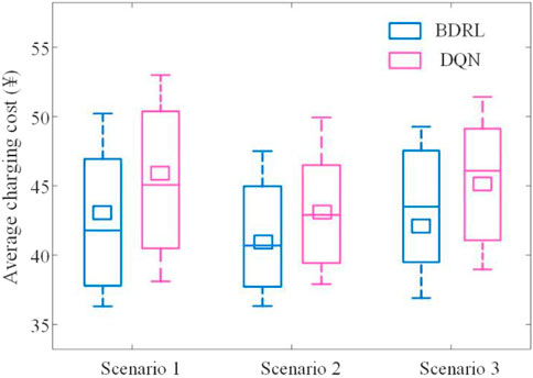
FIGURE 15. Average charging cost of users under the CS price change scenarios.

As depicted by Figures 14, 15, both sudden changes in environment information make the rewards drop sharply. Nonetheless, the agent adjusts the action output in time and achieves rapid convergence in several episodes by perceiving the reward changes. The average rewards for the three scenarios are ¥ -94.76, ¥ -90.88, and ¥ -91.80, respectively. Besides, the average charging costs under the three scenarios are ¥ 43.34, ¥ 41.41, and ¥ 42.13, respectively. This is because BDRL uses the dropout layer technology to adaptively select and discard the corresponding neural network units in the training and testing stages, which enables the well-trained fully connected networks to effectively identify and track environment changes. Conversely, the basic DQN without dropout layer units, the neural network layer cannot capture environmental changes in real-time for effective mapping output. For the basic DQN, the user charging cost increases by 5.72%, 4.20%, and 7.00% under the three scenarios, respectively. Overall, it is shown that the proposed method can quickly adapt to untrained scenarios and has the ability to generalize to data outside the training set.

4.5 Numerical comparison with comprehensive methods

Finally, we choose an offline strategy (namely, DDG) as well as traditional DRL strategies (namely, DQN, Double-DQN and Dueling-DQN) to comprehensively compare the implementation effectiveness of BDRL. Specifically, we use DQN, Double-DQN and Dueling-DQN as the solutions for the BFMDP, which also undergo 1000 training episodes. The training time for offline and online strategies is listed in Table 4. The rewards obtained by the upper-lower level agents are shown in Figures 16, 17.

TABLE 4

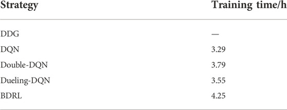
TABLE 4. Training time for offline and online strategies.

FIGURE 16

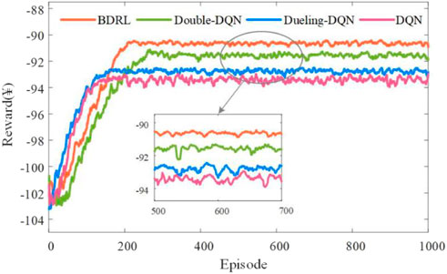
FIGURE 16. Comparison of rewards obtained by upper-level agents of DQN, Double-DQN, Dueling-DQN and BDDL methods.

FIGURE 17

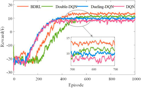
FIGURE 17. Comparison of rewards obtained by lower-level agents of DQN, Double-DQN, Dueling-DQN and BDDL methods.

From Table 4, DDG has no training process, because it does not contain the determination of neural network parameters. For the online strategies, the proposed BDRL method incorporates several extension improvement mechanisms and requires more neural network parameters to be determined. The training time of BDRL is 29.17% and 19.71% larger than that of Double-DQN and Dueling-DQN, respectively. Conversely, Dueling-DQN reduces the redundancy of the neural network structure, and its training time is less than that of Double-DQN. As depicted by Figures 16, 17, overall, the four algorithms achieve stable convergence from exploring the external environment to the final stable convergence. However, there are significant differences among the algorithms in terms of convergence speed, stability, and solution quality. Since our proposed method incorporates advanced extension improvement mechanisms from other methods, the learning rate can dynamically adjust according to training episodes. Besides, the interference of noise samples on the learning process can be eliminated, thus, the agents enter the stable convergence interval more quickly. Compared with other DQN methods, both upper-lower level agents for BDRL obtain the highest rewards, achieving ¥ -90.64 and ¥ 13.24, respectively. The basic DQN obtains faster convergence rates in both upper-lower levels, about 150 episodes and 350 episodes respectively. However, limited by the simple network structure and training mechanism, the basic DQN’s solution quality is relatively poor, and the final rewards are stable at ¥ -93.14 and ¥ 8.16, respectively. Further, the Double-DQN and Dueling-DQN algorithms improve respectively the neural network architecture as well as the Q-value computational paradigm. However, they need to be improved in terms of balancing the quality of exploration with the speed of exploitation. The cumulative average total cost of 100 days online testing for the above-mentioned offline and online strategies (namely, the cumulative of average daily time and cost of all owners) is shown in Figure 18.

FIGURE 18

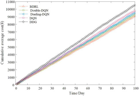
FIGURE 18. Cumulative average total cost of 100 days online testing for the offline and online strategies.

Besides, Figure 19 exhibits the average equilibrium degree of the charging service, and Table 5 lists the specific values of the traveling and charging evaluation indicators. Herein, all indicators in Table 5 are average values. Combining Figure 18 and Table 5, it can be seen that DDG, as a static guidance strategy, fails to adjust the decision output according to the real-time information variations. Thus, its cumulative average cost is the highest, reaching ¥ 10,518.36. Conversely, DQN, Double-DQN, Dueling-DQN and BDRL, as dynamic guidance strategies, have the capabilities of real-time environment perception and adaptive decision-making adjustment. Compared with DDG, their cumulative average costs are reduced by 7.06%, 11.60%, 9.47% and 13.75%, respectively.

FIGURE 19

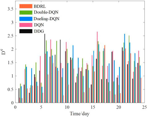
FIGURE 19. Average equilibrium degree of the charging service for offline and online strategies.

TABLE 5

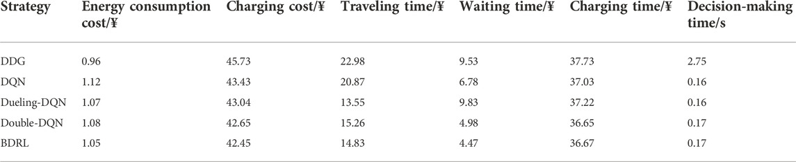
TABLE 5. Comparison of the traveling and charging evaluation indicators for offline and online strategies.

For the specific evaluation indicators, overall, charging costs account for the highest percentage of all five strategies, exceeding approximately 40%. It indicates that charging cost is the highest expense item for PEV owners. Clearly, DDG is a static guidance pattern based on the nearest CS recommendation and shortest path planning. Thus, the cost of each indicator is higher than that of DRL-based methods, except for the energy consumption cost. This means that the cost of energy consumption is proportional to the traveling distance. For decision-making time, there is no “offline training-online testing” paradigm in the DDG method, thus its decision-making time is larger than that of online decision-making methods. For DRL-based online decision-making methods, their decision-making time is controlled within seconds, meeting the real-time decision-making requirements of TECSs. Besides, the decision-making time of BDRL (0.17 s) is larger than that of DQN (0.16 s), which is caused by the retention of two decimal places after the decimal point and the calculation error of the server. The influence of the slight error on the decision-making time can be ignored. Moreover, our proposed BDRL method, based on the modified Rainbow architecture, enhances the ability of offline learning and online decision-making for discrete actions, and all indicators are higher than that of the DQN-based guidance strategies. The average equilibrium degree of the charging service for DQN, Double-DQN, Dueling-DQN and BDRL are 1.50, 1.51, 1.54 and 0.96, respectively. In summary, these results again demonstrate the superiority of BDRL in the case of charging and traveling decision-making support.

5 Conclusion

Based on the BDRL approach, this paper proposes a novel PEVDG. Clearly, the approach decouples the CS recommendation and path navigation tasks into an upper-lower level decision-making process. The actions and rewards in the upper-lower levels are specifically designed to improve the cooperation efficiency of dual agents. A modified Rainbow algorithm is proposed to enhance the learning ability and convergence performance. Case studies are performed within an urban TN with multiple CSs. The testing results show that the proposed method reduces the charging and traveling costs for PEV users and optimizes the node voltage distribution. By embedding the learning rate decay and the dropout layer technology, BDRL achieves promising decision-making performances, Compared with the offline guidance strategy (namely, DDG) and the DQN-based online guidance strategies (namely, DQN, Double-DQN, Dueling-DQN), the average cumulative rewards are reduced by 7.06%, 11.60%, 9.47% and 13.75%, respectively, and the average equilibrium degrees of the charging service are reduced by 27.81%, 36.00%, 36.42% and 37.66%, respectively. Besides, the average decision-making time for the DQN-based online guidance strategy is all within seconds, while that for the DDG-based strategy is about 3 s. One of the future directions is to evaluate the influencing factors of PEVDG, improving the scalability of the proposed model. Besides, the sensitivity analysis of network parameters for DRL will be further dissected.

Data availability statement

The raw data supporting the conclusion of this article will be made available by the authors, without undue reservation.

Author contributions

QX: Methodology, writing, and original draft preparation. ZC: Conceptualization and methodology. RS: Methodology, writing, and original draft preparation. ZZ: Review and editing.

Funding

This research was funded by the National Natural Science Foundation of China (52077035).

Acknowledgments

Thanks to the contributions of colleagues and institutions who assisted in this work.

Conflict of interest

The authors declare that the research was conducted in the absence of any commercial or financial relationships that could be construed as a potential conflict of interest.

Publisher’s note

All claims expressed in this article are solely those of the authors and do not necessarily represent those of their affiliated organizations, or those of the publisher, the editors and the reviewers. Any product that may be evaluated in this article, or claim that may be made by its manufacturer, is not guaranteed or endorsed by the publisher.

References

Alqahtani, M., and Hu, M. (2022). Dynamic energy scheduling and routing of multiple electric vehicles using deep reinforcement learning. Energy 244, 122626. doi:10.1016/j.energy.2021.122626

CrossRef Full Text | Google Scholar

Ding, T., Zeng, Z., Bai, J., Qin, B., Yang, Y., and Shahidehpour, M. (2020). Optimal electric vehicle charging strategy with Markov decision process and reinforcement learning technique. IEEE Trans. Ind. Appl. 56 (5), 5811–5823. doi:10.1109/tia.2020.2990096

CrossRef Full Text | Google Scholar

Duan, J., Shi, D., Diao, R., Li, H., Wang, Z., Zhang, B., et al. (2020). Deep-Reinforcement-Learning-Based autonomous voltage control for power grid operations. IEEE Trans. Power Syst. 35, 814–817. doi:10.1109/tpwrs.2019.2941134

CrossRef Full Text | Google Scholar

Hessel, M., Modayil, J., van Hasselt, H., Schaul, T., Ostrovski, G., and Dabney, W. et al (2017). Rainbow: Combining improvements in deep reinforcement learning.

Google Scholar

Hu, L., Dong, J., and Lin, Z. (2019). Modeling charging behavior of battery electric vehicle drivers: A cumulative prospect theory based approach. Transp. Res. Part C Emerg. Technol. 102, 474–489. doi:10.1016/j.trc.2019.03.027

CrossRef Full Text | Google Scholar

Ji, C., Liu, Y., Lyu, L., Li, X., Liu, C., Peng, Y., et al. (2020). A personalized Fast-Charging navigation strategy based on mutual effect of dynamic queuing. IEEE Trans. Ind. Appl. 56, 5729–5740. doi:10.1109/tia.2020.2985641

CrossRef Full Text | Google Scholar

Kancharla, S. R., and Ramadurai, G. (2020). Electric vehicle routing problem with non-linear charging and load-dependent discharging. Expert Syst. Appl. 160, 113714. doi:10.1016/j.eswa.2020.113714

CrossRef Full Text | Google Scholar

Lee, K., Ahmed, M. A., Kang, D., and Kim, Y. (2020). Deep reinforcement learning based optimal route and charging station selection. Energies 13, 6255. doi:10.3390/en13236255

CrossRef Full Text | Google Scholar

Li, X., Xiang, Y., Lyu, L., Ji, C., Zhang, Q., Teng, F., et al. (2020). Price Incentive-Based charging navigation strategy for electric vehicles. IEEE Trans. Ind. Appl. 56, 5762–5774. doi:10.1109/tia.2020.2981275

CrossRef Full Text | Google Scholar

Liu, C., Zhou, M., Wu, J., Long, C., and Wang, Y. (2019). Electric vehicles En-Route charging navigation systems: Joint charging and routing optimization. IEEE Trans. Control Syst. Technol. 27, 906–914. doi:10.1109/tcst.2017.2773520

CrossRef Full Text | Google Scholar

Lopez, K. L., Gagne, C., and Gardner, M. A. (2019). Demand-side management using deep learning for smart charging of electric vehicles. IEEE Trans. Smart Grid 10 (3), 2683–2691. doi:10.1109/tsg.2018.2808247

CrossRef Full Text | Google Scholar

Luo, L., Gu, W., Wu, Z., and Zhou, S. (2019). Joint planning of distributed generation and electric vehicle charging stations considering real-time charging navigation. Appl. Energy 242, 1274–1284. doi:10.1016/j.apenergy.2019.03.162

CrossRef Full Text | Google Scholar

Luo, Y., Feng, G., Wan, S., Zhang, S., Li, V., and Kong, W. (2020). Charging scheduling strategy for different electric vehicles with optimization for convenience of drivers, performance of transport system and distribution network. Energy 194, 116807. doi:10.1016/j.energy.2019.116807

CrossRef Full Text | Google Scholar

Morlock, F., Rolle, B., Bauer, M., and Sawodny, O. (2020). Time optimal routing of electric vehicles under consideration of available charging infrastructure and a detailed consumption model. IEEE Trans. Intell. Transp. Syst. 21, 5123–5135. doi:10.1109/tits.2019.2949053

CrossRef Full Text | Google Scholar

Qi, S., Lin, Z., Song, J., Lin, X., Liu, Y., Ni, M., et al. (2022). Research on charging-discharging operation strategy for electric vehicles based on different trip patterns for various city types in China. World Electr. Veh. J. 13, 7. doi:10.3390/wevj13010007

CrossRef Full Text | Google Scholar

Qian, T., Shao, C., Li, X., Wang, X., and Shahidehpour, M. (2020b). Enhanced coordinated operations of electric power and transportation networks via EV charging services. IEEE Trans. Smart Grid 11 (4), 3019–3030. doi:10.1109/TSG.2020.2969650

CrossRef Full Text | Google Scholar

Qian, T., Shao, C., Wang, X., and Shahidehpour, M. (2020a). Deep reinforcement learning for EV charging navigation by coordinating smart grid and intelligent transportation system. IEEE Trans. Smart Grid 11, 1714–1723. doi:10.1109/tsg.2019.2942593

CrossRef Full Text | Google Scholar

Shi, X., Xu, Y., Guo, Q., Sun, H., and Gu, W. (2020). A distributed EV navigation strategy considering the interaction between power system and traffic network. IEEE Trans. Smart Grid 11 (4), 3545–3557. doi:10.1109/tsg.2020.2965568

CrossRef Full Text | Google Scholar

Sohet, B., Hayel, Y., Beaude, O., and Jeandin, A. (2021). Hierarchical coupled driving-and-charging model of electric vehicles, stations and grid operators. IEEE Trans. Smart Grid 12 (6), 5146–5157. doi:10.1109/tsg.2021.3107896

CrossRef Full Text | Google Scholar

Srivastava, N., Hinton, G., Krizhevsky, A., Sutskever, I., and Salakhutdinov, R. (2014). Dropout: A simple way to prevent neural networks from overfitting. J. Mach. Learn. Res. 15, 1929–1958.

Google Scholar

Sun, G., Li, G., Xia, S., Shahidehpour, M., Lu, X., and Chan, K. W. (2020). ALADIN-based coordinated operation of power distribution and traffic networks with electric vehicles. IEEE Trans. Ind. Appl. 56 (5), 5944–5954. doi:10.1109/tia.2020.2990887

CrossRef Full Text | Google Scholar

Tu, Q., Cheng, L., Yuan, T., Cheng, Y., and Li, M. (2020). The constrained reliable shortest path problem for electric vehicles in the urban transportation network. J. Clean. Prod. 261, 121130. doi:10.1016/j.jclepro.2020.121130

CrossRef Full Text | Google Scholar

Wang, E., Ding, R., Yang, Z., Jin, H., Miao, C., Su, L., et al. (2022). Joint charging and relocation recommendation for E-taxi drivers via multi-agent mean field hierarchical reinforcement learning. IEEE Trans. Mob. Comput. 21 (4), 1274–1290. doi:10.1109/tmc.2020.3022173

CrossRef Full Text | Google Scholar

Wang, J., Elbery, A., and Rakha, H. A. (2019). A real-time vehicle-specific eco-routing model for on-board navigation applications capturing transient vehicle behavior. Transp. Res. Part C Emerg. Technol. 104, 1–21. doi:10.1016/j.trc.2019.04.017

CrossRef Full Text | Google Scholar

Wang, Y., Bi, J., Zhao, X., and Guan, W. (2018). A geometry-based algorithm to provide guidance for electric vehicle charging. Transp. Res. Part D Transp. Environ. 63, 890–906. doi:10.1016/j.trd.2018.07.017

CrossRef Full Text | Google Scholar

Xiang, Y., Yang, J., Li, X., Gu, C., and Zhang, S. (2022). Routing optimization of electric vehicles for charging with Event-Driven pricing strategy. IEEE Trans. Autom. Sci. Eng. 19, 7–20. doi:10.1109/tase.2021.3102997

CrossRef Full Text | Google Scholar

Xing, Q., Chen, Z., Zhang, Z., Huang, X., and Li, X. (2020). Route planning and charging navigation strategy for electric vehicles based on real-time traffic information and Grid Information. IOP Conf. Ser. Mat. Sci. Eng. 752 (1). 012011. doi:10.1088/1757-899X

CrossRef Full Text | Google Scholar

Yu, J. J. Q., Yu, W., and Gu, J. (2019). Online vehicle routing with neural combinatorial optimization and deep reinforcement learning. IEEE Trans. Intell. Transp. Syst. 20, 3806–3817. doi:10.1109/tits.2019.2909109

CrossRef Full Text | Google Scholar

Zhang, C., Liu, Y., Wu, F., Tang, B., and Fan, W. (2021). Effective charging planning based on deep reinforcement learning for electric vehicles. IEEE Trans. Intell. Transp. Syst. 22, 542–554. doi:10.1109/tits.2020.3002271

CrossRef Full Text | Google Scholar

Zhang, W., Liu, H., Xiong, H., Xu, T., Wang, F., Xin, H., et al. (2022). RLCharge: Imitative multi-agent spatiotemporal reinforcement learning for electric vehicle charging station recommendation. IEEE Trans. Knowl. Data Eng. 4347 (3), 1–14. doi:10.1109/tkde.2022.3178819

CrossRef Full Text | Google Scholar

Zhang, Y., Wang, X., Wang, J., and Zhang, Y. (2021). Deep reinforcement learning based Volt-VAR optimization in smart distribution systems. IEEE Trans. Smart Grid 12, 361–371. doi:10.1109/tsg.2020.3010130

CrossRef Full Text | Google Scholar

Zhao, J., Mao, M., Zhao, X., and Zou, J. (2021). A hybrid of deep reinforcement learning and local search for the vehicle routing problems. IEEE Trans. Intell. Transp. Syst. 22, 7208–7218. doi:10.1109/tits.2020.3003163

CrossRef Full Text | Google Scholar

Zhou, Y., Yuan, Q., Tang, Y., Wu, X., and Zhou, L. (2021). Charging decision optimization for electric vehicles based on traffic-grid coupling networks. Power Syst. Technol. 45, 3563–3572.

Google Scholar

Zou, Y., Wei, S., Sun, F., Hu, X., and Shiao, Y. (2016). Large-scale deployment of electric taxis in beijing: A real-world analysis. Energy 100, 25–39. doi:10.1016/j.energy.2016.01.062

CrossRef Full Text | Google Scholar