Wind power probabilistic forecasting based on combined decomposition and deep learning quantile regression

1 Introduction

The limitation of fossil fuels and the environmental degradation caused by fossil fuels have restricted the increasing global demand for electricity. Countries around the world are promoting the rapid development of clean energy represented by wind energy. In 2021, the newly installed wind power capacity in the world exceeded 94 GW (Global Wind Energy Council (GWEC), 2022). Due to the randomness, volatility and intermittent of wind power, the large-scale grid connection of wind power brings great uncertainty and risks to the supply side of the power system (Georgilakis, 2008). Therefore, accurate and reliable wind power forecasting is important to the safe operation of the power system and the utilization of wind energy (Jin et al., 2021).

Wind power prediction methods are mainly divided into deterministic prediction and probabilistic prediction (Zhou et al., 2021). Deterministic prediction is achieved through point prediction models which have three types: statistical models, machine learning models, and deep learning models. Many statistical models have been applied to wind power prediction, such as kalman filter (KF) (Liu and Liang, 2021), auto regressive moving average (ARMA) (Erdem and Shi, 2011), auto regressive integrated average (ARIMA) (Amini et al., 2016), etc. Commonly used machine learning models include artificial neural network (ANN) (Ren et al., 2014), support vector machine (SVM) (Demolli et al., 2019), etc.

Compared with statistical and machine learning models, deep learning models have stronger nonlinear mapping capabilities. With the development of deep learning technology, some deep neural network (DNN) models have been applied to renewable energy prediction, including deep belif network (DBN) (Wang et al., 2018), convolutional neural network (CNN) (Oh et al., 2019; Hong and Satriani, 2020; Huang et al., 2022), recurrent neural network (RNN) (Yu et al., 2018) etc. Ordinary RNN models suffering from the gradient vanishment and gradient explosion are rarely used to predict wind power (Zang et al., 2021), while its variants long short term memory neural network (LSTM) (Yuan et al., 2019; Wang et al., 2020; Zang et al., 2021) and gated recurrent unit (GRU) (Niu et al., 2020; Peng et al., 2020; Kisvari et al., 2021) can deal with the long-term dependency through specific internal structures.

The models mentioned above are all point prediction models. The expected values of wind power are obtained while the results are incapable of quantifying the uncertainty. Especially when the wind power fluctuates strongly, the point prediction may be less reliable and cannot meet the actual scheduling requirements. Therefore, the probability density and interval prediction of wind power have more significance in practical application and become a hot research direction recently (Wang et al., 2017; Zhang et al., 2019; Zhou et al., 2021).

Wind power probabilistic prediction can provide the probability density functions of wind power at the future time or the fluctuation interval under a certain degree of confidence (Zhang et al., 2016). Commonly used probabilistic prediction methods include error analysis method (Lv et al., 2021), upper and lower bound estimation method (Liu et al., 2020), quantile regression method (QR) (He and Li, 2018), etc. QR can construct the relationship between the input and the output of different quantiles, combined with the kernel density estimation (KDE) can achieve probabilistic prediction. QR is essentially a linear model, and its ability to express nonlinear data is poor. Some variants of QR models such as neural network QR solve this problem by combining QR with BP neural network (He and Li, 2018). In Ref. (Zhang et al., 2019), a framework combining the point prediction model with QR was proposed to achieve probabilistic prediction. QRLSTM, QRGRU and QRMGM were proposed to prove the effectiveness of the proposed framework. In Ref. (Peng et al., 2021), a model called EALSTM-QR was designed, which combined QR, LSTM, Encoder and Attention to improve the non-linear expression of data. Yao et al. (He and Wang, 2021) combined the LASSO regression with the QRNN model, and used ensemble empirical mode decomposition (EEMD) to reduce the complexity of the wind power sequence, which effectively improved the prediction accuracy. In Ref. (Sun et al., 2022), a quantile regression forest interval prediction model is proposed for multiple fluctuation processes for ultra-short-term time scales.

Many scholars have proposed hybrid models that combine data decomposition technology and prediction model to further improve the accuracy of wind power prediction (Zhang et al., 2021). Common data decomposition methods include empirical mode decomposition (Bokde et al., 2018) (EMD), EEMD (Santhosh et al., 2018), empirical wavelet transform (Hu and Wang, 2015) (EWT), variational mode decomposition (Dragomiretskiy and Zosso, 2014) (VMD), singular spectrum analysis (Yu et al., 2017a) (SSA), etc. In Ref. (Han et al., 2019), a prediction method combining VMD and LSTM (VMD-LSTM) is proposed to improve the accuracy of multi-step wind power prediction. Similar to other combined models, VMD is used to decompose wind power data into trend, periods and random components; then, LSTM is used to deeply learn the characteristics of the three components. Some studies combine different decomposition methods to improve the overall prediction performance. Sun et al. (Sun et al., 2021) proposes a secondary decomposition strategy, which combines EWT and VMD to comprehensively filter out the instability and noise of the wind power sequence. In Ref. (Yu et al., 2017b), a hybrid model that combines EMD, SSA and Elman uses SSA to reprocess the highest-frequency component of the EMD component to improve the accuracy of prediction.

Data of numerical weather prediction (NWP) includes forecast data such as wind speed, wind direction, humidity, etc., which including features related to wind power (Wu et al., 2021). Using NWP data as a feature input can improve the prediction performance of wind power (Wang et al., 2021). The information contained in NWP data is complex and diverse. Effective methods need to be used to extract the dynamic features of NWP data as input to the predictive model. Hao et al. (Yin et al., 2021) designed a feature extractor called CNNs-LSTM, which uses CNN and LSTM to extract meteorological and temporal features of wind farms. Zang et al. (Zang et al., 2020b) proposed a CNN-LSTM model, which applies CNN to extract spatial features from meteorological data, and LSTM extracts temporal features from historical solar irradiance time series data. In (Cheng et al., 2022), a model based on CNN and LSTM is proposed for prediction of satellite-derived solar irradiance and improves its learning ability relative to traditional learning models. In Ref. (Wang et al., 2022), a load probability density forecasting model based on convolutional long short-term memory (ConvLSTM) is proposed to capture the deep information. CNN has powerful capabilities of feature extraction and non-linear expression, which can effectively extract important information from input data (Zang et al., 2020a). GRU has powerful capabilities of time series analysis and learning, and can effectively extract the time series features of the sequence. This study uses the feature extraction module that combines CNN and Bi-directional GRU (BGRU) to extract features from NWP data.

There are many studies based on wind power point forecasting, but there is a lack of wind power probability forecasting models that combine the advantages of combinatorial decomposition techniques and deep neural networks. Reliable probabilistic predictions and accurate point predictions of wind power need to be achieved simultaneously. Based on the above analysis, this study proposes a novel wind power probabilistic prediction model combining VMD, SSA, QR, CNN, and BGRU (VMDS-QR-CBG). First, wind power history sequence is processed by VMDS, where the SSA improves VMD though making further operation on the high-frequency components of the VMD. Next, the BGRU extracts the timing features of the low-frequency components of the wind power; CBG is used to extract the complex dynamic features of high-frequency components and NWP data respectively. Then, BGRU further extracts deep time-series features of all the extracted features, and establishes a QR model to obtain predicted values at different quantile conditions. Finally, the probability density function curve (PDF) of wind power is obtained by kernel density estimation (KDE) to achieve probabilistic prediction. The model can also achieve reliable point and interval prediction. According to the discussions above, the main contributions of this study can be summarized as follows:

• A novel combined data decomposition method called VMDS is proposed, which combines VMD and SSA to reduce the complexity of the original wind power sequence and further extract the high-frequency trend components. The input data processed by VMDS helps to improve the accuracy of the prediction model.

• A feature extractor called CBG that combines CNN and BGRU is used to extract features from complex data, including meteorological data and high-frequency data.

• A hybrid VMDS-QR-CBG model with three input channels is developed by combining VMDS and CBG and QR to achieve reliable wind power point and probabilistic prediction.

2 Proposed methodology

2.1 General process of the proposed method

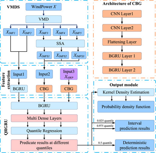
This section introduces the proposed model of wind power probabilistic prediction. The flow chart of VMDS-QR-CBG is shown in Figure 1, where the forecasting process can be summarized as follows:

• VMDS for data decomposition.

FIGURE 1

FIGURE 1. Structure diagram of VMDS-QRCNN-BGRU.

The wind power sequence is decomposed into several components using the proposed data decomposition method VMDS. The low-frequency components and high-frequency trend components are used as inputs to different channels.

• Feature extraction.

The input of the proposed model has three kinds of data, namely VMD components X_IMF, SSA components X_IMFS and NWP data X_NWP. The features of the data are extracted by different modules. The features extracted by each module are combined into X_f, which is used as the input of subsequent modules.

• Probabilistic forecasting.

A probability prediction module based on QR and BGRU is constructed, and prediction values under different quantiles are obtained according to fusion features X_f. At the same time, deterministic forecast results and interval forecast results are obtained. KDE is used to obtain the PDF curve of the predicted value.

2.2 Combination decomposition VMDS

VMDS is a combined decomposition method composed of VMD and SSA. Considering the degree of data utilization and the training cost of the model, VMDS is used to decompose the wind power data into 5 components. The main process is:

• VMD is used to decompose the wind power sequence X into sub-sequences, X_IMF1 to X_IMF5, where X_IMF1, and X_IMF2 are low-frequency components, X_IMF3 to X_IMF5 are high frequency-components.

• SSA is used to extract trend components of X_IMF3 to X_IMF5 to reduce the complexity of the sequence and highlight the timing feature of the sequence. The trend components are defined as X_IMFS1, X_IMFS2, and X_IMFS3.

The principles of VMD and SSA are as follows.

2.2.1 Variational mode decomposition

VMD technology is a non-recursive signal multi-resolution decomposition technology, which can decompose a complex signal S into q modal functions with different center frequencies (Hu and Wang, 2015). The specific steps of VMD are as follows:

Calculate the unilateral frequency spectrum of each mode based on the Hilbert transform method. Perform exponential correction for each modal component to shift its phase to the center frequency of the modal itself.

According to the Gaussian smoothness of the frequency-shifted signal, the bandwidth is estimated to minimize the sum of the estimated bandwidth of each sub-signal.

$\begin{array}{l}\underset{u_k,{\omega }_k}{\min }\left\{{\displaystyle \sum _k{\Vert \partial t\left[\left(\delta \left(t\right)+\frac{j}{\pi t}\right)\text{∗}{u}_k\left(t\right)\right]e^{-j{\omega }_{k}t}\Vert }_2}\right\}\\ s.t.S\left(t\right)={\displaystyle \sum _k{u}_k\left(t\right)}\end{array}(1)$

The augmented Lagrangian function is introduced to turn the constrained variational problem into an unconstrained problem:

$\begin{array}{l}L\left(u_k,{\omega }_k,\lambda \right)=\beta {\displaystyle \sum _k\left|\right|\partial t\left[\left(\delta \left(t\right)+\frac{j}{\pi t}\right)\text{∗}{u}_k\left(t\right)\right]e^{-j{\omega }_{k}t}|{|}_2}\\ +\left|\right|S\left(t\right)-{\displaystyle \sum _k{u}_k\left(t\right)}{\text{||}}_2+<\lambda \left(t\right),S\left(t\right)-{\displaystyle \sum _k{u}_k\left(t\right)}>\end{array}(2)$

Solve the Eq. 2 by the alternating direction multiplier method, obtain the required q modal components $u_k$, and the center frequency ${\omega }_k$.

2.2.2 Singular spectrum analysis

SSA constructs a trajectory matrix based on the observed time series, and decomposes and reconstructs the trajectory matrix, thereby extracting sub-sequences representing different components of the original time series (Dragomiretskiy and Zosso, 2014). The specific steps of SSA are as follows:

Select the appropriate embedding dimension L to transform the time series X_n = (x₁, ..., x_n) into the trajectory matrix A.

$A=\left(\begin{array}{ccccc}{x}_1& x_2& x_3& \cdots & x_{M-L+1}\\ x_2& x_3& x_4& \cdots & x_{M-L+2}\\ ⋮& ⋮& ⋮& \cdots & ⋮\\ x_L& x_{L+1}& x_{L+2}& \cdots & x_M\end{array}\right)(3)$

Perform singular value decomposition (SVD) on matrix A, and the SVD formula is as follows:

$A={\displaystyle \sum _{i=1}^{rank\left(X\right)}\sqrt{{\lambda }_i}{U}_i{V}_i^T}(4)$

Use the diagonal averaging method to transform the decomposition matrix A into a matrix of length M. The formula for diagonal averaging is as follows:

$x_k^{\ast }=\{\begin{array}{l}\begin{array}{cc}\frac{1}{k}{\displaystyle \sum _{m=1}^k{x}_{m,k-m+1}^{\ast }}& 1\le k<L^{\ast }\end{array}\\ \begin{array}{cc}\frac{1}{L^{\ast }}{\displaystyle \sum _{m=1}^{L^{\ast }}{x}_{m,k-m+1}^{\ast }}& L^{\ast }\le k<Q^{\ast }\end{array}\\ \begin{array}{cc}\frac{1}{M-k+1}{\displaystyle \sum _{m=k-Q^{\ast }+1}^{M-k+1}{x}_{m,k-m+1}^{\ast }}& Q^{\ast }\le k<M\end{array}\end{array}(5)$

Where the number of vectors $Q=M-L+1$, $L^{\ast }=\min \left(L,Q\right)$, $Q^{\ast }=\max \left(L,Q\right)$.

2.3 Feature extraction based on deep neural network

The DNNs mainly used in the model are CNN and BGRU. Construct different feature extraction modules for different inputs:

• The feature extraction of X_IMF mainly considers the trend component X_IMF1 and the periodic component X_IMF2. Their fluctuation frequency is low and the trend is obvious. Therefore, a two-layer BGRU is used to extract the features of X_IMF.

• The fluctuation frequency of X_IMFS is high and the trend is not obvious. Therefore, the feature extraction module that combines CNN and BGRU (CBG) is used to extract the complex dynamic features of X_IMFS. The structure of CBG is cascaded, mainly including two layers of CNN and two layers of BGRU.

• X_NWP contains many non-linear and low-correlation factors. The CBG module is used to extract the spatiotemporal features of the impact of X_NWP on wind power.

The principles of CNN and BGRU are as follows.

2.3.1 Convolutional neural network

CNN is a DNN with pooling operation, local connection, and weight sharing based on convolution operation. It is widely used to extract high-order features from complex data. 1D-CNN structure mainly includes convolutional layer, pooling layer, and fully connected layer (Huang et al., 2022).

The function of the convolutional layer is to extract features from the input data by scanning through the convolution kernel. The convolution formula is shown in Eq. 6. The function of the pooling layer is to extract the convolutional layer. The features of the feature vector are sampled, and while retaining the main information of the feature vector, it can reduce the dimension of the feature vector and the complexity of the network. The fully connected layer is mainly used to integrate the features extracted by the network, and then output the final feature vector of a specific dimension after processing methods such as activation functions. The overall calculation formula is shown in Eq. 7.

$y_p^l=r\left({\displaystyle \sum _{q\in T_{l-1}}{x}_q^{l-1}}\ast v_p^l+b_p^l\right),p\in T_l(6)$

$y_j^l=\sigma \left({\displaystyle \sum _{i=1}^{N_{l-1}}{W}_{ij}{x}_i^{l-1}+b_j^l}\right)(7)$

2.3.2 Bi-directional gated recurrent unit

GRU optimizes and improves LSTM, reduces network complexity, and maintains a learning performance equivalent to LSTM (Peng et al., 2020). The gated loop unit in GRU has two gate structures: an update gate and a reset gate. The update gate controls the degree of retention of the state at the previous moment in the current state, and the reset gate controls the degree of combination of the current input and the state at the previous moment. The calculation formula of the hidden layer state $h_t$ of GRU is as follows:

$z_t=\sigma \left(W_{zx}{x}_t+W_{zh}{h}_{t-1}+b_z\right)(8)$

$r_t=\sigma \left(W_{rx}{x}_t+W_{rh}{h}_{t-1}+b_r\right)(9)$

${\tilde{h}}_t=\tanh \left(W_{\tilde{h}h}\left(r_t\odot h_{t-1}\right)+W_{\tilde{h}x}{x}_t+b_{\tilde{h}}\right)(10)$

$h_t=\left(1-z_t\right)\odot h_{t-1}+z_t\odot {\tilde{h}}_t(11)$

GRU can make full use of the information of the current and previous moments, but cannot obtain the unit information after the current moment. BGRU combines two GRU networks with opposite timings to fully obtain the hidden information before and after the current unit, and further mine timing features.

2.4 Probabilistic prediction module

According to the fusion features obtained by the feature extraction module, a prediction model based on BGRU and QR is constructed.

Use BGRU to extract deeper timing features of X_f, and send the results to the multi dense layers for processing. The process can be expressed as:

$y=f\left(W,b,X_{in}\right)(12)$

Construct the quantile loss function as in Eq. 13 to realize quantile regression.

$\tilde{W}\left(\tau \right),\tilde{b}\left(\tau \right)=\underset{W,b}{\arg \min }{\displaystyle \sum _{t=1}^n{\rho }_{\tau }\left(y_t-f\left(W\left(\tau \right),b\left(\tau \right),X_t\right)\right)}(13)$

${\rho }_{\tau }\left(\mu \right)=\mu \left(\tau -I\left(\mu \right)\right),I\left(\mu \right)=\{\begin{array}{l}1,\mu <0\\ 0,\mu \ge 0\end{array}(14)$

Where the quantile τ is continuously taken in the range of (0,1), the Adam gradient descent algorithm is used to optimize Eq. 13 to obtain the optimal estimated values of network parameters W(τ) and b(τ) under different quantile conditions. Furthermore, the predicted value of wind power at different quantile conditions can be obtained according to Eq. 14.

$\tilde{y}\left(\tau \right)=f\left(\tilde{W}\left(\tau \right),\tilde{b}\left(\tau \right),X_{in}\right)(15)$

After obtaining the predicted values at different quantiles, the deterministic prediction results and interval prediction results can be obtained, which are $\tilde{y}\left(\text{0}\text{.}5\right)$ and $\left[\tilde{y}\left({\tau }_{down}\right),\tilde{y}\left({\tau }_{up}\right)\right]$ respectively. ${\tau }_{down}$ and ${\tau }_{up}$ are determined by the confidence of the prediction interval. ${\tau }_{down}=\text{0}\text{.}5\alpha$ and ${\tau }_{up}=\text{1}-\text{0}\text{.}5\alpha$ while the prediction interval confidence is $1-\alpha$.

KDE is a classic non-parametric estimation method that does not require prior assumptions (Zhang et al., 2019). Provided at a given point y, the prediction value of the prediction model at each quantile is $\widehat{y}$ = [${\widehat{y}}_1$, ${\widehat{y}}_2$,…, ${\widehat{y}}_N$], the probability density function of y at a formula:

$P\left(y\right)=\frac{1}{nB}{\displaystyle \sum _{i=1}^{n}K\left(\frac{y_i-y}{B}\right)}(16)$

Where B is the bandwidth, using grid search with cross-validation to select the appropriate bandwidth. This study uses the Epanechnikov as kernel function, the formula is as follows:

$K\left(\mu \right)=\{\begin{array}{cc}\frac{3}{4}\left(1-{\mu }^2\right),& \mu \in \left[-\mathrm{1,1}\right]\\ 0,& \mu \notin \left[-\mathrm{1,1}\right]\end{array}(17)$

KDE is used to fit the predicted values at different quantiles to obtain the final PDF to achieve probability density prediction.

3 Performance indicators

3.1 Evaluation metrics of deterministic prediction

This study uses root mean square error (RMSE) and normalized mean absolute percentage error (NMAPE) to evaluate the deterministic prediction performance of the prediction model (Zhang et al., 2019). The formulas are as follow:

$RMSE=\sqrt{\frac{1}{n}{\displaystyle \sum _{i=1}^n{\left(y_i-{\widehat{y}}_i\right)}^2}}(18)$

$NMAPE=\frac{1}{n}{\displaystyle \sum _{i=1}^n\frac{|y_i-{\widehat{y}}_i|}{\underset{i=1}{\overset{n}{\max }}{y}_i}}\times 100\%(19)$

The smaller the RMSE and NMAPE values, the better the performance of the deterministic prediction model.

3.2 Evaluation metrics of interval prediction

This study uses average coverage error (ACE), prediction interval normalized average width (PINAW), and interval sharpness (IS) to evaluate interval prediction performance (Zhang et al., 2019). The formula is as follows:

$ACE=\left(\frac{1}{n}{\displaystyle \sum _{i=1}^n\{\begin{array}{l}1,y_i\in \left[l_i^{\alpha },u_i^{\alpha }\right]\\ 0,y_i\notin \left[l_i^{\alpha },u_i^{\alpha }\right]\end{array}}-\left(1-\alpha \right)\right)\times 100\%(20)$

$PINAW=\frac{1}{ns}{\displaystyle \sum _{i=1}^n\left(u_i^{\alpha }-l_i^{\alpha }\right)}(21)$

$IS=\frac{1}{n}{\displaystyle \sum _{i=1}^n\{\begin{array}{l}-2\alpha \left(u_i^{\alpha }-l_i^{\alpha }\right),y_i\in \left[l_i^{\alpha },u_i^{\alpha }\right]\\ -2\alpha \left(u_i^{\alpha }-l_i^{\alpha }\right)-4\left(l_i^{\alpha }-y_i\right),y_i<l_i^{\alpha }\\ -2\alpha \left(u_i^{\alpha }-l_i^{\alpha }\right)-4\left(y_i-u_i^{\alpha }\right),y_i>u_i^{\alpha }\end{array}}(22)$

ACE represents the coverage of the actual value in the prediction area under a given confidence interval, and reflects the reliability of the interval prediction. PINAW is used to measure the width of the prediction interval and reflects the acuity of interval prediction. IS measures the comprehensive performance of interval prediction, because ACE and PINAW are a pair of contradictory indicators.

3.3 Evaluation metrics of probabilistic prediction

This study uses continuous ranked probability score (CRPS) to evaluate probabilistic prediction performance (Peng et al., 2021). The formula is as follows:

$CRPS=\frac{1}{n}{\displaystyle \sum _{i=1}^n{\displaystyle \underset{-\infty }{\overset{+\infty }{\int }}{\left[F\left(y_i\right)-I\left({\widehat{y}}_i-y_i\right)\right]}^2\text{d}{y}_i}}(23)$

$F\left(y_i\right)={\displaystyle {\int }_{-\infty }^{y_i}P\left(x_i\right)d{x}_i}(24)$

The smaller the CRPS, the better the overall performance of the model’s probabilistic prediction and the higher the reliability.

4 Testing results and discussions

4.1 Datasets

The original data comes from a wind farm in Jiangsu, China, which contains the wind power series data and NWP data for the whole year of 2017. Wind power data is collected every 15 min, so there are 96 data points in a day. Table 1 shows the basic information of the data set. The dataset has strong nonlinearity and non-stationarity. NWP data includes wind speed at different heights, wind direction at different heights, temperature, air pressure, humidity, etc.

TABLE 1

TABLE 1. The basic information of data set.

In the experiment of this study, the input dimensions of wind power data and NWP data are both set to 10. The first 80% of each data set is used as the training set, and the last 20% is used as the test set.

4.2 Result of VMDS

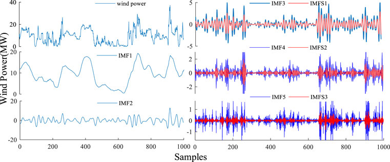
The wind power sequence is processed by VMDS to obtain two low-frequency components and three high-frequency components. The partial decomposition result of Dataset is shown in Figure 2, where IMF1 to IMF5 are the results of VMD, and IMFS1 to IMFS3 are the results of further processing by SSA. VMD parameters are set as: penalty parameter is 1,000; initial center frequency is 0; convergence criterion is 10^–6. SSA parameters are set as: Embedded window length is 10.

FIGURE 2

FIGURE 2. Original wind power and VMDS decomposition results.

4.3 Models and parameter settings

Several predictive models were proposed as comparison models to verify the superiority of the comprehensive predictive performance of VMDS-QR-CBG. The models are VMD-QR-CBG, VMDS-QRGRU, QRCNN-GRU, QRLSTM, QRGRU. VMD-QR-CBG is used to illustrate the superiority of VMDS. VMDS-QRGRU is used to reflect the effect of proposed module of multi-source feature extraction. QRCNN-GRU, QRLSTM, QRGRU are common deep learning models that do not use data decomposition technology, which reflect the overall performance of the proposed combined model.

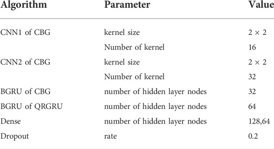
The main layer design and hyperparameter settings of VMDS-QR-CBG are shown in Table 2. The setting of the model parameters is obtained through multiple experiments and is suitable for the scale of the dataset. The settings of the hyperparameters of the comparison models are kept as uniform as possible to reflect the superiority of the proposed combined model under a unified hyperparameter setting. The training configuration of the five models is the same: the training round is 200, the optimizer is Adam, the early stop waiting round is 10, and the validation set ratio is 0.1. The model proposed in this study sets 199 quantile points, and quantile points $\tau$ = [0.005, 0.01, ..., 0.99, 0.995].

TABLE 2

TABLE 2. The main parameter settings of VMDS-QR-CBG.

4.4 Analysis of prediction result

4.4.1 Probability density prediction results

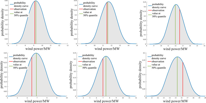
The predicted value at different quantiles obtained by the models using QR, can estimate the PDF of each observation point through KDE. Figure 3 shows the PDFs of six randomly selected observation points for the dataset. Figure 3 shows that most of the actual values are close to the peak of the PDF and close to the predicted median. This shows that the proposed probabilistic prediction model is effective.

FIGURE 3

FIGURE 3. PDF at different moments predicted by VMDS-QR-CBG.

Table 3 shows the value of the CRPS of the probabilistic prediction results of different models. Among them, the CRPS of VMDS-QR-CBG is the smallest, indicating that the comprehensive performance of the probabilistic prediction of VMDS-QR-CBG is the highest.

TABLE 3

TABLE 3. The values of the CRPS of different models.

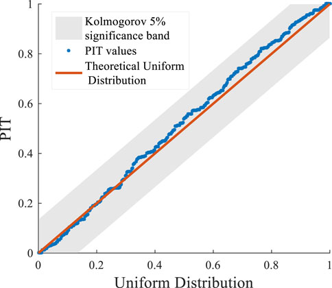
By calculating the probability integral transformation (PIT) of the predicted value and analyzing whether it obeys a uniform distribution, the reliability of the probabilistic prediction model can be verified. The QQ chart is used to visually analyze whether the PIT value of the prediction model result obeys a uniform distribution.

Figure 4 is the QQ plot of the PIT values of the probabilistic prediction results of VMDS-QR-CBG. The red straight line is the uniform distribution of the theoretical situation, and the blue is the probability distribution of the predicted value of the PIT value. It can be seen from Figure 4 that the distribution of the PIT values are in the Kolmogorov 5% significant band, which shows that the probabilistic prediction results of VMDS-QR-CBG are reliable.

FIGURE 4

FIGURE 4. QQ plot of probability prediction results of VMDS-QR-CBG.

4.4.2 Analysis of interval prediction results

Excellent interval prediction performance requires that the acuity of prediction should be improved as much as possible while ensuring the reliability of prediction. Table 4 shows the error statistics of the interval prediction of each model, including evaluation indicators: PINAW, ACE, IS. The following conclusions can be drawn: Compared with models using data decomposition technology, the evaluation indicators of QRCNN-GRU, QRLSTM, QRGRU models are much inferior. The ACE value of the models without the decomposition technology is generally higher than that of the model using the decomposition technology. However, the PINAW value is much lower than the model using decomposition technology. This shows that the prediction interval of models such as QRCNN-GRU is relatively wide, so that the reliability of prediction is improved, but the acuity of prediction is reduced, thereby reducing the overall performance of interval prediction. The IS values of the model using VMD or VMDS are 0.1–0.5 lower than the IS value of models such as QRCNN-GRU. In summary, compared to traditional models that do not use data decomposition technology, the interval prediction of VMDS-QR-CBG has better performance.

TABLE 4

TABLE 4. Interval predication error statistics of different models.

The comparison of the interval prediction performance of VMDS-QR-CBG and VMD-QR-CBG is to verify the effectiveness of the proposed VMDS. The ACE value of VMDS-QR-CBG is lower than that of VMD-QR-CBG, which shows that the reliability of VMD-QR-CBG is slightly higher than that of VMDS-QR-CBG. However, the PINAW value of VMDS-QR-CBG is respectively lower than VMD-QR-CBG by 14.9%. The IS value of VMDS-QR-CBG is respectively higher than VMD-QR-CBG by 18.8%. The above analysis shows that the proposed VMDS method is helpful to the improvement of the model’s interval prediction performance.

The comparison between the interval prediction performance of VMDS-QR-CBG and VMDS-QR-GRU is to verify the effectiveness of the proposed combined model. The PINAW value of VMDS-QR-CBG is respectively lower than VMDS-QR-GRU by 20.3%. Moreover, the IS value of VMDS-QR-CBG is respectively higher than VMDS-QR-GRU by 14.4%. The above analysis can show that the proposed combination method using CBG to extract the dynamic features of the NWP data and SSA components is effective.

The interval prediction results are shown in Figure 5. All models have good prediction performance, but the interval width of VMDS-QR-CBG is significantly narrower than that of other models. VMDS-QR-CBG can both ensure reliability and high sensitivity in wind power with large fluctuations.

FIGURE 5

FIGURE 5. Interval prediction results of Datast1 of different models.

4.4.3 Analysis of deterministic prediction results

This study selects the median of the probabilistic prediction results of each model as the deterministic prediction result of wind power.

Table 5 shows that the RMSE and NMAPE of VMDS-QR-CBG are the lowest. RMSE decreased by 13.6, 8.6, 16.2, 31.5 and 32.2% respectively compared with other models. NMAPE decreased by 0.300, 0.176, 0.312, 0.699 and 0.773 respectively compared with other models.

TABLE 5

TABLE 5. Deterministic predication error statistics of different models.

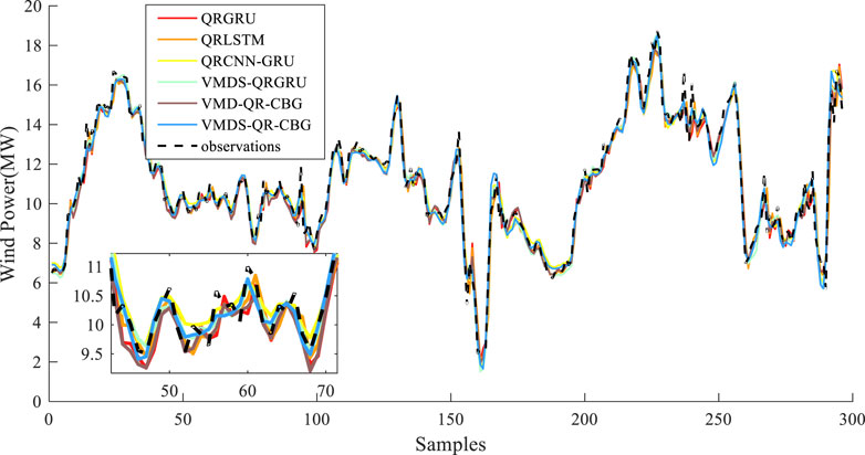
Figure 6 is a comparison diagram between the predicted values of each model and the actual value of wind power. Figure 6 shows that each model can accurately predict the change trend of wind power, and the predicted value of the VMDS-QR-CBG model is the closest to the actual value of wind power. In summary, VMDS-QR-CBG can better ensure accurate deterministic prediction of wind power.

FIGURE 6

FIGURE 6. Point prediction results of Datast1 of different models.

4.4.4 Generality verification

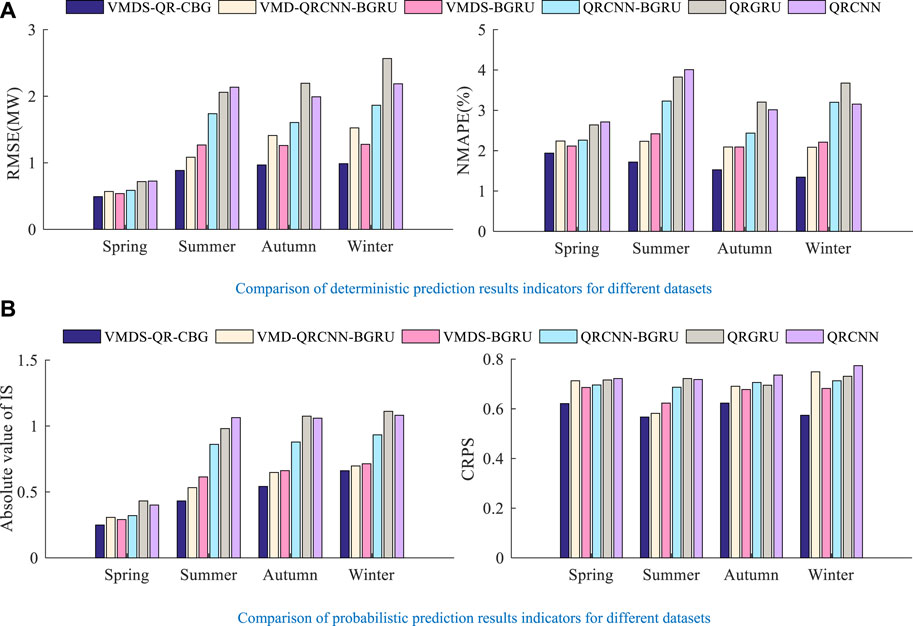
Data sets of different seasons are selected as the prediction objects to verify the versatility of the model in different meteorological conditions. Figure 7 shows the index comparison of the prediction results of different models for the four datasets. Both point predictors and probabilistic indicators of the proposed model are optimal in different datasets, which indicates that the proposed model has high generality.

FIGURE 7

FIGURE 7. Comparison of prediction results indicators for different datasets.

5 Conclusion

This study proposes a combined model of wind power probabilistic prediction based on combined decomposition and QR and CBG, namely VMDS-QR-CBG. The multi-channels input data of the model is constructed by VMDS, which can reduce the complexity of the data and improve the prediction ability of the model. CBG has powerful feature extraction ability, which can improve the accuracy of the whole model compared with the traditional model. Finally, QR and KDE combine VMDS and CBG to realize probabilistic prediction. Compared with the traditional model, VMDS-QR-CBG has better comprehensive performance in wind power prediction. The proposed combined model can achieve high reliability and acuity interval prediction and reliable and effective probabilistic prediction while ensuring the accuracy of point prediction. The proposed model combines a variety of methods, and the structure of the model is complex. The model can attempt to be optimized for larger scale wind power forecasts.

Data availability statement

The raw data supporting the conclusions of this article will be made available by the authors, without undue reservation.

Author contributions

Conceptualization, ZZ; methodology, ZZ and YX; original draft preparation, ZZ, YX, and JW; review and editing, ZZ, YL, and JG; supervision, HZ; project administration, ZZ, and HZ; funding acquisition, ZZ All authors have read and agreed to the published version of the manuscript.

Conflict of interest

The authors declare that the research was conducted in the absence of any commercial or financial relationships that could be construed as a potential conflict of interest.

Publisher’s note

All claims expressed in this article are solely those of the authors and do not necessarily represent those of their affiliated organizations, or those of the publisher, the editors and the reviewers. Any product that may be evaluated in this article, or claim that may be made by its manufacturer, is not guaranteed or endorsed by the publisher.

References

Amini, M. H., Kargarian, A., and Karabasoglu, O. (2016). ARIMA-based decoupled time series forecasting of electric vehicle charging demand for stochastic power system operation. Electr. Power Syst. Res. 140, 378390. doi:10.1016/j.epsr.2016.06.003

CrossRef Full Text | Google Scholar

Bokde, N., Feijoo, A., and Kulat, K. (2018). Analysis of differencing and decomposition preprocessing methods for wind speed prediction. Appl. Soft Comput. 71, 926938. doi:10.1016/j.asoc.2018.07.041

CrossRef Full Text | Google Scholar

Cheng, L., Zang, H., Wei, Z., Ding, T., Xu, R., and Sun, G. (2022). Short-term solar power prediction learning directly from satellite images with regions of interest. IEEE Trans. Sustain. Energy 13 (1), 629639. doi:10.1109/TSTE.2021.3123476

CrossRef Full Text | Google Scholar

Demolli, H., Dokuz, A. S., Ecemis, A., and Gokcek, M. (2019). Wind power forecasting based on daily wind speed data using machine learning algorithms. Energy Convers. Manag. 198, 111823. doi:10.1016/j.enconman.2019.111823

CrossRef Full Text | Google Scholar

Dragomiretskiy, K., and Zosso, D. (2014). Variational mode decomposition. IEEE Trans. Signal Process. 62, 531544. doi:10.1109/TSP.2013.2288675

CrossRef Full Text | Google Scholar

Erdem, E., and Shi, J. (2011). ARMA based approaches for forecasting the tuple of wind speed and direction. Appl. Energy 88, 14051414. doi:10.1016/j.apenergy.2010.10.031

CrossRef Full Text | Google Scholar

Georgilakis, P. (2008). Technical challenges associated with the integration of wind power into power systems. Renew. Sustain. Energy Rev. 12, 852863. doi:10.1016/j.rser.2006.10.007

CrossRef Full Text | Google Scholar

Global Wind Energy Council (GWEC) (2022). Global wind report 2022. Available at: https://gwec.net/global-wind-report-2022 (Accessed June 30, 2022).

Google Scholar

Han, L., Zhang, R. C., Wang, X. S., Bao, A., and Jing, H. (2019). Multi-step wind power forecast based on VMD-LSTM. IET Renew. Power Gener. 13, 16901700. doi:10.1049/iet-rpg.2018.5781

CrossRef Full Text | Google Scholar

He, Y. Y., and Li, H. Y. (2018). Probability density forecasting of wind power using quantile regression neural network and kernel density estimation. Energy Convers. Manag. 164, 374384. doi:10.1016/j.enconman.2018.03.010

CrossRef Full Text | Google Scholar

He, Y. Y., and Wang, Y. (2021). Short-term wind power prediction based on EEMD-LASSO-QRNN model. Appl. Soft Comput. 105, 107288. doi:10.1016/j.asoc.2021.107288

CrossRef Full Text | Google Scholar

Hong, Y. Y., and Satriani, T. R. A. (2020). Day-ahead spatiotemporal wind speed forecasting using robust design-based deep learning neural network. Energy 209, 118441. doi:10.1016/j.energy.2020.118441

CrossRef Full Text | Google Scholar

Hu, J. M., and Wang, J. Z. (2015). Short-term wind speed prediction using empirical wavelet transform and Gaussian process regression. Energy 93, 14561466. doi:10.1016/j.energy.2015.10.041

CrossRef Full Text | Google Scholar

Huang, R., Wang, X., Fei, F., Li, H., and Wu, E. (2022). Forecast method of distributed photovoltaic power generation based on EM-WS-CNN neural networks. Front. Energy Res. 10, 902722. doi:10.3389/fenrg.2022.902722

CrossRef Full Text | Google Scholar

Jin, H. P., Shi, L. X., Chen, X. G., Qian, B., and Yang, B. (2021). Probabilistic wind power forecasting using selective ensemble of finite mixture Gaussian process regression models. Renew. Energy 174 (1), 1. doi:10.1016/j.renene.2021.04.028

CrossRef Full Text | Google Scholar

Kisvari, A., Lin, Z., and Liu, X. L. (2021). Wind power forecasting - a data-driven method along with gated recurrent neural network. Renew. Energy 163, 18951909. doi:10.1016/j.renene.2020.10.119

CrossRef Full Text | Google Scholar

Liu, L. J., and Liang, Y. J. (2021). Wind power forecast optimization by integration of CFD and Kalman filtering. Energy Sources Part A Recovery Util. Environ. Eff. 43, 1880-1896. doi:10.1080/15567036.2019.1668080

CrossRef Full Text | Google Scholar

Liu, F. J., Li, C. S., Xu, Y. H., Tang, G., and Xie, Y. (2020). A new lower and upper bound estimation model using gradient descend training method for wind speed interval prediction. Wind Energy 24, 290304. doi:10.1002/we.2574

CrossRef Full Text | Google Scholar

Lv, J. Q., Zheng, X. D., Pawlak, M., Mo, W., and Miskowicz, M. (2021). Very short-term probabilistic wind power prediction using sparse machine learning and nonparametric density estimation algorithms. Renew. Energy 177, 181192. doi:10.1016/j.renene.2021.05.123

CrossRef Full Text | Google Scholar

Niu, Z. W., Yu, Z. Y., Tang, W. H., Wu, Q., and Reformat, M. (2020). Wind power forecasting using attention-based gated recurrent unit network. Energy 196, 117081. doi:10.1016/j.energy.2020.117081

CrossRef Full Text | Google Scholar

Oh, B. K., Glisic, B., Kim, Y., and Park, H. S. (2019). Convolutional neural network-based wind-induced response estimation model for tall buildings. Comput.-Aided. Civ. Inf. Eng. 34, 843858. doi:10.1111/mice.12476

CrossRef Full Text | Google Scholar

Peng, Z. Y., Peng, S., Fu, L. D., Lu, B., Tang, J., Wang, K., et al. (2020). A novel deep learning ensemble model with data denoising for short-term wind speed forecasting. Energy Convers. Manag. 207, 112524. doi:10.1016/j.enconman.2020.112524

CrossRef Full Text | Google Scholar

Peng, X. S., Wang, H. Y., Lang, J. X., Li, W., Xu, Q., Zhang, Z., et al. (2021). EALSTM-QR: Interval wind-power prediction model based on numerical weather prediction and deep learning. Energy 220, 119692. doi:10.1016/j.energy.2020.119692

CrossRef Full Text | Google Scholar

Ren, C., An, N., Wang, J. Z., Li, L., Hu, B., and Shang, D. (2014). Optimal parameters selection for BP neural network based on particle swarm optimization: a case study of wind speed forecasting. Knowledge-Based Syst. 56, 226239. doi:10.1016/j.knosys.2013.11.015

CrossRef Full Text | Google Scholar

Santhosh, M., Venkaiah, C., and Kumar, D. M. V. (2018). Ensemble empirical mode decomposition based adaptive wavelet neural network method for wind speed prediction. Energy Convers. Manag. 168, 482493. doi:10.1016/j.enconman.2018.04.099

CrossRef Full Text | Google Scholar

Sun, Z. X., Zhao, M. Y., Dong, Y., Cao, X., and Sun, H. (2021). Hybrid model with secondary decomposition, randomforest algorithm, clustering analysis and long short memory network principal computing for short-term wind power forecasting on multiple scales. Energy 221, 119848. doi:10.1016/j.energy.2021.119848

CrossRef Full Text | Google Scholar

Sun, Y., Huang, Y., and Yang, M. (2022). Ultra-short-term wind power interval prediction based on fluctuating process partitioning and quantile regression forest. Front. Energy Res. 10, 867719. doi:10.3389/fenrg.2022.867719

CrossRef Full Text | Google Scholar

Wang, H. Z., Li, G. Q., Wang, G. B., Peng, J. c., Jiang, H., and Liu, Y. T. (2017). Deep learning based ensemble approach for probabilistic wind power forecasting. Appl. Energy 188, 5670. doi:10.1016/j.apenergy.2016.11.111

CrossRef Full Text | Google Scholar

Wang, K. J., Qi, X. X., Liu, H. D., and Song, J. (2018). Deep belief network based k-means cluster approach for short-term wind power forecasting. Energy 165, 840852. doi:10.1016/j.energy.2018.09.118

CrossRef Full Text | Google Scholar

Wang, F., Xuan, Z., Zhen, Z., Li, K., Wang, T., and Shi, M. (2020). A day-ahead PV power forecasting method based on LSTM-RNN model and time correlation modification under partial daily pattern prediction framework. Energy Convers. Manag. 212, 112766. doi:10.1016/j.enconman.2020.112766

CrossRef Full Text | Google Scholar

Wang, F., Lu, X., Mei, S., Su, Y., Zhen, Z., Zou, Z., et al. (2021). A satellite image data based ultra-short-term solar PV power forecasting method considering cloud information from neighboring plant. Energy 238, 121946. doi:10.1016/j.energy.2021.121946

CrossRef Full Text | Google Scholar

Wang, Y., Wang, T., Chen, X., Zeng, X. J., Huang, J. J., and Tang, X. F. (2022). Short-term probability density function forecasting of industrial loads based on ConvLSTM-MDN. Front. Energy Res. 10, 891680. doi:10.3389/fenrg.2022.891680

CrossRef Full Text | Google Scholar

Wu, Y. K., Wu, Y. C., Hong, J. S., Phan, L. H., and Phan, Q. D. (2021). Probabilistic forecast of wind power generation with data processing and numerical weather predictions. IEEE Trans. Ind. Appl. 57, 3645. doi:10.1109/TIA.2020.3037264

CrossRef Full Text | Google Scholar

Yin, H., Ou, Z., Fu, J. J., Cai, Y., Chen, S., and Meng, A. (2021). A novel transfer learning approach for wind power prediction based on a serio-parallel deep learning architecture. Energy 234, 121271. doi:10.1016/j.energy.2021.121271

CrossRef Full Text | Google Scholar

Yu, C. J., Li, Y. L., and Zhang, M. J. (2017b). Comparative study on three new hybrid models using elman neural network and empirical mode decomposition based technologies improved by singular spectrum analysis for hour-ahead wind speed forecasting. Energy Convers. Manag. 147, 7585. doi:10.1016/j.enconman.2017.05.008

CrossRef Full Text | Google Scholar

Yu, C. J., Li, Y. L., and Zhang, M. J. (2017a). An improved wavelet transform using singular spectrum analysis for wind speed forecasting based on elman neural network. Energy Convers. Manag. 148, 895-904. doi:10.1016/j.enconman.2017.05.063

CrossRef Full Text | Google Scholar

Yu, C. J., Li, Y. L., Bao, Y. L., Tang, H., and Zhai, G. (2018). A novel framework for wind speed prediction based on recurrent neural networks and support vector machine. Energy Convers. Manag. 178, 137145. doi:10.1016/j.enconman.2018.10.008

CrossRef Full Text | Google Scholar

Yuan, X. H., Chen, C., Jiang, M., and Yuan, Y. (2019). Prediction interval of wind power using parameter optimized Beta distribution based LSTM model. Appl. Soft Comput. 82, 105550. doi:10.1016/j.asoc.2019.105550

CrossRef Full Text | Google Scholar

Zang, H., Cheng, L., Ding, T., Cheung, K. W., Wei, Z., and Sun, G. (2020a). Day-ahead photovoltaic power forecasting approach based on deep convolutional neural networks and meta learning. International Journal of Electrical Power and Energy Systems 118, 105790. doi:10.1016/j.ijepes.2019.105790

CrossRef Full Text | Google Scholar

Zang, H., Liu, L., Sun, L., Cheng, L., Wei, Z., and Sun, G. (2020b). Short-term global horizontal irradiance forecasting based on a hybrid CNN-LSTM model with spatiotemporal correlations. Renew. Energy 160, 2641. doi:10.1016/j.renene.2020.05.150

CrossRef Full Text | Google Scholar

Zang, H., Xu, R., Cheng, L., Ding, T., Liu, L., Wei, Z., et al. (2021). Residential load forecasting based on LSTM fusing self-attention mechanism with pooling. Energy 229, 120682. doi:10.1016/j.energy.2021.120682

CrossRef Full Text | Google Scholar

Zhang, Y. C., Liu, K. P., Qin, L., and An, X. (2016). Deterministic and probabilistic interval prediction for short-term wind power generation based on variational mode decomposition and machine learning methods. Energy Convers. Manag. 112, 208219. doi:10.1016/j.enconman.2016.01.023

CrossRef Full Text | Google Scholar

Zhang, Z. D., Qin, H., Liu, Y. Q., Yao, L., Yu, X., Lu, J., et al. (2019). Wind speed forecasting based on quantile regression minimal gated memory network and kernel density estimation. Energy Convers. Manag. 196, 13951409. doi:10.1016/j.enconman.2019.06.024

CrossRef Full Text | Google Scholar

Zhang, Y. G., Han, J. Y., Pan, G. F., Xu, Y., and Wang, F. (2021). A multi-stage predicting methodology based on data decomposition and error correction for ultra-short-term wind energy prediction. J. Clean. Prod. 292, 125981. doi:10.1016/j.jclepro.2021.125981

CrossRef Full Text | Google Scholar

Zhou, M., Wang, B., Guo, S., and Watada, J. (2021). Multi-objective prediction intervals for wind power forecast based on deep neural networks. Inf. Sci. 550, 207220. doi:10.1016/j.ins.2020.10.034

CrossRef Full Text | Google Scholar

Nomenclature

Indices

k Index of sub-sequence

t Index of time

l Index of layer

τ The quantile point

i Index of sample

p/q Index of channel

Parameters

X_IMF/X_IMFS/X_NWP The VMD components, SSA components and NWP data

X The historical wind power data input

X_f The fusion features

$u_k\left(t\right)$ The discrete sub-signal with different frequencies obtained by VMD

${\omega }_k$ The center frequencies of sub-signal

$\delta \left(t\right)$ The unit impulse function

$S\left(t\right)$ The original complex signal to be decomposed

$\lambda \left(t\right)$ The Lagrangian multiplier value at time t

$\beta$ The weight coefficient to ensure the accuracy of the reconstructed signal

$L(·)$ The joint objective function

${\Vert ·\Vert }_2$ The two-norm function

${\lambda }_i$ The i-th eigenvalue

U_i The eigenvector corresponding to the i-th eigenvalue

V_i The i-th principal component

$y_p^l$ The output vector of the p-th channel of the l-th layer

$x_q^{l-1}$ Input vector for the q-th channel of the l-1-th layer

$T_l$ / $T_{l-1}$ Number of channels for l-th layer and l-1-th layer

$v_n^l$ The l-th layer the n-th convolution kernel vector

$r(·)$ Activation function: rectified linear unit function

$W_{ij}$ The weight between the i-th neuron and the j-th neuron

$N_{l-1}$ The number of neurons in the l-1-th layer

$b_j^l$ The bias of the j-th neuron

$\sigma (·)$ Sigmoid activation function

$z_t$ / $r_t$ Output of update gate and reset gate

$h_t$ The state of the hidden layer at time t

$W_{zx}$ / $W_{zh}$/ $b_z$ Weights and biases of update gate

$W_{rx}$ / $W_{rh}$/ $b_r$ Weights and biases of reset gate

$\tanh$ Hyperbolic tangent function

X_in The historical data input

y The wind power forecast output

W/b The network weight and bias

$f(·)$ A nonlinear function reflecting the relationship between X_in and y

X_t The input of the t-th sample

y_t The actual value of the wind power of the t-th sample

f(W(τ),b(τ),X_i) The predicted value of wind power at τ-quantile

W(τ)/b(τ) The network parameters related to τ-quantile

${\rho }_{\tau }(·)$ The check function

$I(·)$ The indicative function

$\tilde{y}\left(\tau \right)$ The predicted value of wind power at the τ-quantile

B The bandwidth

$K(·)$ The kernel function

n The number of test samples

${\widehat{y}}_i$ The predicted values output by the i-th sample

$u_i^{\alpha }$ / $l_i^{\alpha }$ The lower and upper bounds of the prediction of the i-th sample

$\alpha$ The significance level

s The difference between the max value and the min value of the actual value

$P(·)$ The probability density function

$F(·)$ The cumulative density function