Probabilistic Prediction Intervals of Wind Speed Based on Explainable Neural Network

With the rapid growth of wind power penetration into modern power grids, wind speed forecasting plays an increasingly significant role in the planning and operation of electric power and energy systems. However, the existing wind speed forecasting methods are modeled as black boxes, which are very complicated and cannot be written down explicitly due to the complex fluctuation characteristics of wind speed series. To this end, this study proposes a novel direct method based on an explainable neural network (xNN) for deterministic and probabilistic wind speed forecasting. It can theoretically extract the nonlinear mapping features in wind speed, thereby providing a clear explanation of the relationship between the input and the output of the forecasting model. Then, the uncertainties in wind speed are statistically synthesized via the kernel density estimation method. Finally, we use wind speed data from real wind farms in Belgium to verify the feasibility and effectiveness of the proposed method. The simulation results demonstrate that it is not only able to accurately extract the non-stationary feature in the wind speed series but also superior to other benchmark algorithms in prediction accuracy. Therefore, the proposed method has a high potential for practical applications in real electric power and energy systems.

1 Introduction

Due to the concerns about reserves of fossil fuels, renewable energy has become an essential part of global energy (Wang et al., 2019a). Among renewable energy, wind energy is recognized as clean energy with a high conversion rate, large-scale development, and rich resources (Long et al., 2022). Moreover, wind energy can reduce greenhouse gas emissions to relieve the energy systems effectively. Therefore, the level of wind power penetration into modern power grids has correspondingly increased in the past decades (Anjaiah et al., 2022). However, the randomness, volatility, and reverse load characteristics of wind power will definitely aggravate the power supply–consumption imbalance, thus bringing great challenges to the economic operation, stability, and security of the electric energy system (Desai and Makwana, 2021). Wind speed forecasting affects not only the reserve capacity and maintenance plan of the energy system but also energy market transactions and charge and discharge plans of the storage stations (Wang et al., 2018). Therefore, accurate wind speed forecasting is crucial for availably dispatching wind power resources.

Traditionally, wind speed prediction methods focus on the deterministic forecast, namely point predictions, which have strong stability and accurately describe the nature of fluctuation of wind speed (Tang et al., 2020). However, it fails to estimate the uncertainties associated with a given prediction of wind speed predictions. These uncertainties play a key role in improving the economic benefits of day-ahead energy bidding and reserve scheduling (Fu, 2022). Therefore, it is necessary to develop probabilistic prediction tools with consideration of the uncertainty in wind speed predictions, which can help dispatchers prepare for possible scenarios in advance (Haque et al., 2014), thus reducing the risk of power system control and management.

In recent years, considerable research has been conducted to obtain prediction intervals (PIs) through probabilistic wind speed forecasts (Xydas et al., 2017). So far, it can be mainly divided into three categories: physical modeling method, statistical model, and hybrid artificial intelligence method (Khodayar et al., 2019). The essence of physical modeling methods is to establish an accurate mathematical model by assembling various meteorological variables to obtain the forecast distribution and estimate the uncertainty in the forecast (Zhao et al., 2018). The statistical method attempts to establish the relationship between future wind power and historical samples to minimize the error (Scheu et al., 2017; Wang Y. et al., 2019; Pokhrel and Seo, 2021). Investigating the uncertainty in prediction for wind power based on the statistical analysis of wind speed prediction and errors of the nonlinear power curve is presented in Zhao et al. (2016). Zhang et al. (2015) proposed a kernel density estimation method based on logarithmic transformation to estimate the uncertainty in wind energy. Compared with the other two methods, artificial intelligence has been developed prosperously due to its potential ability in data mining and feature extraction (Liu et al., 2013; Aurore et al., 2020; Madhiarasan, 2020). Besides, many studies have been done on the combinations of these methods recently. Wan et al. (2017) combined the extreme learning machine (ELM) and QR to directly generate quantiles of different proportions. Wang et al. (2016) proposed a hybrid statistical approach in combination with wavelet transform, deep belief network and spline QR to completely extract nonlinear features of each frequency, validated by Bornholm Island wind farm. Moreover, Wang et al. (2017) proposed an ensemble of wavelet transforms and a convolutional neural network for probabilistic wind speed forecasts and separately identified the model misspecification and data noise. The probability distribution of wind power data can be expressed by statistical models. In addition, the hybrid algorithm of neural network and optimization algorithms are widely used in probabilistic predictions. Wan et al. (2014) used particle swarm optimization (PSO) to directly optimize the output weights of ELM based on the objective function while the network outputs PIs with different PI confidence levels (PICP). Wang et al. (2020a) proposed a wind power interval prediction model based on a spiking neural network (SNN) and used a group search optimizer introduced and redesigned to optimize the parameters of SNN and directly generate the prediction intervals. Thus, it can be concluded that neural networks (NNs) play a significant role in the field of probabilistic predictions.

However, in the decision-making process, these models fail to judge whether NNs have made decisions on the basis of general features or random features in the training data (Yildiz et al., 2021). To date, an explainable probabilistic prediction model designed for wind speed forecasting has not yet been considered in the published literature. Therefore, this study aims to fill this gap and proposes a new explainable probabilistic prediction model for wind speed forecasting. This work, which investigates a deep wind speed forecasting framework and a hybrid intelligent approach based on xNN, bootstrap method, and KDE, is originally proposed to enhance prediction efficiency and provide a clear explanation of the relationship between the input of this model and its output. The main advantage of the proposed probabilistic prediction framework is that it can express how the input variables affect the output results through mathematical formulations. By analyzing the behavior of the model, we can understand which features of wind act as the main factors affecting the prediction accuracy and determine whether the input-output relationship of NN is consistent with the common knowledge in the wind energy system. By comparing with the existing methods, this approach takes the measured data of wind farms as the micro-scale NWP data, and it focuses on the following key aspects:

(1) For the first time, a new explainable prediction NN is originally proposed for wind speed forecast, which can learn the interpretable features of wind speed and express how the input variables affect the result by formulation.

(2) Based on the aforementioned discussion, this study proposed a deterministic forecasting model, which introduces the bootstrap method to reduce the noise of training data and the misspecification of the NN model for regression, so it is called B-xNNs.

(3) The KDE can avoid inaccurate predictions caused by the unreasonable assumption error distribution independently without setting hypotheses for the wind power error distribution in advance. According to the prediction results from B-xNNs, the uncertainty of prediction is devoted to obtaining the probability prediction results with high reliability.

(4) The proposed method has been tested using the measurement data of a wind farm in Belgium after comprehensively evaluating the feasibility of the forecasting results. The effectiveness and interpretability of the proposed approach have been demonstrated by the results.

The rest of this research is organized as follows: Section 2 introduces a probabilistic forecasting formulation based on xNN. Section 3 describes PIs evaluation indices including reliability and sharpness. In Section 4, comprehensive numerical studies are implemented and the superiority of the proposed method is demonstrated. Finally, the conclusion is drawn in Section 5.

2 Probabilistic Forecasting Formulation Based on Explainable Neural Network

2.1 Explainable Neural Network

This section introduces the structure and mathematical model of xNN, as presented in the left half of Figure 1. It is a feed-forward neural network with one input layer, two linear layers, and one nonlinear layer with Legendre polynomial. The mathematical models of the four layers are given below.

FIGURE 1

FIGURE 1. Probabilistic forecasting framework based on B-xNNs.

Given the datasets with N arbitrary distinct samples $D_t={\left\{\left({\mathbf{x}}_i,{\mathbf{t}}_i\right)\right\}}_{i=1}^N$, where t_i is the wind speed of ith time and X_i is the input vector including historical wind speed, wind direction and radiation, and NWP, it can be expressed as ${\mathbf{X}}_i={\left[x_{i1},x_{i2},\mathrm{...},x_{in}\right]}^T$. Therefore, the input layer is responsible for inputting wind power-related features and time series data into the xNN structure. As shown in Figure 1, the input layer is fully connected to the first hidden layer and consists of K nodes. In this layer, a linear activation function is employed, so each neuron in this layer learns a linear combination of the input features and time series data. Equation 1 denotes the input weight of the jth node, expressed by

${\beta }_j=\left[\begin{array}{c}{\omega }_{1j}\\ {\omega }_{2j}\\ \mathrm{...}\\ {\omega }_{nj}\end{array}\right].(1)$

Therefore, the output of jth node of this layer can be expressed by the following equation:

$V_j={\beta }_j^{T}X={\displaystyle \sum _{i=1}^n{\omega }_{ij}{X}_i}.(2)$

The second hidden layer is used to learn the ridge functions g_j(·), which is taken as the activation function of the nonlinear neuron in this layer. As shown in Figure 1, connections between the first hidden layer and the second one can cause a potentially nonlinear transformation of the input. The output of jth node of the second hidden layer is expressed as

$h_j={\text{g}}_j\left(V_j\right)=g_j\left({\beta }_j^{T}X\right).(3)$

As shown in Figure 1, the output layer consists of a single node using a linear activation function. Therefore, the output layer is a linear combination of the second hidden layer to ensure that all features of the previous layer can be learned.

Ridge function is taken as the activation function of the nonlinear neuron in this layer as follows:

$g_{jK}=\frac{1}{K!}{\left({\beta }_j^{T}X\right)}^K,(4)$

where g_jK represents an activation function of the Kth neural in the nonlinear layer. Therefore, the output of the last layer can be expressed as

$f==\frac{1}{i!}{\displaystyle \sum _{i=1}^K{\displaystyle \sum _{j=1}^n{\gamma }_j{\left({\beta }_j^{T}X\right)}^i}}+\mu ,(5)$

where $\gamma$ is the weight of the second hidden layer and μ is the bias of the output layer. It can be seen from Eq. 5 that xNN is an additive index model based on the neural network, which allows direct calculation of partial derivatives of the function. This enables xNN to perform derivative-based analysis techniques without relying on finite difference approximation (Yang et al., 2021). The effect of input parameters on the output can be analyzed theoretically by Eq. 5 to provide straightforward explanations of how the model uses the input features to make predictions in wind speed.

2.2 Uncertainty in xNN Probabilistic Forecasting Model

The uncertainty of the model is the primary reason for the uncertainty of xNN probabilistic forecasting. Specifically, these uncertainties may be caused by over-training, model misspecification, and high sensitivity to initial parameters, among others (Guignard et al., 2021). Although the global minimum value is reached, the uncertainty of the xNN model structure will also cause non-negligible errors. In the research of wind power generation prediction, it is impossible to ensure consistent generalization performance of xNN for the unknown future because of the limited samples. Namely, it is impossible to find perfect parameters and structures to eliminate the uncertainty of the model. These factors are collectively referred to as xNN model uncertainty. Therefore, to reduce the uncertainty of wind speed forecasting and produce accurate estimation, the development of prediction for the xNN forecasting framework is based on the bootstrap method.

Bootstrap is regarded as a general method of statistical inference based on establishing a sampling distribution by uniform sampling replacing from the raw data (Efron and Tibshirani, 1993). In order to reduce the uncertainty of wind speed forecasting, we train B-xNNs on particular bootstrap samples to adjust the network parameters, whereas the model misspecification and data noise can cancel each other through this process (Chen et al., 2018). The flowchart of the proposed structure is described in detail in Figure 2. Based on historical wind speed data, we create an original training dataset at first. Then, the original training data are evenly sampled and replaced to generate bootstrapped pairs devoted to the input of the xNN. Afterward, M xNNs will be derived from wind power forecasting by training based on the M bootstrap replicates. Its average output is taken as the estimation of the final regression.

FIGURE 2

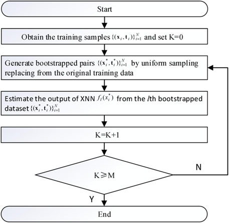
FIGURE 2. Flowchart of Pairs bootstrap based on xNN.

2.3 Prediction Intervals Construction Based on xNN

The construction of new wind power prediction intervals is proposed in this section. The overall structure of the xNN-based forecasting framework is shown in Figure 1, and wind power time series data are used as the input of the proposed method. Lower bound $L_t^{\alpha }$ and upper bound $U_t^{\alpha }$ of the prediction interval are the outputs of the proposed method with its corresponding confidence levels of 100(1-α)%.

2.3.1 Kernel Density Estimation

As shown in Figure 1, to estimate the optimal prediction intervals statistically, the proposed wind power probabilistic forecasting method adopts KDE to fit the final regression errors of wind speed obtained by the xNNs. Wang et al. (2019c) presented that KDE can be used as an effective mathematical tool to study the characteristics of data distribution based on the distribution-free principle instead of using prior distributions. Therefore, the impact of the hypothesis in wind speed forecasting error on the prediction accuracy can be appropriately mitigated. Given the wind speed prediction error datasets $S=\left\{s_1,s_2,s_3,\mathrm{...},s_n\right\}$ with n arbitrary distinct samples, the probability density function (PDF) is shown as

$\stackrel{\text{∼}}{f}\left(s,h\right)=\frac{1}{nh}{\displaystyle \sum _{i=1}^{n}K\left(\frac{s-s_i}{h}\right)},(6)$

where h represents bandwidth for determining the width of the distribution interval of the prediction error and the K(.) termed the kernel function, and s_i is the ith sample of wind speed prediction error. Common kernel functions include Uniform kernel, Gamma kernel, Epanechnikov kernel, and Gaussian kernel. In this study, the Gaussian kernel function is selected as the kernel function, expressed as follows:

$K\left(s\right)=\frac{1}{\sqrt{2\pi }}\exp \left(\frac{-s^2}{2}\right).(7)$

Therefore, the PDF can be transformed into the following equation:

$\stackrel{\sim }{f}\left(s,h\right)=\frac{1}{\sqrt{2\pi }nh}{\displaystyle \sum _{i=1}^n\exp \left(-\frac{1}{2}{\left(\frac{s-s_i}{h}\right)}^2\right)}.(8)$

The error can be minimized by selecting the appropriate bandwidth h, which controls the balance between the bias and variance in the results. So far, there are some studies on the mean squared error (MSE), integrated squared error (ISE), and mean integrated squared error (MISE) criteria to select h (Duan et al., 2021). By comparing with the MISE method, the other two methods require higher accuracy for single-point prediction. MISE can be expressed by the following equations:

$M\left(h\right)=E{\displaystyle \int {\tilde{f}}_h}{\left(\left(s\right)-f\left(s\right)\right)}^{2}ds={{\displaystyle \int \left(E{\tilde{f}}_h\left(s\right)-f\left(s\right)\right)}}^{2}ds+{\displaystyle \int \mathrm{var}{\tilde{f}}_h\left(s\right)ds},(9)$

$M\left(h\right)=\frac{h^4}{4}{\displaystyle \int s^2}K\left(s\right)dx{\displaystyle \int {\left\{f^{\prime \prime }\left(s\right)\right\}}^2}ds+\frac{1}{nh}{\displaystyle \int K^2}\left(s\right)ds+o\left(\frac{1}{nh}+h^4\right),(10)$

where $\mathrm{var}{\tilde{f}}_h\left(s\right)$ is the variance of the KDE. According to Xydas et al. (2017), we can obtain the asymptotic mean integrated squared error (AMISE):

$AMISE=\frac{h^4}{4}{\displaystyle \int s^2}K\left(s\right)dx{\displaystyle \int {\left\{f^{\prime \prime }\left(s\right)\right\}}^2}ds+\frac{1}{nh}{\displaystyle \int K^2}\left(s\right)ds.(11)$

According to Xin et al. (2020), the optimal bandwidth can be expressed by

$h_{op}={\left(\frac{R\left(K\right)}{T^2\left(K\right)R\left(f^{"}\right)n}\right)}^{\frac{1}{5}},(12)$

where R(K) is the square integral of kernel function K(s) and T(K) is the second moment of kernel function K(.), represented, respectively, as $R\left(K\right)={\displaystyle \int K^2\left(x\right)dx}$ and $T\left(K\right)={\displaystyle \int x^{2}K\left(x\right)dx}$.

The normal distribution with variance σ² is used in the reference distribution of the unknown probability density function. Thus, Eq. 12 can be transformed into

$h_{op}={\left(4\pi \right)}^{-\frac{1}{10}}\frac{3}{8}{\pi }^{-\frac{1}{2}}\sigma n^{-\frac{1}{5}}={\left(\frac{4}{3}\right)}^{\frac{1}{5}}\sigma n^{-\frac{1}{5}}.(13)$

It should be noted that inaccurate estimates will be obtained when the error probability density is away from the normal distribution. Therefore, the trial-and-error method is used to select the appropriate bandwidth (Yang et al., 2018). The proposed modification of the optimal bandwidth h_op is to deal with unimodal and bimodal densities, expressed as

$h_{op}=0.9\min \left(\sigma ,\frac{E_{IQR}}{1.34}\right)n^{-\frac{1}{5}},(14)$

where E_IQR is the difference between 75% and 25% of the sample quantile. In Eq. 14, a discrete set near the h_op has been defined, and the trial-and-error method is used to select the appropriate bandwidth in this discrete set. The fluctuation range of prediction errors at the confidence level of 100(1-α)% is obtained by the corresponding cumulative distribution function (CDF) as follows:

$\begin{array}{cc}{I}_e\left(\alpha \right)=\left[F\left(\alpha \right),F\left(1-\alpha /2\right)\right]& \left(0<\alpha <1\right)\end{array}.(15)$

Therefore, the 100(1-α)% confidence level PI of the measured target is a stochastic interval of wind power, expressed by

$\left[{\tilde{L}}_i^{\left(\alpha \right)}\left({\mathbf{x}}_i\right),{\tilde{U}}_i^{\left(\alpha \right)}\left({\mathbf{x}}_i\right)\right]=\left[y_{i,pre}^{\left(\alpha \right)}-F^{\text{*}}\left(\alpha \right),y_{i,pre}^{\left(\alpha \right)}+F^{\text{*}}\left(1-\alpha /2\right)\right],(16)$

$y_{i,pre}^{\left(\alpha \right)}\in \left[{\tilde{L}}_i^{\left(\alpha \right)}\left({\mathbf{x}}_i\right),{\tilde{U}}_i^{\left(\alpha \right)}\left({\mathbf{x}}_i\right)\right],(17)$

where $y_{i,pre}^{\left(\alpha \right)}$ is the prediction result of the B-xNNs at the ith sample under confidence levels of 100(1-α)%.

2.3.2 Probabilistic Forecasting Framework Based on xNN

The flowchart of the xNN-based probabilistic forecasting framework is mainly divided into three parts. The first part is to train the M xNNs based on the training dataset, saving the model with approximate optimal structure. More specifically, the training dataset based on the input dataset within the historical wind speed data and NPWs is devoted to generating M bootstrap replicates. All parameters in B-xNNs are randomly initialized and updated based on the layer-wise pre-training process and fine-tuning process until they all are converged. In the second part, the essential idea of the process is to obtain the optimal parameters of the KDE. In order to obtain the error dataset, we verify the forecasting performance of B-xNNs on the validation set. Then, compared with the true regression, the error of model misspecification uncertainty can be estimated from the B-xNNs. Subsequently, the error dataset is adopted to calculate cumulative distribution, and the probabilistic wind speed forecasting model is statistically established based on the KDE. Therefore, the wind speed forecasting uncertainties can thus be probabilistically represented as a set of quantiles. In the last part, the testing dataset is used to verify the probabilistic forecasting performance framework. The overall schematic diagram is illustrated in Figure 3.

FIGURE 3

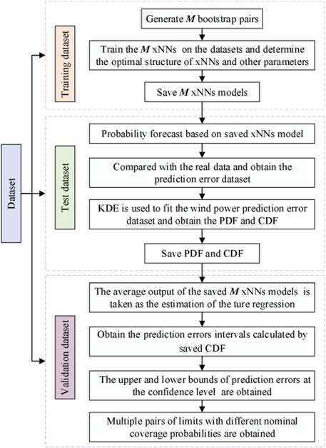
FIGURE 3. Flowchart of probabilistic forecasting based on xNN.

3 Performance Evaluation Metrics

3.1 Deterministic Forecast Evaluation

In order to comprehensively assess the overall prediction performance of B-xNNs, three widely used metrics in statistics are employed: mean absolute error (MAE), mean absolute percentage error (MAPE), and root mean square error (RMSE) (Xu et al., 2021). Calculation formulas for these evaluation indicators are as follows:

$MAE=\frac{1}{N}{\displaystyle \sum _{i=1}^N\left|\overline{y_i}-y_i\right|},(18)$

$MAPE=\frac{100\%}{N}{\displaystyle \sum _{i=1}^N\left|\frac{\overline{y_i}-y_i}{y_i}\right|},(19)$

$RMSE=\sqrt{\frac{1}{N}{{\displaystyle \sum _{i=1}^N\left|\overline{y_i}-y_i\right|}}^2},(20)$

where $\overline{y_i}$ represents the predicted value of the input samples generated by the B-xNNs, $y_i$ represents the true regression, and N represents the number of samples.

3.2 PI-Based Forecast Evaluation

According to the definition of prediction interval (PI), the target t_i with PI nominal confidence (PINC) 100(1-α)% is in the constructed prediction interval:

$t_i\in \left[{\tilde{L}}_t^{\left(\alpha \right)}\left({\mathbf{x}}_i\right),{\tilde{U}}_t^{\left(\alpha \right)}\left({\mathbf{x}}_i\right)\right],(21)$

where ${\tilde{L}}_t^{\left(\alpha \right)}\left({\mathbf{x}}_i\right)$ and ${\tilde{U}}_t^{\left(\alpha \right)}\left({\mathbf{x}}_i\right)$ are the lower and upper bounds of PI with nominal confidence of the future target t_i.

As a major attribute of probabilistic prediction models, reliability is denoted by the probability of target between prediction intervals because low reliability will lead to systematic bias in subsequent decision problems (Li et al., 2016). PI coverage probability (PICP) is used to evaluate the reliability of the prediction interval, which is defined by

$PICP=\frac{1}{N_t}{{\displaystyle \sum _{i=1}^{N_t}{d}_i}}^{\left(\alpha \right)},(22)$

where N_t is the number of the sample and d_i is the Boolean variable, expressed by

$d_i=\{\begin{array}{cc}0& ti\notin \left[{\tilde{L}}_t^{\left(\alpha \right)}\left({\mathbf{x}}_i\right),{\tilde{U}}_t^{\left(\alpha \right)}\left({\mathbf{x}}_i\right)\right]\\ 1& ti\in \left[{\tilde{L}}_t^{\left(\alpha \right)}\left({\mathbf{x}}_i\right),{\tilde{U}}_t^{\left(\alpha \right)}\left({\mathbf{x}}_i\right)\right]\end{array}.(23)$

The coverage probability of derived PIs is expected to approach the nominal level of confidence asymptotically as close as possible. Average coverage error (ACE), therefore, can be used for the evaluation of the PIs, defined by

$A_t^{\left(\alpha \right)}=PICP-PINC.(24)$

The interval score index is served to evaluate the quality of the prediction interval by rewarding narrower PIs and punishing wider PIs (Wan et al., 2014), expressed as follows:

$S_t^{\left(\alpha \right)}\left({\mathbf{x}}_i\right)=\{\begin{array}{ccc}-\alpha I_t^{\left(\alpha \right)}\left({\mathbf{x}}_i\right)-2\left[{\tilde{L}}_t^{\left(\alpha \right)}\left({\mathbf{x}}_i\right)-t_i\right]& ti<{\tilde{L}}_t^{\left(\alpha \right)}\left({\mathbf{x}}_i\right)& \mathrm{ }\\ -\alpha I_t^{\left(\alpha \right)}\left({\mathbf{x}}_i\right)& t_i\in \left[{\tilde{L}}_t^{\left(\alpha \right)}\left({\mathbf{x}}_i\right),{\tilde{U}}_t^{\left(\alpha \right)}\left({\mathbf{x}}_i\right)\right]& \mathrm{ }\\ -\alpha I_t^{\left(\alpha \right)}\left({\mathbf{x}}_i\right)-2\left[t_i-{\tilde{U}}_t^{\left(\alpha \right)}\left({\mathbf{x}}_i\right)\right]& t_i>{\tilde{U}}_t^{\left(\alpha \right)}\left({\mathbf{x}}_i\right)& \mathrm{ }\end{array}.(25)$

The average score can be obtained by

${\overline{S}}_t^{\left(\alpha \right)}=\frac{1}{N_t}{\displaystyle \sum _{i=1}^{N_t}{S}_t^{\left(\alpha \right)}\left({\mathbf{x}}_i\right)}.(26)$

Obviously, simply increasing or decreasing the width between the bounds of PI can easily lead to high reliability. However, the resultant PIs are useless in practice because of the degradation of interval sharpness (IS) (Guignard et al., 2021). Therefore, sharper PIs have higher quality and would be preferred under the condition of high reliability.

3.3 Interpretability of the Proposed Approach

According to the analysis in Section 2, the final output of the B-xNNs can be expressed as

$\overline{f}==\frac{1}{Mi!}{\displaystyle \sum _{m=1}^M{\displaystyle \sum _{i=1}^K{\displaystyle \sum _{j=1}^n{\gamma }_j{\left({\beta }_j^{T}X\right)}^i}}+\mu },(27)$

which is actually a nonlinear mapping function of the input vector X. Therefore, the new B-xNNs model for wind speed prediction is proposed to quantitatively analyze how the input variables of B-xNNs affect the prediction results by explicit formulation. In the process of probabilistic forecasting, we can obtain the optimal parameters of the KDE by estimating the uncertainty of B-xNNs prediction. It can be seen from Eq. 8 that the input-output relationship of PDF is actually a polynomial of the error data S. Obviously, the proposed probabilistic forecasting structure in Figure 1 is designed to explicitly learn the measured data of wind farms and the prediction interval with different confidence relationship. From Eqs 8 and 27, we can not only extract the interpretable features in wind speed but also theoretically analyze how the input variables affect the interval prediction results. It means that the corresponding relationship can be found from the input characteristics for the PIs with different confidence levels. Therefore, the whole probabilistic prediction framework is promising and attractive due to its interpretability and explainability.

4 Case Studies

4.1 Experiment Data Description

In this study, the proposed approach has been comprehensively tested and benchmarked on wind speed datasets from a Belgian transmission company called Elia. The Belgian coordinate system, located in 50°51′ north latitude and 4°21′ east longitude, has abundant wind energy resources and its wind power installation capacity is large (Wang et al., 2020b). Due to the high complexity of chaotic climate systems, weather conditions are quite different in the four seasons, which will bring a high level of uncertainties in wind speed. Therefore, four different prediction models in the same framework and seasonal datasets are considered in this experimental test. To ensure the effectiveness of generation and reserve dispatches, we adopt a short-term forecast. In addition, models are constructed separately for different seasons. The entire wind speed datasets are divided into four groups and each group covers one season of data, respectively. In each dataset, data are divided into training, verification, and test sets, with percentages of 78%, 11%, and 11%, respectively. Besides, in order to ensure the accuracy and sharpness of the prediction, the parameter M of B-xNNs is selected as 150. In other words, 150 bootstrap replicates are used to generate PIs in the case study.

4.2 Experimental Results and Analysis of B-xNNs

To fully validate the effectiveness of the proposed algorithm, the results are compared with the backpropagation neural network (BPNN) and the long short-term memory (LSTM). The detailed testing results, including the regression evaluation indices MAE, MAPE, and RMSE, are given in Table 1. The minimum and maximum MAE index values of the proposed method are 0.4512 and 0.5831, respectively, with an average of 0.5027. The MAE indices of LSTM and BPNN varied from 0.6236 to 0.7852 and from 0.6859 to 0.7652, with average values of 0.7013 and 0.7232, respectively. Compared to LSTM and BPNN, the MAPE has been evenly improved by 36.72% and 41.87%, respectively, and RMSE by 32.04% and 33.14%, respectively. The regression indexes of the proposed prediction framework are significantly better than the prediction results of the BPNN and LSTM algorithms. The above numerical simulation results show that the proposed prediction framework shows good prediction performance in all four seasons, so it has strong forecasting robustness.

TABLE 1

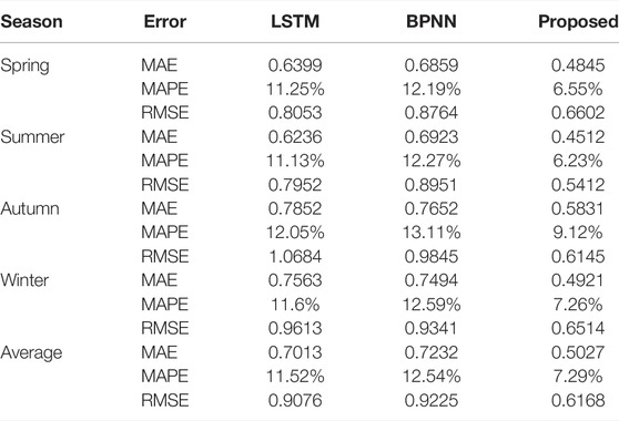
TABLE 1. Deterministic 1 h ahead statistical prediction results of the four methods.

Moreover, to graphically demonstrate the privilege of the proposed approach, the prediction results of different methods are presented in Figures 4–7, respectively. The curves in different colors represent the prediction results using different algorithms. It can be seen that the results from the proposed approach and the real values almost overlap in all four seasons, indicating that the estimated values are closest to the real data. The prediction results of BPNN and LSTM algorithms have relatively large forecasting errors. Therefore, the comparative results demonstrate that the proposed hybrid algorithm exhibits the best point forecast performances in all four seasons and thus shows the best prediction capability over the benchmarks. In addition, the results also show that the LSTM outperforms the BPNN 1-h ahead forecasts, which is consistent with the results presented in Wang et al. (2020b). This result is due to the high nonlinearity, complexity, and non-smoothness exhibited in short-time wind speed series. These dynamics cannot be extracted effectively by shallow NN models, such as BPNN.

FIGURE 4

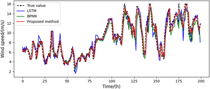
FIGURE 4. Prediction results of three different methods in spring.

FIGURE 5

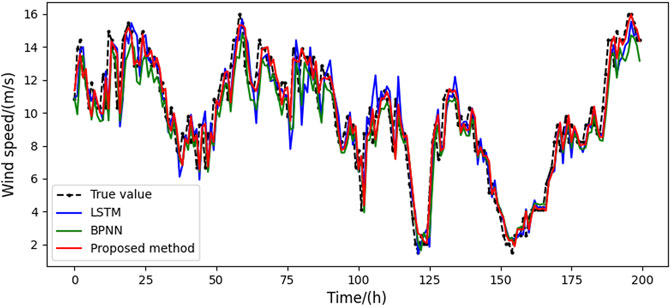
FIGURE 5. Prediction results of three different methods in summer.

FIGURE 6

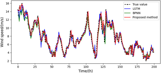
FIGURE 6. Prediction results of three different methods in autumn.

FIGURE 7

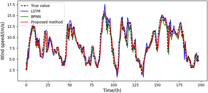
FIGURE 7. Prediction results of three different methods in winter.

4.3 Experimental Results and Analysis of the Proposed Probabilistic Method

This section evaluates the effectiveness of the proposed probabilistic approach. According to Section 2.3, we have drawn probability density distribution and corresponding cumulative probability distributions with prediction error results, as shown in Figures 8–11. It can be seen that seasonal segmenting and fitting are feasible to describe the probability distribution of prediction errors in different seasons. In Figures 10, 11, the upper and lower quintiles within different confidence levels 95%, 90%, and 80% are shown with α/2 = 2.25%, α/2 = 5%, and α/2 = 10%, respectively. Therefore, the upper and lower bounds of prediction errors at the confidence level of 100(1-α)% are obtained on the solid basis of the CDF. The fluctuation effect of the wind power prediction interval within spring and autumn is shown in Figures 12 and 13, manifesting that the width of the prediction interval decreases whereas the interval coverage and confidence level decrease. Figures 12 and 13 show that the wind speed data are perfectly enclosed by the PIs generated by the proposed method, indicating that the probabilistic performance criteria for the samples are satisfactory. Besides, although the non-stationary characteristics of wind speed series are displayed in Figures 12 and 13, the PIs still have high coverage, suggesting that the proposed prediction framework can construct high-quality PIs for wind speed datasets at a wide range of confidence levels. Considering that some generated PIs may have abnormal values beyond the possible generation range of the wind farms, the resultant predictive densities have been censored to concentrate on the probability of abnormal conditions mass on the bounds.

FIGURE 8

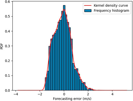
FIGURE 8. PDF of predicted error within spring.

FIGURE 9

FIGURE 9. PDF of predicted error within autumn.

FIGURE 10

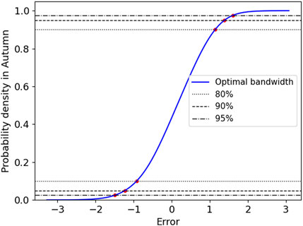
FIGURE 10. CDF of predicted error within spring.

FIGURE 11

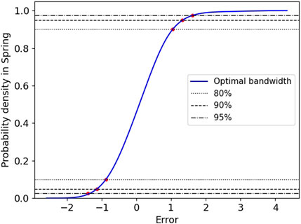
FIGURE 11. CDF of predicted error within autumn.

FIGURE 12

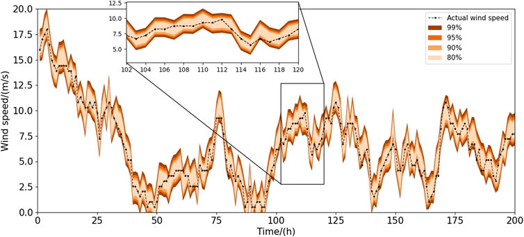
FIGURE 12. Interval prediction of different confidence within spring.

FIGURE 13

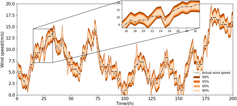
FIGURE 13. Interval prediction of different confidence within autumn.

According to Section 3.2, two indices, ACE and IS, are used in the literature to measure the probabilistic performance. Regarding ACE and IS, high-confidence levels of PINC 100(1-α)% ranging from 90% to 99% are generally considered because of the high reliability required in power system optimization and operation (Wang et al., 2022). These two probabilistic indices and their corresponding PICP are tabulated in Table 2. In all four seasons, the ACE of the proposed approach exhibits the lowest deviations to the nominal confidence levels, especially in the case of higher confidence levels of 95% and 99%. Quantitatively, the average of ACE using the proposed approach is 0.5717%; the average of IS is between −6.62% and −1.08%; and the average score is −3.73%. The IS bias increases as the PINC increases because it is a punishment system for a wide range. These results prove that the reliability errors between the observed probability and nominal confidence from the proposed approach are at a minimum and further indicate that the proposed approach exhibits higher prediction reliability.

TABLE 2

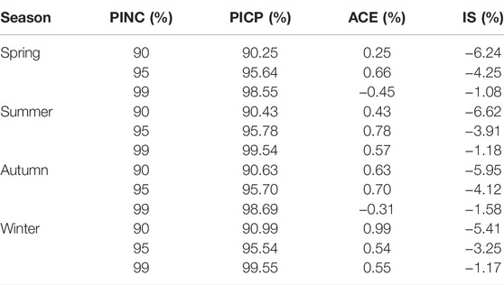
TABLE 2. Probabilistic forecasting error in different seasons.

To further demonstrate the effectiveness and feasibility of the proposed probabilistic prediction approach, three other PI forecasting methods, namely, persistence method, LSTM + QR, and BP + QR, are employed to compute PIs using the same training and testing data for benchmarking, and the numerical results are tabulated in Figures 14 and 15. Statistically, when PINC is 95%, the IS of the quantiles obtained from the persistence, LSTM, and BPNN ranges from −5.95% to −4.92%, −5.22% to −4.11%, and −5.68% to −4.78%, whereas the proposed method ranges from a low of −4.25% to a high of −3.25%. Particularly, the proposed method has an IS of −3.25%, which is significantly better than those of the persistence, LSTM, and BPNN algorithms in all four seasons. In addition, IS of the proposed method has a minimum of −1.28% and a maximum of −1.18% for the whole year, and the average value is 1.23%. Compared to the three benchmarks, IS performances have been evenly improved by 33.42%, 34.02%, and 40.10% when PINC is 99%. Therefore, it is clear from these numerical results that the proposed approach outperforms benchmarking algorithms in terms of seasons and prediction interval confidence.

FIGURE 14

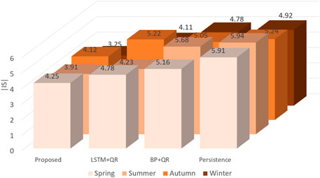
FIGURE 14. IS performance with PINC 95%.

FIGURE 15

FIGURE 15. IS performance with PINC 99%.

ACE and IS are two typical metrics used to evaluate the effectiveness and are satisfactory for probabilistic prediction. Based on the above results, it is evident that the proposed probabilistic approach outperforms the three benchmarks not only from the viewpoint of reliability and sharpness but also from the perspective of overall skills.

4.4 Explainability of the Proposed Method

The mapping relationship would become difficult to interpret in the NNs-based model due to the complexity introduced by typical unreadable functions, such as sigmoid. However, by analyzing the internal parameters of the model in the B-xNNs, the mapping relationship between the input and output of the wind speed prediction model can be written in a uniform equation as follows:

$f^{\left(i\right)}=C_3^{\left(i\right)}{\left(P_3^{\left(i\right)}{X}^T\right)}^3+C_2^{\left(i\right)}{\left(P_2^{\left(i\right)}{X}^T\right)}^2+C_1^{\left(i\right)}\left(P_1^{\left(i\right)}{X}^T\right)+{\mu }^{\left(i\right)},(29)$

where C₁, C₂, C₃, and μ are constants of the ith network and parameters P₁, P₂, and P₃ vary with the seasons. Because models have been established accordingly for different seasons, a network in the autumn prediction model is selected to explain. Here, the values of C₁, C₂, C₃, and μ are 0.6894438, 0.13415974, 0.05075899, and 0.54264, respectively. The values of P₁ and P₂ of the ith network in autumn are given in Table 3. The conclusion could be drawn from Eq. 28 and Table 3 that the prediction result is a nonlinear cubic function most affected by the linear function because P₁ and C₁ have the largest weight among the parameters in Eq. 28. In addition, the weight of C_i is increased with the ith power of X. As mentioned above, the wind power series is adopted in the inputs of the proposed approach. It can be explained that the closer to the prediction time, the greater the impact of the input wind speed on the prediction. More specifically, the wind speed at the last moment has the greatest influence on the change and trend of the wind speed in the next moment. It can be seen from Eq. 28 that the prediction result of wind speed is actually a cubic function of eight input variables, indicating the proposed B-xNNs output mapping relationship of the wind speed prediction model. In addition, Table 3 shows that the last three-time step wind speed is the most important factor that has the greatest impact on the prediction results, and the correlation increases gradually with the advance of the time sequence. This is understandable because the current wind speed measurement determines the variation trend and magnitude of wind speed in the next time step. Moreover, Table 3 shows that the linear function of certain parameters in Eq. 28 has a greater impact on the prediction results than its quadratic term, such as the altitude of the current wind speed, solar irradiance, and relative humidity. However, the quadratic function of other parameters has a greater impact than its linear term, such as wind direction and temperature. The cubic function of other parameters has a slightly greater impact than its quadratic term, such as pressure and last three-time step wind power.

TABLE 3

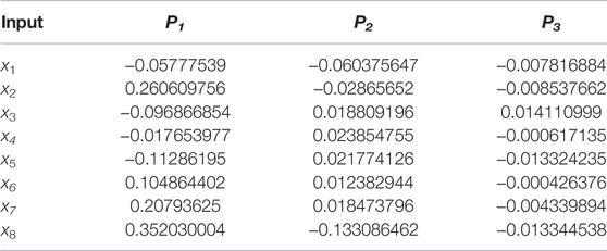
TABLE 3. Parameters of the ith network in autumn prediction result.

According to Eq. 28, the input and output of the B-xNNs consisting of M bootstrap replicate networks can be expressed by the following mathematical relations:

$\overline{f}=\frac{1}{M}{\displaystyle \sum _{i=1}^M{C}_3^{\left(i\right)}{\left(P_3^{\left(i\right)}{X}^T\right)}^3+C_2^{\left(i\right)}{\left(P_2^{\left(i\right)}{X}^T\right)}^2+C_1^{\left(i\right)}\left(P_1^{\left(i\right)}{X}^T\right)+{\mu }^{\left(i\right)}.}(30)$

Obviously, the B-xNNs proposed in this study can directly give the input-output mapping relationship of the prediction model, which can help realize the theoretical analysis between wind speed prediction and input parameters. The output of the probability prediction can be expressed by the mathematical expression:

$\left[L^{\left(\alpha \right)},U^{\left(\alpha \right)}\right]=\left[\overline{f}-F_{\alpha /2},\overline{f}+F_{1-\alpha /2}\right],(31)$

where F_α/2 and F_1-α/2 are determined by the confidence level α setting in the CDF of KED. It should be noted that the process of KDE is data transparent. In other words, the relationship between the probabilistic wind speed prediction results and the output of B-xNNs is very intuitive, whereas the relationship between the wind speed prediction results from B-xNNs and the input parameters is clear. Therefore, the interpretability of the probabilistic proposed method is very easy to understand.

5 Conclusion

In this study, a deterministic approach for wind speed prediction based on B-xNNs is proposed to improve the prediction capability and explain the inherent relationship of neural networks. Then, the proposed approach for deterministic wind speed prediction is extended to a deep framework that can accurately quantify the randomness and uncertainties exhibited in wind speed. The prediction results of the proposed method are extensively compared with two commonly used algorithms, namely, BPNN and LSTM. The prediction results obtained from different seasons show that the proposed probabilistic forecasting method is superior to the two benchmarking algorithms in terms of prediction reliability, prediction accuracy, and interval sharpness. Besides, this study analyzed the interpretability of the probabilistic forecasting model; its novelty is that it reveals how the input variables affect the result of the interval wind speed forecasting model by clear formulation.

In this study, the simulation verification is only carried on one prediction horizon. However, the forecasting reliability may decrease as the number of repeated iterations increases. Therefore, this model may only be applied for short-term wind speed forecasting. In the future, we will further search for the method of long-term forecasting by improving the network structure.

Data Availability Statement

The original contributions presented in the study are included in the article/Supplementary Material. Further inquiries can be directed to the corresponding authors.

Author Contributions

HH contributed to all aspects of this work and conducted data analysis. YH and HW gave useful comments and suggestions to this work and affected the process of the research. All authors reviewed the manuscript.

Funding

This paper has been jointly supported by the National Natural Science Foundation of China (Grant no. 52177102), the Natural Science Foundation of Guangdong Province (Grant no. 2021A1515011685), and the Foundations of Shenzhen Science and Technology Committee (Grant nos. JCYJ20190808143619749 and GJHZ20200731095610032).

Conflict of Interest

The authors declare that the research was conducted in the absence of any commercial or financial relationships that could be construed as a potential conflict of interest.

Publisher’s Note

All claims expressed in this article are solely those of the authors and do not necessarily represent those of their affiliated organizations or those of the publisher, the editors, and the reviewers. Any product that may be evaluated in this article, or claim that may be made by its manufacturer, is not guaranteed or endorsed by the publisher.

References

Anjaiah, K., Dash, P. K., and Sahani, M. (2022). A New Protection Scheme for PV-Wind Based DC-ring Microgrid by Using Modified Multifractal Detrended Fluctuation Analysis. Prot. Control Mod. Power Syst. 7 (8), 8. doi:10.1186/s41601-022-00232-3

CrossRef Full Text | Google Scholar

Aurore, D., Philippe, D., Bastien, A., Jordi, B., Christian, B., and Riwal, P. (2020). Sub-Hourly Forecasting of Wind Speed and Wind Energy. Renew. Energy 145, 2373–2379. doi:10.1016/j.renene.2019.07.161

CrossRef Full Text | Google Scholar

Chen, J., Zeng, G.-Q., Zhou, W., Du, W., and Lu, K.-D. (2018). Wind Speed Forecasting Using Nonlinear-Learning Ensemble of Deep Learning Time Series Prediction and Extremal Optimization. Energy Convers. Manag. 165, 681–695. doi:10.1016/j.enconman.2018.03.098

CrossRef Full Text | Google Scholar

Desai, J. P., and Makwana, V. H. (2021). A Novel Out of Step Relaying Algorithm Based on Wavelet Transform and a Deep Learning Machine Model. Prot. Control Mod. Power Syst. 6 (4), 500–511. doi:10.1186/s41601-021-00221-y

CrossRef Full Text | Google Scholar

Duan, J., Zuo, H., Bai, Y., Duan, J., Chang, M., and Chen, B. (2021). Short-Term Wind Speed Forecasting Using Recurrent Neural Networks with Error Correction. Energy 217, 119397. doi:10.1016/j.energy.2020.119397

CrossRef Full Text | Google Scholar

Efron, B., and Tibshirani, R. J. (1993). An Introduction to the Bootstrap. New York, NY, USA: Chapman & Hall CRC.

Google Scholar

Fu, X. (2022). Statistical Machine Learning Model for Capacitor Planning Considering Uncertainties in Photovoltaic Power. Prot. Control Mod. Power Syst. 7 (5), 5. doi:10.1186/s41601-022-00228-z

CrossRef Full Text | Google Scholar

Guignard, F., Amato, F., and Kanevski, M. (2021). Uncertainty Quantification in Extreme Learning Machine: Analytical Developments, Variance Estimates and Confidence Intervals. Neurocomputing 456, 436–449. doi:10.1016/j.neucom.2021.04.027

CrossRef Full Text | Google Scholar

Haque, A. U., Nehrir, M. H., and Mandal, P. (2014). A Hybrid Intelligent Model for Deterministic and Quantile Regression Approach for Probabilistic Wind Power Forecasting. IEEE Trans. Power Syst. 29 (4), 1663–1672. doi:10.1109/tpwrs.2014.2299801

CrossRef Full Text | Google Scholar

Khodayar, M., Wang, J., and Manthouri, M. (2019). Interval Deep Generative Neural Network for Wind Speed Forecasting. IEEE Trans. Smart Grid 10 (4), 3974–3989. doi:10.1109/tsg.2018.2847223

CrossRef Full Text | Google Scholar

Li, Z., Ye, L., Zhao, Y., Song, X., Teng, J., and Jin, J. (2016). Short-Term Wind Power Prediction Based on Extreme Learning Machine with Error Correction. Prot. Control Mod. Power Syst. 1, 1. doi:10.1186/s41601-016-0016-y

CrossRef Full Text | Google Scholar

Liu, H., Tian, H.-Q., Pan, D.-F., and Li, Y.-F. (2013). Forecasting Models for Wind Speed Using Wavelet, Wavelet Packet, Time Series and Artificial Neural Networks. Appl. Energy 107, 191–208. doi:10.1016/j.apenergy.2013.02.002

CrossRef Full Text | Google Scholar

Long, H., Fu, X., Kong, W., Chen, H., Zhou, Y., and Yang, F. (2022). Key Technologies and Applications of Rural Energy Internet in China. Inf. Process. Agric. Online. doi:10.1016/j.inpa.2022.03.001

CrossRef Full Text | Google Scholar

Madhiarasan, M. (2020). Accurate Prediction of Different Forecast Horizons Wind Speed Using a Recursive Radial Basis Function Neural Network. Prot. Control Mod. Power Syst. 5, 22. doi:10.1186/s41601-020-00166-8

CrossRef Full Text | Google Scholar

Pokhrel, J., and Seo, J. (2021). Statistical Model for Fragility Estimates of Offshore Wind Turbines Subjected to Aero-Hydro Dynamic Loads. Renew. Energy 163, 1495–1507. doi:10.1016/j.renene.2020.10.015

CrossRef Full Text | Google Scholar

Scheu, M. N., Kolios, A., Fischer, T., and Brennan, F. (2017). Influence of Statistical Uncertainty of Component Reliability Estimations on Offshore Wind Farm Availability. Reliab. Eng. Syst. Saf. 168, 28–39. doi:10.1016/j.ress.2017.05.021

CrossRef Full Text | Google Scholar

Tang, G., Wu, Y., Li, C., Wong, P. K., Xiao, Z., and An, X. (2020). A Novel Wind Speed Interval Prediction Based on Error Prediction Method. IEEE Trans. Ind. Inf. 16 (11), 6806–6815. doi:10.1109/tii.2020.2973413

CrossRef Full Text | Google Scholar

Wan, C., Xu, Z., Pinson, P., Dong, Z. Y., and Wong, K. P. (2014). Optimal Prediction Intervals of Wind Power Generation. IEEE Trans. Power Syst. 29 (3), 1166–1174. doi:10.1109/tpwrs.2013.2288100

CrossRef Full Text | Google Scholar

Wan, C., Lin, J., Wang, J., Song, Y., and Dong, Z. Y. (2017). Direct Quantile Regression for Nonparametric Probabilistic Forecasting of Wind Power Generation. IEEE Trans. Power Syst. 32 (4), 2767–2778. doi:10.1109/tpwrs.2016.2625101

CrossRef Full Text | Google Scholar

Wang, H. Z., Wang, G. B., Li, G. Q., Peng, J. C., Liu, Y. T., and Liu, Y. (2016). Deep Belief Network Based Deterministic and Probabilistic Wind Speed Forecasting Approach. Appl. Energy 182, 80–93. doi:10.1016/j.apenergy.2016.08.108

CrossRef Full Text | Google Scholar

Wang, H.-Z., Li, G.-Q., Wang, G.-B., Peng, J.-C., Jiang, H., and Liu, Y.-T. (2017). Deep Learning Based Ensemble Approach for Probabilistic Wind Power Forecasting. Appl. Energy 188, 56–70. doi:10.1016/j.apenergy.2016.11.111

CrossRef Full Text | Google Scholar

Wang, Y., Xie, Z., Hu, Q., and Xiong, S. (2018). Correlation Aware Multi-step Ahead Wind Speed Forecasting with Heteroscedastic Multi-Kernel Learning. Energy Convers. Manag. 163, 384–406. doi:10.1016/j.enconman.2018.02.034

CrossRef Full Text | Google Scholar

Wang, H., Lei, Z., Liu, Y., Peng, J., and Liu, J. (2019a). Echo State Network Based Ensemble Approach for Wind Power Forecasting. Energy Convers. Manag. 201, 112188. doi:10.1016/j.enconman.2019.112188

CrossRef Full Text | Google Scholar

Wang, Y., Shao, X., Liu, C., Cai, G., Kou, L., and Wu, Z. (2019). Analysis of Wind Farm Output Characteristics Based on Descriptive Statistical Analysis and Envelope Domain. Energy 170, 580–591. doi:10.1016/j.energy.2018.12.156

CrossRef Full Text | Google Scholar

Wang, H., Lei, Z., Zhang, X., Zhou, B., and Peng, J. (2019c). A Review of Deep Learning for Renewable Energy Forecasting. Energy Convers. Manag. 198, 111799. doi:10.1016/j.enconman.2019.111799

CrossRef Full Text | Google Scholar

Wang, H., Xue, W., Liu, Y., Peng, J., and Jiang, H. (2020). Probabilistic Wind Power Forecasting Based on Spiking Neural Network. Energy 196, 117072. doi:10.1016/j.energy.2020.117072

CrossRef Full Text | Google Scholar

Wang, H., Cai, R., Zhou, B., Aziz, S., Qin, B., Voropai, N., et al. (2020). Solar Irradiance Forecasting Based on Direct Explainable Neural Network. Energy Convers. Manag. 226, 113487. doi:10.1016/j.enconman.2020.113487

CrossRef Full Text | Google Scholar

Wang, J., Wang, S., Zeng, B., and Lu, H. (2022). A Novel Ensemble Probabilistic Forecasting System for Uncertainty in Wind Speed. Appl. Energy 313, 118796. doi:10.1016/j.apenergy.2022.118796

CrossRef Full Text | Google Scholar

Xin, P., Liu, Y., Yang, N., Song, X., and Huang, Y. (2020). Probability Distribution of Wind Power Volatility Based on the Moving Average Method and Improved Nonparametric Kernel Density Estimation. Glob. Energy Interconnect. 3 (3), 247–258. doi:10.1016/j.gloei.2020.07.006

CrossRef Full Text | Google Scholar

Xu, J., Xiao, Z., Lin, Z., and Li, M. (2021). System Bias Correction of Short-Term Hub-Height Wind Forecasts Using the Kalman Filter. Prot. Control Mod. Power Syst. 6, 37. doi:10.1186/s41601-021-00214-x

CrossRef Full Text | Google Scholar

Xydas, E., Qadrdan, M., Marmaras, C., Cipcigan, L., Jenkins, N., and Ameli, H. (2017). Probabilistic Wind Power Forecasting and its Application in the Scheduling of Gas-Fired Generators. Appl. Energy 192, 382–394. doi:10.1016/j.apenergy.2016.10.019

CrossRef Full Text | Google Scholar

Yang, X., Ma, X., Kang, N., and Maihemuti, M. (2018). Probability Interval Prediction of Wind Power Based on KDE Method with Rough Sets and Weighted Markov Chain. IEEE Access 6, 51556–51565. doi:10.1109/access.2018.2870430

CrossRef Full Text | Google Scholar

Yang, Z., Zhang, A., and Sudjianto, A. (2021). GAMI-Net: An Explainable Neural Network Based on Generalized Additive Models with Structured Interactions. Pattern Recognit. 120, 108192. doi:10.1016/j.patcog.2021.108192

CrossRef Full Text | Google Scholar

Yildiz, C., Acikgoz, H., Korkmaz, D., and Budak, U. (2021). An Improved Residual-Based Convolutional Neural Network for Very Short-Term Wind Power Forecasting. Energy Convers. Manag. 228 (11), 113731. doi:10.1016/j.enconman.2020.113731

CrossRef Full Text | Google Scholar

Zhang, Y., Wang, J., and Luo, X. (2015). Probabilistic Wind Power Forecasting Based on Logarithmic Transformation and Boundary Kernel. Energy Convers. Manag. 96, 440–451. doi:10.1016/j.enconman.2015.03.012

CrossRef Full Text | Google Scholar

Zhao, Y., Ye, L., Li, Z., Song, X., Lang, Y., and Su, J. (2016). A Novel Bidirectional Mechanism Based on Time Series Model for Wind Power Forecasting. Appl. Energy 177, 793–803. doi:10.1016/j.apenergy.2016.03.096

CrossRef Full Text | Google Scholar

Zhao, X., Liu, J., Yu, D., and Chang, J. (2018). One-day-Ahead Probabilistic Wind Speed Forecast Based on Optimized Numerical Weather Prediction Data. Energy Convers. Manag. 164, 560–569. doi:10.1016/j.enconman.2018.03.030

CrossRef Full Text | Google Scholar