Data-Driven Reliability Evaluation of the Integrated Energy System Considering Optimal Service Restoration

The demand for environmental protection and energy utilization transformation has promoted the rapid development of integrated energy systems (IES). Reliability evaluation is a fundamental element in designing IES as it could instruct the planning and operation of IES. This study proposes a novel data-driven reliability improvement and evaluation method considering the three-state reliability model and an optimal service restoration model (OSR). First, a multi-energy flow model is introduced and linearized in order to reduce the computing complexity. Next, a three-state reliability model is developed, considering the transitional process and partial failure mode. Furthermore, an optimal service restoration model is established to determine the best repairment moment for minimizing the load curtailment, and a data-driven reliability evaluation method is developed that integrates OSR and models the stochastic state transition process using the historical measurement data of the smart meters. Finally, the proposed reliability evaluation method is tested on a test IES, and the numerical results validate its effectiveness in evaluating the reliability of IES and improving the overall reliability.

1 Introduction

Concerns over environmental pollution and fossil fuel depletion have been urging us to explore more efficient and low-carbon energy utilization methods (Xu et al., 2020; Zhang et al., 2020; Li P. et al., 2021). The integrated energy system (IES) has received increasing attention (Zhang G. et al., 2021) as it has the merits of improved energy utilization efficiency and low carbon emissions. The IES couples different forms of energy such as electricity, gas, and heat in a synthetic manner and, thus, achieves mutual complementarity and support as well as coordinated optimization of multiple energy scheduling (Zhang Y. et al., 2021). However, the complex composition and structure of the IES also increase the operational complexity remarkably, which exerts significant influence on the energy supplying reliability of IES and poses a great challenge to the widespread application of IES (Li J. et al., 2021). Therefore, it is imperative to investigate advanced reliability evaluation and improvement methods for IES.

The reliability assessment for convention power systems has been extensively investigated(Li, 2014). However, only a few efforts have been devoted to research on IES reliability evaluation and improvement. Basically, establishing the reliability model of system components is the key step for analyzing system operation status and assessing system overall reliability. Zhang et al. (2018) and Yan et al. (2021) used a typical two-state model of components to describe the reliability of IES components and obtain the failure rate of the components based on the statistical results. Bao et al. (2019) developed a multi-state model for gas source, compressor, and gas storage to evaluate the reliability of a natural gas system based on universal generating function. Wang et al. (2013) proposed a state space method based on the probabilistic analysis of the Markov model, which uses a two-state model to analyze the sub-system of different components and then further derives the reliability model of the whole component. In the work of Fu et al. (2018), a data-driven model was established to estimate the probability of incident of an insufficient natural gas supply arising from the uncertainty of weather as well as the impact on the reliability of IES. To sum up, although aforementioned research works have made great progress in the reliability modeling of multi-energy system, they fail to account for the actual operating characteristics, transitional process and heterogeneity of various components.

The reliability evaluation outcome heavily relies on the actual applied evaluation method. Thus, developing an appropriate reliability assessment method could benefit the stakeholders by improving the evaluation accuracy. Up to now, several methods have been proposed by researchers (Shariatkhah et al., 2015; Ansari et al., 2020; Cao et al., 2021; Chi et al., 2021). To name a few, H. Wang. et al. (Cao et al., 2021) proposed a reliability assessment framework combining IES dynamic optimal energy flow and Monte Carlo simulation to identify the overall risk of the multi-energy system. In the work of Shariatkhah et al. (2015), a sequential Monte Carlo method incorporating Markov chains is proposed to assess the energy supply reliability of IES. Chi et al. (2021) evaluated the probability distribution of each functional state of the IES based on machine learning methods and statistical methods. In the work of Ansari et al. (2020), a data-driven method via mixture models and importance sampling is proposed to construct time-dependent probability distributions of wind-integrated systems. However, the aforementioned studies mainly focus on improving the reliability evaluation efficiency without considering the potential attempts like repair scheduling to enhance the overall system reliability and fail to take into account the impact of optimization of system operation on the reliability outcome.

Generally, the influence of component failure can be mitigated by the network reconfiguration and repair scheduling optimization and thus the overall reliability can be improved. In the work of Sultana et al. (2016), a comparative analysis of reliability improvement and power loss reduction of distribution networks was conducted using different network reconfiguration technologies. Basically, the network can be reconfigured and some of the affected load can be transferred without being disturbed. However, the network reconfiguration can only maintain partial load supply and cannot fully alleviate the impact of the failure. In contrast, the system service restoration optimization can be adopted to quickly schedule the repair crews and restore the damaged components in order to minimize the impact of the failure. In the work of Lei et al. (2019), a method of disaster recovery logistics is proposed to optimize service restoration of the distribution network with the scheduling of repair crews and mobile power sources. In the work of Li et al. (2022), a multi-level collaborative optimization model is proposed to integrate the repair unit scheduling and the distribution network restoration. Inspired by these works, the network reconfiguration and service restoration are integrated in the reliability assessment method to improve the overall reliability.

To sum up, most existing works have not considered the influence of partial failure mode and optimization of system operation on the IES reliability outcome. To fill this research gap, this paper proposes an advanced data-driven reliability evaluation and improvement method for IES considering partial failure mode and optimal service restoration. Firstly, a three-state reliability model has been developed for IES to describe the component state transition. Secondly, the influence of the repairment scheduling decision of damaged components is analyzed and an optimal service restoration model is established. Finally, a data-driven reliability evaluation method incorporating the optimal service restoration has been developed. The contributions of this paper are three-fold as follows.

1) A novel three-state reliability model is proposed, including the full-up state, full-down state, derated state and the state transition limits, which can better describe the actual operating states of the components.

2) An optimal service restoration model is established considering the three-state models and repair scheduling decisions. Using the proposed model, the best repairment moment can be autonomously determined so as to minimize the overall load curtailment.

3) By integrating with the optimal service restoration model, a data-driven reliability evaluation method is proposed. Consequently, the overall reliability is enhanced and the accuracy of the evaluation outcome is improved.

The remainder of the paper is organized as follows. Section 1 introduces the energy flow model of IES. Section 2 develops a three-state reliability model for IES components and analyzes the influence of the repair scheduling decision. Section 3 proposes an optimal service restoration model and reliability evaluation method for IES. Section 4 implements the simulations and discusses the numerical results. Finally, Section 5 concludes this paper.

2 Energy Flow Model of the Integrated Energy System

IES integrates the electric power distribution network (DN), natural gas network (NGN), and heat network (HN) through the energy hub. The structure of the heat network is much more complex than the natural gas network and electric power distribution network. Hence, we did not consider the detailed heat network structure for simplicity and concentrated on the main purpose of our research. The structure of IES is illustrated in Figure 1. Substation and distributed generators, e.g., photovoltaic systems (PV) and wind turbines (WT), are the sources of electric energy, while the natural gas is provided by the natural gas sources. The energy hubs are the energy conversion devices that convert one type of energy into another type, consisting of electric boilers (EB), combined heat and power generators (CHP), and gas fired boilers (GB).

FIGURE 1

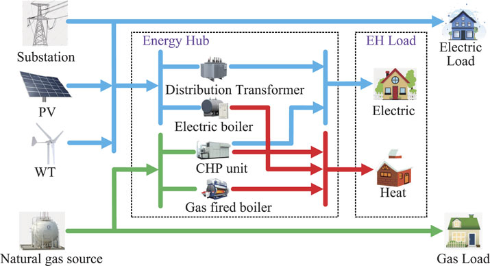
FIGURE 1. Multi-energy flow diagram of IES.

2.1 Electric Power Distribution Network Model

Electric power is delivered through the DN to the end-use customers. Generally, the DN is operated in a radial manner (Zeng et al., 2016) and thus can be represented by a directed tree G = (N_d, N_b), where N_d = 0, 1, … , N denotes the set of buses, and N_b denotes the set of branches. Note that each bus I except the substation bus indexed by 0 has a unique parent bus labeled as Π_i. Each bus i may have several child buses, and the set of child buses of bus i is labeled as C_i. Since each bus except bus 0 has a unique incoming branch, the incoming branch can be labeled with the index of the corresponding bus. Specifically, the branch pointing from a parent bus Π_i to bus i is labeled as i for consistency. Therefore, the set of branches can be expressed as N_b = 1, … , N (Li et al., 2019).

To model the power flow in DN, the linear DistFlow model (Yeh et al., 2012) is adopted as (1) by neglecting the line loss and assuming a relatively flat voltage profile. The applicability of the linear DistFlow model has been validated through its wide applications in resolving practical operational issues in DN, such as voltage violations (Zhu and Liu, 2015) and line overloading (Haque et al., 2020).

$P_i-\sum _{j\in C_i}{P}_j=-p_i\forall i\in N_d,(\mathrm{1a})$

$Q_i-\sum _{j\in C_i}{Q}_j=-q_i\forall i\in N_d,(\mathrm{1b})$

$V_{{\Pi }_i}-V_i=r_i{P}_i+x_i{Q}_i\forall i\in N_b.(\mathrm{1c})$

Eqs. 1a, 1b describe the active and reactive power balance at each bus, where p_i and q_i are the active and reactive power injection at bus i, P_i and Q_i are the active and reactive power on branch i. Eq. 1a shows the voltage drop on branch i, where V_i is the voltage magnitude of bus i, r_i and x_i are the resistance and reactance of branch i.

2.2 Natural Gas Network Model

Natural gas transmission and consumption in steady-state can be described by the energy balance equation as Eq. 2 based on the law of conservation of mass Abeysekera et al. (2016).

${\mathit{A}}_{\mathit{g}}\mathit{f}+{\mathit{L}}_{\mathit{g}}=\mathbf{0},(2)$

where A_g is the NGN node-pipe incidence matrix (Osiadacz, 1987); f is the vector of pipeline flow of NGN; and L_g is the vector of nodal gas load.

As is known, the natural gas pipeline flow rate f_mn is related to the pressure difference between two terminal ends m and n (Abeysekera et al., 2016). Low and medium pressure natural gas networks can be represented by the well-known Lacey’s equation (Abeysekera et al., 2016) as follows:

$|f_{mn}|f_{mn}=32.7184\times 10^{-8}\frac{\left({\pi }_m-{\pi }_n\right)D^5}{f_{r}LS}\forall mn\in N_p,(3)$

where f_mn is the gas flow rate of the pipeline mn. When f_mn is positive, the gas flow is from node m to node n; otherwise, it is from node n to node m. π_m and π_n are the air pressure at nodes m and n, respectively; D is the diameter of the pipeline; f_r is the friction coefficient of the pipeline wall; L is the length of the pipeline; S is the specific gravity of the gas; N_p is the set of NGN pipelines. Note that for a given natural gas network, the parameters D, f_r, S, and N_p are known.

It can be observed from Eq. 3 that the Lacey formula 3 is nonlinear. To reduce computational complexity, it is linearized using the piece-wise linearization technique (Correa-Posada and Sanchez-Martin, 2014). The nonlinear term |f_mn|f_mn in Eq. 3 is generalized as h(x) = |x|x and f_mn is denoted by a general notation x. Since the gas flow rate f_mn is constrained by the pipeline transmission capacity, without loss of generality, x is defined within the interval [A, B], where A and B are associated with the transmission capacity. The operating interval [A, B] is divided into Z – 1 segments and the value of h(x) at each segment is represented by the line segment between h(X_z) and h(X_z+1) as illustrated in Figure 2, where X_z and X_z+1 are the two terminal points of the z-th segment. Hence, the piece-wise linearized approximation of h(x) can be represented by the following equations:

$h\left(x\right)\approx h\left(X_1\right)+\sum _{z=1}^{Z-1}\left[h\left(X_{z+1}\right)-h\left(X_z\right)\right]{\delta }_z,(\mathrm{4a})$

$x=X_1+\sum _{z=1}^{Z-1}\left(X_{z+1}-X_z\right){\delta }_z,(\mathrm{4b})$

${\delta }_{z+1}\le {\sigma }_z\le {\delta }_{z}z\in \left\{1,\dots ,Z-2\right\},(\mathrm{4c})$

$0\le {\delta }_z\le 1z\in \left\{1,\dots ,Z-1\right\},(\mathrm{4d})$

where δ_z is a continuous variable that represents the portion of the z-th segment; σ_z is an auxiliary binary variable that indicates whether x lies on the right-side of the z-th segment. Specifically, if X_z < x ≤ X_z+1, then σ_t = 1 for all t ≤ z and σ_t = 0 for all t > z.

FIGURE 2

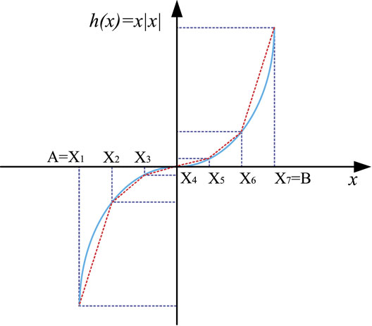
FIGURE 2. Graphical illustration of the piece-wise linearization of function h(x).

2.3 Energy Hub Model

The EH interconnects different energy systems and thus could provide a certain degree of flexibility for the coordination of multi-energy systems (Lei et al., 2018). In this paper, two types of EH structures are used to model the energy conversion within the multi-energy system, which is demonstrated in Figure 3. Type-A EH consists of a distribution transformer (DT), CHP, and GB, and type-B EH is composed of DT, CHP, and EB. For both types of EH, the input energy consists of electricity and gas, while the output energy consists of electricity and heat. The energy conversion in EHs can be described by the following equation:

$\left[\begin{array}{c}\hfill L^{ehe}\hfill \\ \hfill L^{ehh}\hfill \end{array}\right]=\left[\begin{array}{cc}\hfill \left(1-v_e\right){\eta }^{DT}\hfill & \hfill \left(1-v_g\right){\eta }_{ge}^{CHP}\hfill \\ \hfill v_e{\eta }^{EB}\hfill & \hfill \left(1-v_g\right){\eta }_{gh}^{CHP}+v_g{\eta }^{GB}\hfill \end{array}\right]\left[\begin{array}{c}\hfill P^{ehe}\hfill \\ \hfill P^{ehg}\hfill \end{array}\right],(5)$

where the superscripts ehe, ehg, and ehh denote electricity, natural gas, and heat, respectively; P and L are input and output vectors, respectively; P^ehg = F^ehgGHV is the natural gas flow injected into EH, and GHV is the natural gas high calorific value; ${\eta }_{ge}^{CHP}$ and ${\eta }_{gh}^{CHP}$ are the efficiencies of CHP for converting natural gas energy into electric energy and heat energy, respectively; η^DT is the efficiency of the distribution transformer; η^GB and η^EB are the efficiency of the gas fired boiler and electrical boiler, respectively; v_g and v_e represent the proportion of natural gas feeding into GB and the proportion of electric energy feeding into EB, respectively. The values of v_g and v_e lie between 0 and 1. For type-A EH, v_e = 0, and for type-B EH, v_g = 0.

FIGURE 3

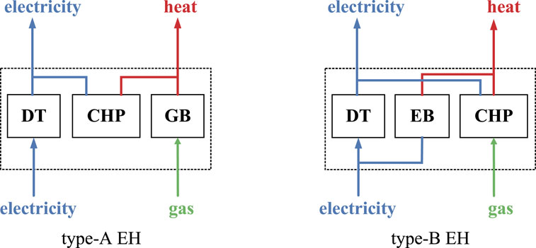
FIGURE 3. Two typical types of energy hub.

It can be observed from Eq. 5 that the formula 5 is nonlinear. To reduce computational complexity, the auxiliary variables are introduced to replace the nonlinear term with an independent variable. Specifically, we introduce P^DT, P^EB, $P_{ge}^{CHP}$, $P_{gh}^{CHP}$ and P^GB to represent (1 − v_e)η^DTP^ehe, v_eη^EBP^ehe, $(1-v_g){\eta }_{ge}^{CHP}{P}^{ehg}$, $(1-v_g){\eta }_{gh}^{CHP}{P}^{ehg}$ and v_gη^GBP^ehg, respectively. Therefore, formula 5 can be reformulated as the following linearized equations:

$L^{ehe}=P^{DT}+P_{ge}^{CHP},(\mathrm{6a})$

$L^{ehh}=P^{EB}+P_{gh}^{CHP}+P^{GB},(\mathrm{6b})$

$P^{ehe}=P^{DT}/{\eta }^{DT}+P^{EB}/{\eta }^{EB},(\mathrm{6c})$

$P^{ehg}=P_{ge}^{CHP}/{\eta }_{ge}^{CHP}+P^{GB}/{\eta }^{GB},(\mathrm{6d})$

where P^DT is the active power output of the distribution transformer; $P_{ge}^{CHP}$ and $P_{gh}^{CHP}$ are the active power output of CHP for converting natural gas energy into electric energy and heat energy, respectively; P^EB and P^GB are the active power output of the gas fired boiler and electrical boiler, respectively. Furthermore, $P_{gh}^{CHP}$ is equal to $({\eta }_{gh}^{CHP}/{\eta }_{ge}^{CHP})P_{ge}^{CHP}$.

3 Reliability Model of the Integrated Energy System

As the IES integrates DN and NGN, its reliability level is influenced jointly by the operating state of DN and NGN as well as the healthy state of the coupling equipment like EHs. Since the failure of the coupling equipment could threaten the reliable operation of both the electric power network and the natural gas network, more efforts should be devoted to the investigation of the impact of the coupling equipment on the overall reliability of the entire IES.

3.1 Reliability Model of the System

Conventionally, the states of all components are represented by the two-state model in evaluating the reliability of the whole system. However, it fails to account for the actual operating characteristics, transitional processes, and heterogeneity of various components.

Generally, it is sufficient to use the two-state model to represent most components. For instance, DN branches and NGN pipelines are either in a full-up state or in a full-down state. For some coupling equipment and energy sources, the derated state, aks. partial failure mode, is commonly observed in practice, and thus it is necessary to take the derated state into account as it could exert a great influence on the overall reliability assessment. The partial failure mode could last for a long period and could eventually lead to the full-down state if not repaired, thereby causing significant economic losses. The partial failure mode could also be restored to the full-up state after repair. Therefore, this paper proposes a novel three-state model that integrates full-up state, full-down state, and derated state as illustrated in Figure 4.

FIGURE 4

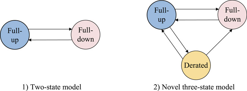
FIGURE 4. State space diagram of the component.

As previously discussed, the states of DN branches and NGN pipelines can be described by the two-state mode as

Eq. 7a, and the states of other components like substation, natural gas source and coupling devices including DT, CHP, GB, EB are represented by the three-state model as Eq. 7b.

$u_{d,t}=\left\{\begin{array}{cc}\hfill 1& \text{if}full-up\hfill \\ \hfill 0& \text{if}full-down\hfill \end{array}\right.(\mathrm{7a})$

$u_{m,t}=\left\{\begin{array}{cc}\hfill 1& \text{if}full-up\hfill \\ \hfill \xi & \text{if}derated\hfill \\ \hfill 0& \text{if}full-down\hfill \end{array}\right.(\mathrm{7b})$

where u_d,t denotes the state of the component d at time t described by the two-state model, u_m,t denotes the state of the component m at time t described by the three-state model, and ξ represents the ratio of the actual available capacity of the component m in derated state to rated capacity in full-up state. ξ can be any value between 0 and 1.

3.2 Influence of Repair Scheduling Decision

After a component damage event, the system operator needs to perform the damage assessment before mobilizing the repair crew to repair the damaged components. The reliability assessment is highly related to the repairment scheduling decision (Arif et al., 2018).

To mitigate the impact of damaged components, the system operator should determine the repair schedule decision by either mobilizing the repair crew to immediately repair the damaged components or delaying the repair for a certain period. If the damaged component is in a full-down state, the repair should be immediately performed so as to minimize load curtailment. If the damaged component is in a derated state, the system operator will invoke the optimal service restoration process (which is introduced in the following section) to determine the best moment for the repair taking into account the system operating condition and load predication profiles in order to achieve the minimal load curtailment.

The initial state of the component m is denoted by u_m,0 and is known to the system operator. It is assumed that if u_m,0 = 1, then the state of the component m is maintained as healthy for the entire assessment horizon, e.g., one week. Thus, the initial state of the component decides whether it needs to be repaired or not, which can be represented as follows:

${\alpha }_m=\left\{\begin{array}{cc}\hfill 1& \text{if\hspace{0.17em}}{u}_{m,t}=0\text{\hspace{0.17em}or\hspace{0.17em}}\xi \hfill \\ \hfill 0& \text{if\hspace{0.17em}}{u}_{m,t}=1\hfill \end{array}\right.(\mathrm{8a})$

${\beta }_m=\left\{\begin{array}{cc}\hfill 1& \text{if\hspace{0.17em}}{u}_{m,t}=\xi \hfill \\ \hfill 0& \text{if\hspace{0.17em}}{u}_{m,t}=0\text{\hspace{0.17em}or\hspace{0.17em}}1\hfill \end{array}\right.(\mathrm{8b})$

where α_m is the indicator that indicates whether the component m needs to be repaired or not. Specifically, if initially the component m is in a full-down or derated state, then it needs to be repaired and α_m is set as 1. β_m is the indicator indicating whether the repair of damaged component m could be delayed or not. If the damaged component is in a derated state, then it does not need to be repaired immediately.

Let T denote the reliability assessment horizon for the IES, which is divided into T time intervals with the duration of each time interval being 1 h. Two binary variables y_m,t and d_m,t are introduced to indicate the repair start time interval and completion time interval. Particularly, $y_{m,t_1}=1$ and $d_{m,t_2}=1$ represent the repair of the damaged component m is started at time interval t₁ and is completed at time interval t₂, respectively. For example, if the repairment of the component m starts at t = 1 and is restored at t = 3, then y_m = {0, 1, 0, 0, … , 0}, d_m = {0, 0, 0, 1, … , 0}; if the component m does not need to be repaired, then y_m = d_m = {0, 0, 0, 0, … , 0}. Constraint Eq. 9b is enforced to guarantee only one of the y_m,t and d_m,t will be set as 1 over the entire horizon if the component m is damaged.

$y_{m,t},d_{m,t}\in \left\{\mathrm{0,1}\right\}\forall m\in N_m,(\mathrm{9a})$

$\sum _{t=1}^T{y}_{m,t}=\sum _{t=1}^T{d}_{m,t}={\alpha }_m\forall m\in N_m,(\mathrm{9b})$

where N_m is a set of the coupling equipment and energy sources in IES. With the binary variables y_m,t and d_m,t, the repair start time and completion time can be represented by ∑_tty_m,t and ∑_ttd_m,t, respectively.

It is required that the derated component should be repaired before reaching the maximum allowed operating time T_df,m as described by Eq. 10a since otherwise the derated component may further be damaged to the full-down state. Eqs. 10b, 10c illustrate the relationship between the repair start time interval ∑_tty_m,t and the completion time interval ∑_ttd_m,t. Specifically, if the component m is in a full-down state, its repairment completion time interval is equal to the round up of the repairment start time interval plus the required repairment time T_fn,m; if the component m is in a derated state, its repairment completion time interval is equal to the round up of the repairment start time plus the required repairment time T_dn,m.

$\sum _{t=1}^{T}t{y}_{m,t}\le T_{df,m}{\beta }_m\forall m\in N_m,(\mathrm{10a})$

$\sum _{t=1}^{T}t{d}_{m,t}\ge \sum _{t=1}^{T}t{y}_{m,t}+T_{fn,m}{\alpha }_m+\left(T_{dn,m}-T_{fn,m}\right){\beta }_m\forall m\in N_m,(\mathrm{10b})$

$\sum _{t=1}^{T}t{d}_{m,t}\le \sum _{t=1}^{T}t{y}_{m,t}+T_{fn,m}{\alpha }_m+\left(T_{dn,m}-T_{fn,m}\right){\beta }_m+1-ϵ\forall m\in N_m,(\mathrm{10c})$

where ϵ is a very small number.

The component state u_m,t can also be viewed as the availability of the component m. In particular, when u_m,t = 0 either in full-down state or during the repairment, component m is unavailable at time interval t; when u_m,t = 1 either the initial state is full-up or it has been repaired, component m is fully available at time interval t; when u_m,t is equal to other value between 0 and 1, component m is partially available. For instance, if u_m,t = 0.5, only half of the rated capacity of the component m can be used. To derive the logical relationship between u_m,t and d_m,t, we further introduce an auxiliary binary variable χ_m,t which indicates the repairment state and can be represented by Eq. 11a. Then, u_m,t can be expressed as a function of χ_m,t, d_m,τ and u_m,0 as Eq. 11b.

${\chi }_{m,t}=\sum _{\tau =1}^t\left(y_{m,\tau }-d_{m,\tau }\right)\forall m\in N_m,(\mathrm{11a})$

$u_{m,t}=u_{m,0}\left(1-{\chi }_{m,t}\right)+\left(1-u_{m,0}\right)\sum _{\tau =1}^t{d}_{m,\tau }\forall m\in N_m.(\mathrm{11b})$

The following three examples with different initial states are used to illustrate the influence of the repairment scheduling decision on the state/availability of each component m represented by Eq. 11b. Suppose the required repair times T_fn,m and T_dn,m are 3 h and 2 h, respectively, and the maximum allowed operating time T_df,m for the derated state is 3 h. If initially the component m is in full-up state, it will be maintained in a full-up state for the entire assessment horizon t = {0, 1, 2, 3, 4, 5}. Hence, it does not need to be repaired. Consequently, we have y_m = {0, 0, 0, 0, 0, 0} and d_m = {0, 0, 0, 0, 0, 0, 0}. Then, according to (11a) and (11b), we have χ_m = {0, 0, 0, 0, 0, 0} and u_m = {1, 1, 1, 1, 1, 1, 1} as illustrated by Figure 5A.

FIGURE 5

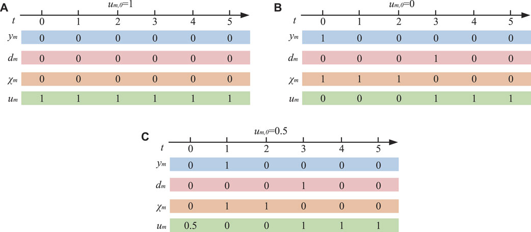
FIGURE 5. Illustration of the relationship between y_m, f_m and χ_m, u_m when u_m,0 is different values, (A) is u_m,0 = 1, (B) is u_m,0 = 0, (C) is u_m,0 = 0.5.

If initially the component m is in full-down state, the repair should be started immediately at time t = 0 and is completed at time t = 3 so as to minimize the load curtailment. After that, it will return to the full-up state for the remainder of the assessment horizon. Consequently, we have y_m = {1, 0, 0, 0, 0, 0} and d_m = {0, 0, 0, 1, 0, 0, 0}. Then, according to Eqs 11a, 11b, we have χ_m = {1, 1, 1, 0, 0, 0} and u_m = {0, 0, 0, 1, 1, 1, 1} as illustrated by Figure 5B.

If initially the component m is in a derated state (for instance, u_m,0 = 0.5), the optimal service restoration process will be invoked (which is introduced in the following section) to determine the best moment of repairment in order to achieve the minimal load curtailment. The component m will remain in the derated operating state until the repairment start time, i.e., t = 1 in this example. When the repairment of the component m is completed (i.e., t = 3 in this example), it will return to the full-up state for the remainder of the assessment horizon. Hence, we have y_m = {0, 1, 0, 0, 0, 0} and d_m = {0, 0, 0, 1, 0, 0}. Then, according to (11a) and Eq. 11b, we have χ_m = {0, 1, 1, 0, 0, 0} and u_m = {0.5, 0, 0, 1, 1, 1, 1} as illustrated by Figure 5C.

4 Reliability Improvement and Evaluation With Optimal Service Restoration

4.1 Optimal Service Restoration Model

In order to improve the IES overall reliability, a novel optimal service restoration (OSR) model is proposed, considering the multi-state mode of various equipment. The optimal repair scheduling decision in Section 2.2 is obtained by solving the OSR model to mitigate the adverse impact caused by the failure of IES components.

4.1.1 Objective Function

The objective of the OSR model is to minimize the overall load curtailment cost, including electric load curtailment cost in DN, natural gas load curtailment cost in NGN, as well as electric load curtailment cost and thermal load curtailment cost in EHs, which is formulated as follows:

$\mathrm{m}\mathrm{i}\mathrm{n}\mathrm{f}=\sum _{t=1}^T\left[\sum _{i=0}^{N_d}{\lambda }_{e,i}\mathrm{\Delta }{P}_{i,t}^D+\sum _{n=1}^{N_n}{\lambda }_{g,n}\mathrm{\Delta }{F}_{n,t}^D+\sum _{k=1}^{N_{eh}}\left({\lambda }_{e,k}\mathrm{\Delta }{L}_{k,t}^{ehe}+{\lambda }_{h,k}\mathrm{\Delta }{L}_{k,t}^{ehh}\right)\right],(12)$

where the first term is the electric load curtailment cost in DN, the second term is the natural gas load curtailment cost in NGN, and the last two terms are the electric load curtailment cost and thermal load curtailment cost in EHs, respectively; $\mathrm{\Delta }{P}_{i,t}^D$, $\mathrm{\Delta }{F}_{n,t}^D$, $\mathrm{\Delta }{L}_{k,t}^{ehe}$, $\mathrm{\Delta }{L}_{k,t}^{ehh}$ are the electric load curtailment of DN bus i at time t, the natural gas load curtailment of NGN node n at time t, the electric load curtailment of EH k at time t, and the thermal load curtailment of EH k at time t, respectively; λ_e,i, λ_g,n, λ_e,k, and λ_h,k are the corresponding unit curtailment costs; N_n and N_eh are the total numbers of NGN nodes and EHs, respectively.

4.1.2 Network Reconfiguration

When the IES is inflicted with damage, the networks can be reconfigured such that the fault can be isolated and the load in the unfaulted region can be transferred and supplied by other power sources. As a result, the load curtailment can be reduced and the overall reliability can be enhanced.

Practically, not every DN branch and NGN pipeline is switchable. In fact, several buses/nodes are interconnected by the non-switchable branches/pipelines. Hence, these buses/nodes can be clustered as a bus/node block, and the bus/node blocks are interconnected by the switchable branches/pipelines. Therefore, to reduce the computational complexity, a virtual power/gas flow model is adopted, taking into account the bus/node blocks (Arif et al., 2019). To this end, the virtual load is introduced for each DN bus block and NGN node block, which is essentially a binary variable indicating the energization status of the DN bus block and NGN node block. In DN, each bus block can only be energized by the black-start power sources, e.g., substation and CHP, through a connected energization path. Thus, for an isolated network without black-start power sources, all internal nodes are de-energized and all internal loads are un-served. Likewise, each NGN node block can only be energized by the natural gas sources through a connected energization path. The proposed virtual power/gas flow model is introduced as follows:

$g_{i,t}+\sum _{\left(i,k\right)\in L^R}{v}_{ik,t}=X_{i,t}+\sum _{\left(k,j\right)\in L^R}{v}_{kj,t}\forall i,t,(\mathrm{13a})$

$g_{I,t}=0\forall i\in {\mathrm{\Omega }}_B\backslash \left\{{\mathrm{\Omega }}_{NS}\right\},(\mathrm{13b})$

$-u_{ik,t}M\le v_{ik,t}\le u_{ik,t}M\forall \left(i,k\right)\in L^R,t.(\mathrm{13c})$

Constraint Eq. 13a represents the virtual power flow balance for each DN bus block/NGN node block, where g_i,t is the output of a power/gas source in block I at time t, v_ik,t is the virtual power/gas flow transferred from block i to block k, L^R is the set of the switchable branches/pipelines, and X_i,t is the energization status associated with the virtual load of block i. Constraint Eq. 13b requires the outputs of the non-black-start power/gas sources to be 0, where Ω_B is the set of the energy sources, Ω_NS is the set of the black-start power sources in DN, and is the set of the natural gas sources in NGN. Constraint Eq. 13c imposes the capacity limits on the switchable branches/pipelines, where u_ik,t is the availability of the switchable branch/pipeline connecting blocks i and k, M is a very large number. If the virtual load can be served by the energy sources, then X_i = 1 (i.e., block i is energized); otherwise, X_i = 0 (i.e., block i de-energized).

4.1.3 Nodal Power Balance

The nodal power balance, gas balance, and EH load balance equation can be formulated as follows:

$p_{i,t}=P_{i,t}^{TS}+P_{i,t}^{wt}+P_{i,t}^{pv}-P_{i,t}^{ehe}-\mathrm{\Delta }{P}_{i,t}^{wt}-\mathrm{\Delta }{P}_{i,t}^{pv}-\left(P_{i,t}^D-\mathrm{\Delta }{P}_{i,t}^D\right)\forall i\in N_d,(\mathrm{14a})$

$q_{i,t}=Q_{i,t}^{TS}+Q_{i,t}^{wt}+Q_{i,t}^{pv}+Q_{i,t}^C-\left(Q_{i,t}^D-\mathrm{\Delta }{P}_{i,t}^D\left(Q_{i,t}^D/P_{i,t}^D\right)\right)\forall i\in N_d,(\mathrm{14b})$

$f_{n,t}=F_{\text{n},t}^{\mathrm{G}\mathrm{S}}-F_{n,t}^{ehg}-\left(F_{n,t}^D-\mathrm{\Delta }{F}_{n,t}^D\right)\forall n\in N_n,(\mathrm{14c})$

$L_{k,t}^{ehe}=P_{k,t}^{DT}+P_{ge,k,t}^{CHP}+\mathrm{\Delta }{L}_{k,t}^{ehe}\forall k\in N_{eh},(\mathrm{14d})$

$L_{k,t}^{ehh}=P_{k,t}^{EB}+P_{gh,k,t}^{CHP}+P_{k,t}^{GB}+\mathrm{\Delta }{L}_{k,t}^{ehh}\forall k\in N_{eh}.(14e)$

Constraint Eq. 14a shows the composition of the nodal active power injection, where $P_{i,t}^{TS}$, $P_{i,t}^{wt}$, $P_{i,t}^{pv}$, $P_{i,t}^{ehe}$, $P_{i,t}^D$ are the active power of subtation, WT, PV, EH and load at bus i at time t, respectively; $\mathrm{\Delta }{P}_{i,t}^{wt}$, $\mathrm{\Delta }{P}_{i,t}^{pv}$ are the amount of curtailed wind power and solar power at bus i at time t, respectively. Constraint Eq. 14b illustrates the composition of the nodal reactive power injection, where $Q_{i,t}^{TS}$, $Q_{i,t}^{wt}$, $Q_{i,t}^{pv}$, $Q_{i,t}^C$, $Q_{i,t}^D$ are the reactive power of subtation, WT, PV, compensation devices and load at bus i at time t, respectively. Note that the nodal reactive power load is curtailed proportionally to the nodal active power curtailment. Constraint Eq. 14c reveals that the nodal net gas injection f_n,t at node i is equal to the gas injection $F_{n,t}^{GS}$ by the gas source minus the gas consumption $F_{n,t}^{ehg}$ by the EH and nodal gas load $(F_{n,t}^D-\mathrm{\Delta }{F}_{n,t}^D)$, where $F_{n,t}^D$ is the required nodal gas load and $\mathrm{\Delta }{F}_{n,t}^D$ is the curtailed nodal gas load. Constraints Eqs 14d, 14e are the electric power balance and thermal energy balance in EHs, respectively.

4.1.4 Operational Security Constraints

Three categories of operational security constraints are considered as follows:

1. Operational limits for load curtailment

2. Operational limits for various devices include WT, PV, CHP, DT, GB, and EB

3. Network operational security constraints, including bus voltage limits, node gas pressure limits, branch flow limits, and pipeline flow limits

The abovementioned three categories of constraints can be generalized as the following two mathematical inequalities.

$\mathrm{\Delta }{L}^{\min }\le \mathrm{\Delta }L\le \mathrm{\Delta }{L}^{\max },(\mathrm{15a})$

$u_{w,t}{W}^{\min }\le W\le u_{w,t}{W}^{\max },(\mathrm{15b})$

where $\mathrm{\Delta }L={[\mathrm{\Delta }{P}_{I,t}^D,\mathrm{\Delta }{F}_{n,t}^D,\mathrm{\Delta }{L}_{k,t}^{ehe},\mathrm{\Delta }{L}_{k,t}^{ehh}]}^{\text{T}}$; ΔL^max and ΔL^min denote the upper and lower limits of ΔL, respectively. $\mathrm{W}=[P_{i,t}^{TS},P_{i,t}^{wt},P_{i,t}^{pv},\mathrm{\Delta }{P}_{i,t}^{wt},\mathrm{\Delta }{P}_{i,t}^{pv},Q_{i,t}^{TS},Q_{i,t}^{wt},Q_{i,t}^{pv},Q_{i,t}^C,F_{n,t}^{GS},P_{ge,k,t}^{CHP},P_{gh,k,t}^{CHP},P_{k,t}^{DT},$$P_{k,t}^{GB},P_{k,t}^{EB},V_{i,t},{\pi }_{n,t},T{l}_{i,t},P{l}_{n,t}{]}^T$. u_w,t denotes the state of the component z at time t. W^max and W^min denote the upper and lower limits of W, respectively. Here, $P_{ge,k,t}^{CHP}$, $P_{gh,k,t}^{CHP}$ are the active power output of the heat production and electricity production of CHP, respectively; $P_{k,t}^{DT}$, $P_{k,t}^{GB}$, $P_{k,t}^{EB}$ are the active power output of DT, GB, EB in EH, respectively. V_i,t, π_n,t are bus voltage in DN and node pressure in NGN, respectively. Tl_i,t, Pl_n,t are the capacity of branches in DN and pipelines in NGN, respectively. For example, the bus voltage V_i,t in DN should be within the scope of the up limit V^max and down limit V^min when it is energized. When it is not energized, it is 0.

4.2 Data-Driven Reliability Evaluation Process

Based on the proposed optimal service restoration model, we developed a data-driven reliability evaluation method for the IES that integrates OSR and models the stochastic state transition process using the historical measurement data of the smart meters, whose flowchart is demonstrated in Figure 6.

FIGURE 6

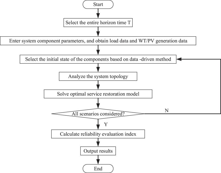
FIGURE 6. Reliability evaluation flowchart of IES.

The proposed reliability evaluation of the IES consists of eight steps illustrated as follows:

Step(B1). We select the reliability assessment horizon T, which is greater than the maximum restoration time of each component.

Step(B2). We enter IES component data and obtain the load, WT, and PV prediction data for the entire horizon T.

Step(B3). The historical measurement data of the smart meters is used to model the state transition probability of each component. Then, we use the Monte Carlo simulation method to get the initial state of the IES components according to the state transition probability distribution.

Step(B4). We analyze DN and NSN topology.

Step(B5). We solve the optimal service restoration model.

Step(B6). We check if all scenarios are considered. If so, we move to Step(B7); otherwise, we go back to Step(B3).

Step(B7). We calculate reliability evaluation indices. The IES reliability evaluation indices used in the paper mainly include the expected electricity not supply EENS, the expected gas not supply EGNS, and the expected heat not supply EHNS. Their calculation formulas are presented as follows:

$EENS=\sum _{X\in E}P\left(X\right)\sum _{t=1}^T\left[\sum _{i=1}^{N_d}\mathrm{\Delta }{P}_{i,t}^D+\sum _{k=1}^{N_{eh}}\mathrm{\Delta }{L}_{k,t}^{ehe}\right],(\mathrm{16a})$

$EGNS=\sum _{X\in G}P\left(X\right)\sum _{t=1}^T\sum _{n=1}^{N_n}\mathrm{\Delta }{F}_{n,t}^D,(\mathrm{16b})$

$EHNS=\sum _{X\in H}P\left(X\right)\sum _{t=1}^T\sum _{k=1}^{N_{eh}}\mathrm{\Delta }{L}_{k,t}^{ehh},(\mathrm{16c})$

where P(X) is the probability of the scenario X.

Step(B8) Output results.

5 Numerical Results

In order to verify the effectiveness of the proposed optimal service restoration model and the proposed reliability evaluation method, case studies on a test IES are carried out on the platform of MATLAB using CPLEX as the MILP solver.

5.1 Test System Specification

The test IES is composed of the modified IEEE 33-node distribution network (Group, 2010), the 11-node natural gas network (Abeysekera et al., 2016) and two EHs, as demonstrated by Figure 7, where EH1 is a type-A EH and EH2 is a type-B EH.

FIGURE 7

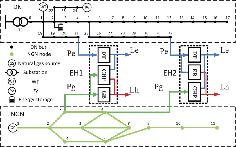
FIGURE 7. Topology of the test IES.

The base voltage of the IEEE 33-node DN is 12.66 kV, and the voltages in the case studies are expressed in per-unit value. The parameter of the derated state ξ is assumed to be 0.5. The upper and lower limits for the nodal voltage magnitude are 0.95 and 1.05, respectively. The maximum and minimum values of nodal pressure in NGN are 75 mbar and 22.5 mbar, respectively. The capacity of the pipeline is 1600 m³/h. The parameters related to the coupling equipment and energy sources in IES are shown in Table 1, and the required repair times for the damaged coupling equipment and energy sources are summarized in Table 2. The assessment horizon of 1 week is considered and the weekly profiles of electric load, gas load, and thermal load are demonstrated in Figure 8, where the peak electric load of DN and NGN can be found in (Group, 2010) and (Abeysekera et al., 2016), respectively. In addition, the peak electric load and heat load in EH are 600 kW and 600 kW, respectively. Besides, the unit cost for electric load curtailment, gas load curtailment, and thermal load curtailment are assumed as 10$, 98$ and 10$, respectively.

TABLE 1

TABLE 1. Parameters of IES components.

TABLE 2

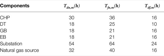
TABLE 2. Reliability parameters of IES components.

FIGURE 8

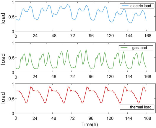
FIGURE 8. Weekly variation profiles of electric/gas/thermal load.

5.2 Effectiveness of the Proposed Three-State Model

In this subsection, the effectiveness of the proposed novel three-state model considering partial failure mode is verified.

Table 3 lists the load curtailments in IES due to the damages occurring to the coupling equipment and energy sources using two different reliability models. As shown in the table, the load curtailment from the two-state model without considering the derated state is much greater than the load curtailment from the proposed three-state model considering the partial failure mode, which validates the effectiveness of the proposed three-state model. The reason is that when a component is in a derated state, it can still be operated for a certain period so that the repair can be delayed to the moment when the net load is relatively low. Therefore, the proposed three-state model outperforms the conventional two-state model, as the proposed three-state model can describe the states of components more accurately.

TABLE 3

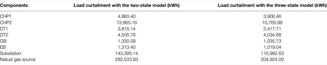
TABLE 3. Performance comparision between the two-state model and the proposed three-state model.

5.3 Effectiveness of the Optimal Service Restoration Model

To demonstrate the merits of the proposed optimal service restoration (OSR) model, its performance is compared with a benchmark approach without considering OSR, denoted as NOSR, for the damages that occurred to different types of components.

Table 4 summarizes the load curtailments in IES due to the derated or full-down states of the coupling equipment and energy sources using the proposed OSR model and the benchmark approach to NOSR. As shown in the table, when the coupling equipment and energy sources are in a full-down state, the amount of load curtailments with the OSR model is the same as that with NOSR. The reason is that when a component is in a full-down state, it should be repaired immediately in order to minimize the load curtailment. When the coupling equipment and energy sources are in derated state, the amount of load curtailments with OSR model is reduced substantially compared to the load curtailments with NOSR since the repairment of the derated component is delayed to the best moment in term of overall load curtailment using the proposed OSR model. Therefore, the proposed OSR model is effective in reducing load curtailment caused by the damage of the key components in IES.

TABLE 4

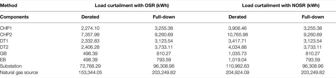
TABLE 4. Comparison of overal load curtailment under different methods.

Figure 9 depicts the load curtailment due to the derated coupling equipment using the proposed OSR method and the NOSR method. It can be observed from the figure that when the coupling equipment is derated, it mainly leads to electric load curtailment and thermal load curtailment within the EH and has little effect on DN and NGN. Besides, the proposed OSR model could significantly lower the overall load curtailment caused by the partial failure of CHP, DT, GB, and EB. Figure 10 shows the load curtailment due to the derated state of the energy sources in IES using the proposed OSR method and the NOSR method. We can see from the figure that when the energy sources are partially damaged, it leads to a large amount of load curtailment in IES and its impact on EH is also considerable. When the substation is partially damaged, it mainly affects the distribution network load and EH electric load supply, and when the natural gas source is partially damaged, it mainly influences the natural gas load and EH thermal load supply. When the OSR method is applied, the load curtailment is substantially lessened. Therefore, the proposed OSR method is more favorable than the benchmark approach NOSR in reducing the load curtailment due to the partial failure of key components.

FIGURE 9

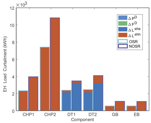
FIGURE 9. Load curtailment due to the derated EH equipment using different methods.

FIGURE 10

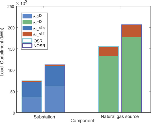
FIGURE 10. Load curtailment due to the derated energy sources using different methods.

Table 5 lists the reliability evaluation indices of the test IES with and without the optimal service restoration model considering the fault scenarios of coupling equipment and energy sources. In each scenario, only one fault is occurred to the aforementioned components, either the full-down failure of derated partial failure. We did not consider the possibility of multiple faults occurring simultaneously on different components as the probability of this scenario is relatively low.

TABLE 5

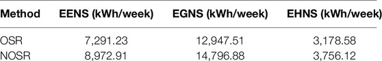
TABLE 5. Reliability evaluation indices using different methods.

From Table 5, it can be seen that the reliability index EGNS is larger than EENS, and EENS is greater than EHNS. Because in the test system, there is only one natural gas source. When the natural gas source fails down, all gas loads are curtailed, which leads to the high value of EGNS. In contrast, the electric loads are served by the substation, PV, WT, and CHP. Thus, even if the substation is out of work, some electric loads can still be served by other power sources. The overall thermal load level is much smaller than the electric load level and gas load level, which results in a lower value of EHNS. Besides, all reliability assessment indices EENS, EGNS, and EHNS are substantially lowered when the OSR model is adopted, which further verifies the effectiveness of the proposed optimal service restoration model in improving the overall reliability of IES.

6 Conclusion

This paper develops a novel reliability improvement and evaluation method by integrating the three-state reliability model and the optimal service restoration model. First, the multi-energy flow model is introduced and linearized to reduce computational complexity. Then, a three-state model is proposed, taking into account the partial failure mode of the IES components based on the conventional two-state model. Furthermore, an innovative optimal service restoration model is developed to determine the best repairment moment for minimizing the overall load curtailment, and a data-driven reliability assessment method is presented by incorporating the optimal service restoration model. Finally, the effectiveness of the proposed method is validated by the numerical results of a test IES.

Data Availability Statement

The original contributions presented in the study are included in the article/Supplementary Material; further inquiries can be directed to the corresponding author.

Author Contributions

PD conceptualized the study, contributed to the study methodology, and wrote the original draft. LY contributed to the writing—review and editing, data curation, and investigation. YZ contributed to the study methodology and data analysis, wrote the original draft, and reviewed the manuscript. MN contributed to software and manuscript revisions. CZ contributed to investigation and writing—original draft. ZH contributed to supervision and writing—review and editing. YHZ contributed to the revision of the manuscript. All authors have read and agreed to the published version of the manuscript.

Funding

This work was supported by the Science and Technology Project of State Grid Zhejiang Electric Power Company Limited under Grant 2021ZK12.

Conflict of Interest

PD, LY, CZ, and ZH were employed by State Grid Zhejiang Electric Power Co., Ltd.

The remaining authors declare that the research was conducted in the absence of any commercial or financial relationships that could be construed as a potential conflict of interest.

Publisher’s Note

All claims expressed in this article are solely those of the authors and do not necessarily represent those of their affiliated organizations, or those of the publisher, the editors, and the reviewers. Any product that may be evaluated in this article, or claim that may be made by its manufacturer, is not guaranteed or endorsed by the publisher.

References

Abeysekera, M., Wu, J., Jenkins, N., and Rees, M. (2016). Steady State Analysis of Gas Networks with Distributed Injection of Alternative Gas. Appl. Energy 164, 991–1002. doi:10.1016/j.apenergy.2015.05.099

CrossRef Full Text | Google Scholar

Arif, A., Ma, S., Wang, Z., Wang, J., Ryan, S. M., and Chen, C. (2018). Optimizing Service Restoration in Distribution Systems with Uncertain Repair Time and Demand. IEEE Trans. Power Syst. 33, 6828–6838. doi:10.1109/tpwrs.2018.2855102

CrossRef Full Text | Google Scholar

Arif, A., Wang, Z., Chen, C., and Wang, J. (2019). Repair and Resource Scheduling in Unbalanced Distribution Systems Using Neighborhood Search. IEEE Trans. Smart Grid 11, 673–685.

Google Scholar

Aslam Ansari, O., Gong, Y., Liu, W., and Yung Chung, C. (2020). Data-driven Operation Risk Assessment of Wind-Integrated Power Systems via Mixture Models and Importance Sampling. J. Mod. Power Syst. Clean Energy 8, 437–445. doi:10.35833/mpce.2019.000163

CrossRef Full Text | Google Scholar

Bao, M., Ding, Y., Singh, C., and Shao, C. (2019). A Multi-State Model for Reliability Assessment of Integrated Gas and Power Systems Utilizing Universal Generating Function Techniques. IEEE Trans. Smart Grid 10, 6271–6283. doi:10.1109/tsg.2019.2900796

CrossRef Full Text | Google Scholar

Cao, M., Shao, C., Hu, B., Xie, K., Li, W., Peng, L., et al. (2021). Reliability Assessment of Integrated Energy Systems Considering Emergency Dispatch Based on Dynamic Optimal Energy Flow. IEEE Trans. Sustain. Energy 13, 290–301.

Google Scholar

Chi, L., Su, H., Zio, E., Qadrdan, M., Li, X., Zhang, L., et al. (2021). Data-driven Reliability Assessment Method of Integrated Energy Systems Based on Probabilistic Deep Learning and Gaussian Mixture Model-Hidden Markov Model. Renew. Energy 174, 952–970. doi:10.1016/j.renene.2021.04.102

CrossRef Full Text | Google Scholar

Correa-Posada, C. M., and Sanchez-Martin, P. (2014). Integrated Power and Natural Gas Model for Energy Adequacy in Short-Term Operation. IEEE Trans. Power Syst. 30, 3347–3355.

Google Scholar

Fu, X., Li, G., Zhang, X., and Qiao, Z. (2018). Failure Probability Estimation of the Gas Supply Using a Data-Driven Model in an Integrated Energy System. Appl. Energy 232, 704–714. doi:10.1016/j.apenergy.2018.09.097

CrossRef Full Text | Google Scholar

Group, D. T. F. W. (2010). Distribution Test Feeders.

Google Scholar

Haque, N., Tomar, A., Nguyen, P., and Pemen, G. (2020). Dynamic Tariff for Day-Ahead Congestion Management in Agent-Based Lv Distribution Networks. Energies 13, 318. doi:10.3390/en13020318

CrossRef Full Text | Google Scholar

Lei, S., Chen, C., Li, Y., and Hou, Y. (2019). Resilient Disaster Recovery Logistics of Distribution Systems: Co-optimize Service Restoration with Repair Crew and Mobile Power Source Dispatch. IEEE Trans. Smart Grid 10, 6187–6202. doi:10.1109/TSG.2019.2899353

CrossRef Full Text | Google Scholar

Lei, Y., Hou, K., Wang, Y., Jia, H., Zhang, P., Mu, Y., et al. (2018). A New Reliability Assessment Approach for Integrated Energy Systems: Using Hierarchical Decoupling Optimization Framework and Impact-Increment Based State Enumeration Method. Appl. Energy 210, 1237–1250. doi:10.1016/j.apenergy.2017.08.099

CrossRef Full Text | Google Scholar

Li, J., Khodayar, M. E., and Feizi, M. R. (2022). Hybrid Modeling Based Co-optimization of Crew Dispatch and Distribution System Restoration Considering Multiple Uncertainties. IEEE Syst. J. 16, 1278–1288. doi:10.1109/JSYST.2020.3048817

CrossRef Full Text | Google Scholar

Li, J., Khodayar, M. E., Wang, J., and Zhou, B. (2021a). Data-driven Distributionally Robust Co-optimization of P2p Energy Trading and Network Operation for Interconnected Microgrids. IEEE Trans. Smart Grid 12, 5172–5184. doi:10.1109/tsg.2021.3095509

CrossRef Full Text | Google Scholar

Li, J., Xu, Z., Zhao, J., and Zhang, C. (2019). Distributed Online Voltage Control in Active Distribution Networks Considering Pv Curtailment. IEEE Trans. Ind. Inf. 15, 5519–5530. doi:10.1109/tii.2019.2903888

CrossRef Full Text | Google Scholar

Li, P., Zhang, F., Ma, X., Yao, S., Zhong, Z., Yang, P., et al. (2021b). Multi-time Scale Economic Optimization Dispatch of the Park Integrated Energy System. Front. Energy Res. 533. doi:10.3389/fenrg.2021.743619

CrossRef Full Text | Google Scholar

Li, W. (2014). Risk Assessment of Power Systems: Models, Methods, and Applications. John Wiley & Sons.

Google Scholar

Osiadacz, A. (1987). Simulation and Analysis of Gas Networks.

Google Scholar

Shariatkhah, M.-H., Haghifam, M.-R., Parsa-Moghaddam, M., and Siano, P. (2015). Modeling the Reliability of Multi-Carrier Energy Systems Considering Dynamic Behavior of Thermal Loads. Energy Build. 103, 375–383. doi:10.1016/j.enbuild.2015.06.001

CrossRef Full Text | Google Scholar

Sultana, B., Mustafa, M. W., Sultana, U., and Bhatti, A. R. (2016). Review on Reliability Improvement and Power Loss Reduction in Distribution System via Network Reconfiguration. Renew. Sustain. Energy Rev. 66, 297–310. doi:10.1016/j.rser.2016.08.011

CrossRef Full Text | Google Scholar

Wang, J.-J., Fu, C., Yang, K., Zhang, X.-T., Shi, G.-h., and Zhai, J. (2013). Reliability and Availability Analysis of Redundant Bchp (Building Cooling, Heating and Power) System. Energy 61, 531–540. doi:10.1016/j.energy.2013.09.018

CrossRef Full Text | Google Scholar

Xu, X., Jia, Y., Xu, Y., Xu, Z., Chai, S., and Lai, C. S. (2020). A Multi-Agent Reinforcement Learning-Based Data-Driven Method for Home Energy Management. IEEE Trans. Smart Grid 11, 3201–3211. doi:10.1109/tsg.2020.2971427

CrossRef Full Text | Google Scholar

Yan, C., Bie, Z., Liu, S., Urgun, D., Singh, C., and Xie, L. (2021). A Reliability Model for Integrated Energy System Considering Multi-Energy Correlation. J. Mod. Power Syst. Clean Energy 9, 811–825. doi:10.35833/mpce.2020.000301

CrossRef Full Text | Google Scholar

Yeh, H.-G., Gayme, D. F., and Low, S. H. (2012). Adaptive Var Control for Distribution Circuits with Photovoltaic Generators. IEEE Trans. Power Syst. 27, 1656–1663. doi:10.1109/tpwrs.2012.2183151

CrossRef Full Text | Google Scholar

Zeng, Q., Fang, J., Li, J., and Chen, Z. (2016). Steady-state Analysis of the Integrated Natural Gas and Electric Power System with Bi-directional Energy Conversion. Appl. Energy 184, 1483–1492. doi:10.1016/j.apenergy.2016.05.060

CrossRef Full Text | Google Scholar

Zhang, G., Xie, P., Huang, S., Chen, Z., Du, M., Tang, N., et al. (2021a). Modeling and Optimization of Integrated Energy System for Renewable Power Penetration Considering Carbon and Pollutant Reduction Systems. Front. Energy Res., 818. doi:10.3389/fenrg.2021.767277

CrossRef Full Text | Google Scholar

Zhang, S., Gu, W., Yao, S., Lu, S., Zhou, S., and Wu, Z. (2020). Partitional Decoupling Method for Fast Calculation of Energy Flow in a Large-Scale Heat and Electricity Integrated Energy System. IEEE Trans. Sustain. Energy 12, 501–513.

Google Scholar

Zhang, S., Wen, M., Wen, M., Cheng, H., Hu, X., and Xu, G. (2018). Reliability Evaluation of Electricity-Heat Integrated Energy System with Heat Pump. Csee Jpes 4, 425–433. doi:10.17775/cseejpes.2018.00320

CrossRef Full Text | Google Scholar

Zhang, Y., Shan, Q., Teng, F., and Li, T. (2021b). Distributed Economic Optimal Scheduling Scheme for Ship-Integrated Energy System Based on Load Prediction Algorithm. Front. Energy Res. 443. doi:10.3389/fenrg.2021.720374

CrossRef Full Text | Google Scholar

Zhu, H., and Liu, H. J. (2015). Fast Local Voltage Control under Limited Reactive Power: Optimality and Stability Analysis. IEEE Trans. Power Syst. 31, 3794–3803.

Google Scholar