Short-Term Power Prediction of a Wind Farm Based on Empirical Mode Decomposition and Mayfly Algorithm–Back Propagation Neural Network

With the improvement of energy consumption structure, the installed capacity of wind power increases gradually. However, the inherent intermittency and instability of wind energy bring severe challenges to the dispatching operation. Wind power forecasting is one of the main solutions. In this work, a new combined wind power prediction model is proposed. First, a quartile method is used for data cleaning, namely, identifying and eliminating the abnormal data. Then, the wind power data sequence is decomposed by empirical mode decomposition to eliminate non-stationary characteristics. Finally, the wind generator data are trained by the MA-BP network to establish the wind power prediction model. Also, the simulation tests verify the prediction effect of the proposed method. Specifically speaking, the average MAPE is decreased to 12.4979% by the proposed method. Also, the average RMSE and MAE are 107.1728 and 71.604 kW, respectively.

Introduction

Over the past decades, China has been persistently developing renewable energy source (RES) technology, which effectively alleviate the energy resource constraints and ecological environment pressure in China (Yang et al., 2021a). Also, the government puts forward the carbon neutral strategy and demands to further develop power generation on RESs and makes new plans for the consumption of renewable energy in various regions (Jung and Broadwater, 2014). Therefore, the research on output prediction of RESs is of positive significance to the efficient utilization of RESs and the security and reliability of power grid operation (Ji et al., 2014).

Solar energy and wind energy are the two main forms of RESs used for power generation in China. In recent years, wind power has gained great attention worldwide due to its advantages of low cost and non-pollution (Kazem and Yousif, 2017), and a number of large-scale wind farms have been built. However, the inherent intermittency and instability of wind energy (such as changes in daytime wind speed, wind direction, and atmospheric pressure (Song et al., 2018)) bring severe challenges to the dispatching operation and power quality of the power system, which severely limits the development of wind power. If the wind power can be predicted effectively, it can not only reduce the spare capacity and operating cost of the power system but also mitigate the adverse impact of wind power on the power grid, which will effectively improve the installed capacity of wind power and improve the competitiveness of a wind generator (Guchhait and Banerjee, 2020).

The most widely used methods in wind power prediction can be divided into three categories: physical method, statistical prediction method, and artificial intelligence (AI) method. Among them, the physical method realizes the wind power prediction by establishing a functional relationship model whose modeling process is relatively complicated (Wang et al., 2016a). Compared with that of physical prediction methods, the modeling process of statistical prediction methods is simple (Erdem and Shi, 2010; Ambach and Schmid, 2017), whose average prediction accuracy is higher than that of traditional physical prediction methods. The AI method trains a large number of historical wind power data through the neural network model and then predicts the trend of time series data using the trained model. The classical AI methods include support vector machine (SVM) (Liu et al., 2014) and artificial neural network (Chitsaz et al., 2015), etc. The AI prediction method can better reflect the trend of time series data in modeling, but the accuracy of the single neural network prediction model is relatively lower than the previously mentioned two methods.

The nonlinear and non-stationary characteristics of wind power are the main reasons affecting the prediction accuracy. The effective decomposition of wind power signals at a certain scale or fluctuation trend can reduce the instability of signal, the key which is how to extract relatively stationary sub-sequence components from nonlinear and non-stationary wind power signals. At present, the empirical mode decomposition (EMD) is commonly used to stabilize wind power signals at home and abroad. EMD has a good analysis and processing effect on nonlinear and non-stationary signals such as wind power. Aiming at the instability of wind power, EMD first decomposes the time series data, then the sub-sequences are predicted by the forecasting model, respectively, and finally adding all the predicted values together. So, EMD can effectively improve the forecasting accuracy of wind power. In the literature by Liu et al. (2013), wavelet transform was used to decompose the original sequence, and the power prediction was performed by SVM and artificial neural network. But the influence of key variables on wind power changes was not analyzed in the combined prediction model. Liang et al. (2015) used ensemble empirical mode decomposition (EEMD) algorithm to decompose and preprocess the sequences, and least-squares support vector machine and wavelet neural network are used in prediction models, respectively. Meanwhile, the excessive number of decomposed sub-sequences will lead to error superposition and increase the prediction error of the model. In the literature by Stevesonn et al. (2005), the sampling rate problem was studied, and the influence of sampling rate on EMD was quantitatively described to some extent, but no solution was given.

Based on the aforementioned research, the combined prediction model of decomposition–prediction–reconstruction can effectively improve the accuracy of wind power prediction. In view of the wind power characteristics, a new combined prediction model of wind power based on EMD and back propagation (BP) neural network optimized with mayfly algorithm (MA) is proposed in this work. Above all, the EMD algorithm is used to decompose and preprocess wind sequences to reduce the non-stationarity of wind power signals and obtain a group of relatively stationary sub-sequence components. Then, the MA-BP neural network is used to model and predict the outputs of each sub-sequence. Finally, the prediction results of each sub-sequence are superimposed to obtain the final wind power prediction result.

Empirical Mode Decomposition

EMD (Huang et al., 1998) is an adaptive signal decomposition method, which is particularly suitable for the stabilization of nonlinear and non-stationary time sequences (Wang et al., 2016b; Khosravi et al., 2021). The EMD method assumes that any complex time signal is composed of a series of simple and mutually independent intrinsic mode functions (IMFs), and each IMF component must meet the following constraints: 1) the number of extreme points must be the same as or at most one different from the number of zero crossing points in the entire sequence data segment; 2) at any point, the mean of the upper envelope determined by the maximum and the lower envelope determined by the minimum is zero.

The specific decomposition steps for a given original time series $X\left(t\right)$ are shown as follows:

1) Identify all maximum and minimum points in the original sequence $X\left(t\right)$, use cubic spline interpolation or Hermite interpolation to fit and form the upper envelope $X_{\text{up}}\left(t\right)$ and the lower envelope $X_{\text{down}}\left(t\right)$, respectively, and calculate the mean value $Ave\left(t\right)$ of the upper and lower envelope as follows:

$Ave\left(t\right)=\frac{X_{\text{up}}\left(t\right)+X_{\text{down}}\left(t\right)}{2}.(1)$

2) Calculate the difference between the original sequence $X\left(t\right)$ and the mean envelope $Ave\left(t\right)$, denoted as $e\left(t\right)$ by the following equation:

$e\left(t\right)=X\left(t\right)-Ave\left(t\right).(2)$

3) Determine whether $e\left(t\right)$ meets the IMF constraints. If not, it is taken as a new input sequence to repeatedly execute Step 1) and Step 2) until the constraint conditions are met. If yes, $e\left(t\right)$ is the first IMF component, denoted as $C_1\left(t\right)=e\left(t\right)$. Meanwhile, $C_1\left(t\right)$ is subtracted from the original sequence $X\left(t\right)$, and the remaining component is obtained as follows:

$R_1\left(t\right)=X\left(t\right)-C_1\left(t\right).(3)$

4) The residual component $R_1\left(t\right)$ is regarded as a new original sequence, and the remaining IMF components and one residual component can be obtained by repeating the aforementioned stabilizing processing steps. The final results acquired by EMD can be represented as,

$X\left(t\right)={\displaystyle \sum }_{k=1}^n{C}_k\left(t\right)+R_{\text{n}}\left(t\right),(4)$

where $C_k\left(t\right)$ is the $k\text{th}$ IMF component and $R_{\text{n}}\left(t\right)$ means the residual component, which represents the trend term of the original sequence.

Compared with the original sequence, the sub-sequence has strong stability and regularity (Ma et al., 2013; Mahidin et al., 2021), which is conducive to improving the prediction accuracy. The original wind generator signal processed by EMD can be adaptively decomposed into finite IMFs and residual component according to its own characteristics, so that the local characteristic signals of the original wind generator signal at different time scales are included in each component, which stabilizes the non-stationary data.

The Mayfly Algorithm–Back Propagation Neural Network

The MA-BP neural network is the core process of the combined prediction model to excavate the statistical mapping relation between the meteorological input and wind power output. Also, MA, an optimizer which has strong global search ability, is applied to adjust and optimize the weight values and threshold values.

The Back Propagation Neural Network

BP is a kind of multilayer feed-forward neural network trained according to error back propagation algorithm (Yang et al., 2021b). Its core mathematical tool is the chain derivative rule of calculus. The loss function value between the actual output value and the expected output value of the network is minimized by using the gradient descent idea and gradient search technique, where the loss function means to measure the difference between the predicted value and the expected value in the supervised learning (Li and Shi, 2010). The basic BP algorithm includes two propagation processes: signal forward propagation and error back propagation (Hu et al., 2016). In this work, the BP network is utilized to realize the point prediction of wind power.

In the modeling of short-term wind power prediction, the three-layered BP neural network structure is adopted in this article, taking training speed and data adaptability into consideration. Also, the structure of the proposed BP network for inputting forecast meteorological data is shown in Figure 1. Moreover, the input can include one or more different types of meteorological data, such as wind speed and direction.

FIGURE 1

FIGURE 1. Basic structure of the proposed BP network.

The design of the hidden layer of the BP model affects the training error and prediction error of the network. If the number of hidden layer neurons is too small, the network will lack the necessary learning ability and information processing ability and may unable to train data or the performance is poor. Increasing the number of hidden layer nodes can improve the generalization ability of the BP network and reduce the network error, but it will also increase the complexity of the BP network, prolong the training time, and even lead to the phenomenon of over-fitting. There is no standard method for selecting the appropriate number of hidden layer neurons, and the more common method is trial and error, which can refer to the following empirical formula:

$N_{\text{hidden}}=2 \ast N_{\text{input}}+1,(5)$

where $N_{\text{hidden}}$ represents the number of hidden layer neurons and $N_{\text{input}}$ denotes the number of input layer neurons.

After many tests and comparison, the optimal number of hidden layer neuron nodes is around 5.

Mayfly Algorithm

MA, a swarm intelligence search algorithm proposed in the literature (Konstantinos and Stelios, 2020), simulates the social behavior of mayflies, including motion, courtship, and mating. The position of each mayfly represents a set of weights and thresholds of the BP neural network (Liu et al., 2021). Moreover, in order to increase the convergence rate of MA, the Levy flight rule is introduced to adjust the weight of current velocity in the next iteration. Moreover, MA aims at finding the optimal weights and bias to reduce the error between prediction output and desired output. In addition, this error is the fitness value of MA, which is represented as follows:

$Fitness=\text{minmize} \left\{{\displaystyle \sum }_{i=1}^{n}abs\left(y-y_{\text{desired}}\right)\right\},(6)$

where $y$ means the predicted wind power and $y_{\text{desired}}$ denotes the desired output of BP network.

In the course of population evolution, the whole population is divided into three types: male, female, and offspring. Also, the position update formula of male mayfly is:

$\{\begin{array}{c}{x}_{ij,m}^{t+1}=x_{ij,m}^t+v_{ij,m}^{t+1}\\ v_{ij,m}^{t+1}=v_{ij,m}^t+{\sigma }_1\left(g_{\text{best}}-x_{ij,m}^t\right)+{\sigma }_2\left(p_{\text{best}}-x_{ij,m}^t\right)\end{array},(7)$

where $x_{ij,m}^t$ denotes the coordinate in the $j\text{th}$ dimension of the $i\text{th}$ male mayfly in the $t\text{th}$ iteration, $v_{ij,m}^t$ is the motion velocity in the $j\text{th}$ dimension of the $i\text{th}$ male mayfly in the $t\text{th}$ iteration, ${\sigma }_1$ and ${\sigma }_2$ are the social effect positive attraction coefficients, $g_{\text{best}}$ represents the best location explored by the current mayfly, and$p_{\text{best}}$ represents the best location explored by the whole population.

When the fitness value of female mayflies is high, male mayflies will mate with her. Male mayflies perform a characteristic up-and-down dance action during courtship which is mathematically described by the following formula:

$v_{ij,m}^{t+1}=v_{ij,m}^t+\rho \epsilon ,(8)$

where $\rho$ is the dancing factor and$\epsilon$ is a random value from -1 to 1.

Unlike male mayflies, female mayflies do not gather in groups during movement but move closer to the location of male mayflies. The position of female mayflies is updated by Eq. 9 as follows:

$v_{ij,f}^{t+1}=\{\begin{array}{c}{v}_{ij,f}^t+{\sigma }_2(x_{ij,m}^t-y_{ij,f}^t), g\left(y_i\right)\ge g\left(x_i\right),\\ v_{ij,f}^t+f\epsilon ,\end{array}(9)$

where $v_{ij,f}^{t+1}$ is the motion velocity in the $j\text{th}$ dimension of the $i\text{th}$ female mayfly in the $(t+1) \text{th}$ iteration, $y_{ij,f}^t$ means the coordinate in the $j\text{th}$ dimension of the $i\text{th}$ female mayfly in the $t\text{th}$ iteration, and $f$ denotes a random bludging coefficient. When the fitness value of a female mayfly is less than that of a male mayfly, it will approach the male mayfly’s position. When the fitness value of a female mayfly is greater than that of a male mayfly, it will accelerate forward based on the last movement. The speed and position of the offspring are determined by inheriting those of one male parent and another female parent.

Although MA has strong global search ability, it can be seen from Eqs 7–9 that mayflies are affected from the speed of the last movement in the process of motion, which can lead to slow the convergence rate of MA. For the sake of alleviating the slow convergence of the system caused by excessive inertia as much as possible, the Levy flight rule is applied to adjust the weight of the current velocity in the next iteration movement, so that the system tends to converge faster. Levy flight is a kind of movement commonly used by birds in nature. Different from Brownian motion with random walk, Levy flight moves in a way of small step-size with a large probability and large step-size with a small probability. Therefore, the position update equation of mayflies is altered to reduce the number of MA parameters and ensure mayfly diversity. The flow of MA is as follows:

1) Initializing the parameters of the mayfly population;

2) Calculate the fitness of each mayfly by Eq. 6 and determine $g_{\text{best}}$ and $p_{\text{best}}$;

3) Update the position and motion velocity of each mayfly by Eqs 7–9 and Levy flight;

4) After the movement of mayflies, recalculate the fitness values for each mayfly and the P update $g_{\text{best}}$ and $p_{\text{best}}$;

5) Modeling of wind power prediction based on EMD and MA-BP network.

Wind power time series data are a typical nonlinear and non-stationary signal. First, the original data are cleaned and screened based on the quartile algorithm to identify and eliminate abnormal data, and then the data are normalized to the range of [0,1] through the maximum value to eliminate the different dimensionality of various variables. Second, EMD is used to separate various components of the wind turbine time series data to weaken the non-stationarity of the signal. Then, the MA-BP network is used to predict each component, respectively. Finally, the prediction results of each component are superimposed to obtain the final wind power prediction result, and the error analysis is conducted, as well.

Data Preprocessing

In the data collection process, affected by many factors, such as sensor errors, electromagnetic interference, and changes of wind turbine aerodynamic characteristics caused by abnormal weather, abnormal data may be generated that violate normal operation characteristics of the wind turbine unit or exceed the operation boundary of the wind generator. These abnormal data will seriously affect the prediction accuracy of the wind power forecasting model, so it is necessary to clean the original data, identify and eliminate the abnormal data, and then fill in the missing data.

The quartile method (Wu et al., 2013) is one of the important methods to analyze the distribution characteristics of data sets. It refers to dividing a data sample sequence in order of size into four parts by three data points, and each part contains one fourth of the total data amount of the whole data sequence. For the data pair sequence {S} of wind speed–temperature–power, triple quartile data cleanings are performed from the perspective of power, wind speed, and temperature to eliminate dispersed abnormal data. The specific steps are as follows:

1) Sequence {S} is reordered according to the wind power in the ascending order, denoted as ${\text{S}}_1$. Also, according to the interval of 15 kW, ${\text{S}}_1$ is equally divided into 100 sub-sequences (the rated power of a wind farm is 1,500 kW), denoted as ${\text{S}}_{1,i}$. Each sub-sequence is rearranged according to the wind speed and temperature in ascending order, and the abnormal data are eliminated by the quartile method. The new data are denoted as ${\text{S}}_2$.

2) ${\text{S}}_2$ is reordered according to the wind speed in the ascending order and divided into some sub-sequences. Similar to step (1), the abnormal data are eliminated by the quartile method in view of power and temperature. The new data are denoted as ${\text{S}}_3$.

3) Also, ${\text{S}}_3$ is reordered according to the temperature and then cleaned in view of the wind speed and power. The new data are denoted as ${\text{S}}_4$.

Finally, ${\text{S}}_4$ is filled in the missing data by the interpolation method to obtain the data set that can be ultimately be used to predict wind power.

The dimensional units and data magnitude of the collected data, such as wind power, temperature, and wind speed, are different. Meanwhile, the output range of BP neurons is between 0 and 1. In order to avoid neuron oversaturation, the historical data of all samples are normalized through the following formula:

$y=\frac{(y_{max}-y_{min})(x-x_{min})}{x_{max}-x_{min}}+y_{min},(10)$

where $x_{max}$ and $x_{min}$ are the maximum and minimum values of the parameter, $y_{max}$ and $y_{min}$ are the upper and lower boundaries of the normalized interval (here it is 0 and 1), $x$ is the original data set, and $y$ is the normalized data set.

Empirical Mode Decomposition of Wind Data Sequence

Wind farm monitoring data will be affected by sensor measurement conditions and environment, resulting in data distortion and many singularities. In this section, empirical mode decomposition will be used to eliminate non-stationary characteristics in the collected data. As shown in Figure 2, the decomposition results of wind power sequence are composed of six IMFs and one residual component. It can be inferred from Figure 2, the frequency of IMF1, IMF2, and IMF3 is higher, which are the high-frequency components of the wind power sequence. The periodicity of IMF4, IMF5, and IMF6 is obvious, which are the low-frequency components. Residual is the trend component which reflects the overall trend of the wind power sequence. So, the non-stationarity of the decomposed wind power data gradually decreases, indicating that IMFs are more stable than the original power data.

FIGURE 2

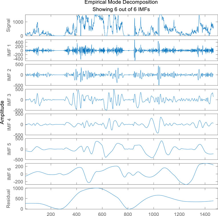
FIGURE 2. EMD decomposition results of the wind power sequence.

Process of the Wind Power Prediction Model

Based on the aforementioned analysis, the steps of wind power prediction model can be summarized as follows:

1) Use EMD to reduce the non-stationarity of wind power series for obtaining different IMF components and a residual component;

2) After the decomposition of original data, an MA-BP neural network-based wind power prediction model is established for each IMF and residual component, respectively, to obtain prediction results of each component;

3) Superimpose the prediction values of each component to acquire the final prediction value of wind power;

4) Compare the predicted values with the actual wind power data, and analyze the effect of each prediction model.

Case Studies

To verify the adaptability and effectiveness of the proposed model, the wind power data from 1 May 2015 to 20 May 2015 are collected from a wind farm in Jiuquan, Gansu Province, China. A total of 1,536 pieces of historical data including wind power, wind speed, and temperature are used in the simulation test, among which, ninety percent of the data are regarded as the train data set and the rest of the data are regarded as the test set. Also, the data are collected at an interval of 10 min. Wind speed and temperature are the input variables of the proposed forecasting model, and wind power is regarded as the output variable of the BP neural network.

Evaluation Index of the Prediction Model Error

In order to effectively evaluate the accuracy of the whole model, root mean squared error (RMSE), mean absolute error (MAE), and mean absolute percentage error (MAPE) are selected as the evaluation index to evaluate the proposed wind power prediction model. Particularly, the specific formulas of RMSE, MAE, and MAPE are as follows:

$E_{\text{RMSE}}=\sqrt{\frac{{{\displaystyle \sum }}_{t=1}^N{(x_{p,t}-x_{m,t})}^2}{N}},(11)$

$E_{\text{MAE}}=\frac{{{\displaystyle \sum }}_{t=1}^N\left|x_{p,t}-x_{m,t}\right|}{N},(12)$

$E_{\text{MAPE}}=\frac{1}{N}{\displaystyle \sum }_{t=1}^N\left|\frac{x_{p,t}-x_{m,t}}{x_{m,t}}\right|,(13)$

where N is the data length of the test data set, $x_{p,t}$ denotes the prediction value of wind-generated power, and $x_{m,t}$ represents the measured power value of the wind farm.

Parameters of the Model Simulation Test on the Prediction Model

In order to illustrate the contribution of EMD, the simulation tests are performed by three models, i.e., standard BP neural network, MA-BP neural network, and combined MA-BP prediction model with EMD. In addition, with the multiple imitation experiments, the specific parameters of each wind power prediction model and EMD algorithm are tabulated in Table 1. In particular, all case studies are implemented by MATLAB 2019b through a personal computer with IntelR CoreTMi5 CPU at 3.0 GHz and 16 GB of RAM.

TABLE 1

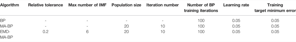
TABLE 1. Parameter settings of each neural network algorithm.

During the simulation experiments, the interpolation method used for envelope construction is Hermite interpolation, and the network structure of designed model is 2, 5, and 1 for each layer (i.e., input, hidden, and output layer).

Result Analysis of the Simulation Test

The wind power curves of three prediction models and actual values are shown in Figure 3, and the corresponding RMSE values of each data point for three prediction models are illustrated in Figure 4. Moreover, the average prediction error (RMSE and MAE) of each prediction model is tabulated in Table 2.

FIGURE 3

FIGURE 3. Predicted power curves of three models.

FIGURE 4

FIGURE 4. RMSE of three wind power prediction models.

TABLE 2

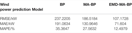
TABLE 2. Average prediction error of each prediction model.

As a whole, with the improvement of the prediction method, the trend of the prediction curve is gradually close to the actual curve, and the prediction accuracy gradually improves. Specifically, the RMSE and MAE decrease from 237.2205 and 191.0634 kW to 107.1728 and 71.604 kW. By analyzing the wind power prediction results based on standard BP and measured power, it is found that the BP network model alone cannot meet the target of forecasting the power output of a wind farm due to its large error from the actual power value. The prediction effect of MA-BP is better than that of BP but still unsatisfactory. In most time periods, the EMD-MA-BP model can fit the actual results well, but it is difficult for the EMD-MA-BP model to make accurate prediction when the wind power changes dramatically due to sudden changes in meteorological conditions. For example, the error of the EMD-MA-BP model is particularly large around the 35th and 110th sampling point in Figure 4.

Conclusion

Wind power prediction is a very complex and challenging work because of the nonlinear and non-stationary characteristics of wind power. As a result, a simple and direct prediction model is difficult to get the ideal prediction effect. To overcome the aforementioned problems, the wind power characteristics should be excavated by hybrid algorithm. Thus, based on the aforementioned ideas, this work proposes a new combined wind power prediction model based on EMD and MA-BP neural network. The following conclusions are obtained from the case studies:

• EMD can effectively reduce the non-stationary characteristics of wind power and is suitable for extracting the characteristics of the wind power curve;

• The abnormal data cleaning based on quartile algorithm is proposed to improve model accuracy;

• The forecasting accuracy of the proposed model based on EMD-MA-BP is higher than that of BP and MA-BP, which reflects the effectiveness of EMD;

• The proposed method is effective in wind power forecasting.

But there is still a lot to improve, and the following work is to develop a noise reduction algorithm for further data preprocessing.

Data Availability Statement

The original contributions presented in the study are included in the article/Supplementary Material; further inquiries can be directed to the corresponding author.

Author Contributions

ZG: conceptualization and writing–reviewing and editing; XM: writing–original draft preparation and investigation; ZC: supervision; YW: conceptualization and resources; CG: writing–reviewing and editing and software; HY: supervision.

Funding

This work was supported in part by the Yunnan Basic Research Project (KKS0202104007) and Key Research Project of China Southern Power Grid (YNKJXM20220011).

Conflict of Interest

Authors ZG, XM, ZC, SZ, YW, CG, and HY were employed in Electric Power Research Institute of Yunnan Power Grid Co., Ltd.

The remaining author declares that the research was conducted in the absence of any commercial or financial relationships that could be construed as a potential conflict of interest.

Publisher’s Note

All claims expressed in this article are solely those of the authors and do not necessarily represent those of their affiliated organizations, or those of the publisher, the editors, and the reviewers. Any product that may be evaluated in this article, or claim that may be made by its manufacturer, is not guaranteed or endorsed by the publisher.

References

Ambach, D., and Schmid, W. (2017). A New High-Dimensional Time Series Approach for Wind Speed, Wind Direction and Air Pressure Forecasting. Energy 135, 833–850. doi:10.1016/j.energy.2017.06.137

CrossRef Full Text | Google Scholar

Chitsaz, H., Amjady, N., and Zareipour, H. (2015). Wind Power Forecast Using Wavelet Neural Network Trained by Improved Clonal Selection Algorithm. Energy Convers. Manag. 89, 588–598. doi:10.1016/j.enconman.2014.10.001

CrossRef Full Text | Google Scholar

Erdem, E., and Shi, J. (2010). ARMA Based Approaches for Forecasting the Tuple of Wind Speed and Direction. Appl. Energy 88 (4), 1405–1414.

Google Scholar

Guchhait, P. K., and Banerjee, A. (2020). Stability Enhancement of Wind Energy Integrated Hybrid System with the Help of Static Synchronous Compensator and Symbiosis Organisms Search Algorithm. Prot. Control Mod. Power Syst. 5 (2), 138–150. doi:10.1186/s41601-020-00158-8

CrossRef Full Text | Google Scholar

Hu, Q., Zhang, R., and Zhou, Y. (2016). Transfer Learning for Short-Term Wind Speed Prediction with Deep Neural Networks. Renew. Energy 85, 83–95. doi:10.1016/j.renene.2015.06.034

CrossRef Full Text | Google Scholar

Huang, N. E., Shen, Z., Long, S. R., Wu, M. C., Shih, H. H., Zheng, Q., et al. (1998). The Empirical Mode Decomposition and the Hilbert Spectrum for Nonlinear and Non-stationary Time Series Analysis. Proc. R. Soc. Lond. A 454 (1971), 903–995. doi:10.1098/rspa.1998.0193

CrossRef Full Text | Google Scholar

Ji, F., Cai, X., and Wang, J. (2014). Wind Power Correlation Analysis Based on Hybrid Copula. Automation Electr. Power Syst. 2, 132–135.

Google Scholar

Jung, J., and Broadwater, R. P. (2014). Current Status and Future Advances for Wind Speed and Power Forecasting. Renew. Sustain. Energy Rev. 31, 762–777. doi:10.1016/j.rser.2013.12.054

CrossRef Full Text | Google Scholar

Kazem, H. A., and Yousif, J. H. (2017). Comparison of Prediction Methods of Photovoltaic Power System Production Using a Measured Dataset. Energy Convers. Manag. 148, 1070–1081. doi:10.1016/j.enconman.2017.06.058

CrossRef Full Text | Google Scholar

Khosravi, H., Samet, H., and Tajdinian, M. (2021). Empirical Mode Decomposition Based Algorithm for Islanding Detection in Micro-grids. Electr. Power Syst. Res. 201, 107542. doi:10.1016/j.epsr.2021.107542

CrossRef Full Text | Google Scholar

Konstantinos, Z., and Stelios, T. (2020). A Mayfly Optimization Algorithm. Comput. Industrial Eng. 145, 106559.

Google Scholar

Li, G., and Shi, J. (2010). On Comparing Three Artificial Neural Networks for Wind Speed Forecasting. Appl. Energy 87 (7), 2313–2320. doi:10.1016/j.apenergy.2009.12.013

CrossRef Full Text | Google Scholar

Liang, Z., Liang, J., Zhang, L., Wang, C., Yun, Z., and Zhang, X. (2015). Analysis of Multi-Scale Chaotic Characteristics of Wind Power Based on Hilbert-Huang Transform and Hurst Analysis. Appl. Energy 159, 51–61. doi:10.1016/j.apenergy.2015.08.111

CrossRef Full Text | Google Scholar

Liu, D., Niu, D., Wang, H., and Fan, L. (2014). Short-term Wind Speed Forecasting Using Wavelet Transform and Support Vector Machines Optimized by Genetic Algorithm. Renew. Energy 62, 592–597. doi:10.1016/j.renene.2013.08.011

CrossRef Full Text | Google Scholar

Liu, H., Tian, H.-q., Chen, C., and Li, Y.-f. (2013). An Experimental Investigation of Two Wavelet-MLP Hybrid Frameworks for Wind Speed Prediction Using GA and PSO Optimization. Int. J. Electr. Power & Energy Syst. 52, 161–173. doi:10.1016/j.ijepes.2013.03.034

CrossRef Full Text | Google Scholar

Liu, Z., Jiang, P., Wang, J., and Zhang, L. (2021). Ensemble Forecasting System for Short-Term Wind Speed Forecasting Based on Optimal Sub-model Selection and Multi-Objective Version of Mayfly Optimization Algorithm. Expert Syst. Appl. 177, 114974. doi:10.1016/j.eswa.2021.114974

CrossRef Full Text | Google Scholar

Ma, S., Jiang, X., and Ma, H. (2013). Algorithm Research on Polishing the Mass Missing Data of Wind Power Based on Regression Model. Adv. Power Syst. Hydroelectr. Eng. 29 (9), 74–80.

Google Scholar

Mahidin, E., Husin, H., Zaki, N. M., et al. (2021). A Critical Review of the Integration of Renewable Energy Sources with Various Technologies. Prot. Control Mod. Power Syst. 6 (1), 37–54.

Google Scholar

Song, D., Yang, J., Fan, X., Liu, Y., Liu, A., Chen, G., et al. (2018). Maximum Power Extraction for Wind Turbines through a Novel Yaw Control Solution Using Predicted Wind Directions. Energy Convers. Manag. 157, 587–599. doi:10.1016/j.enconman.2017.12.019

CrossRef Full Text | Google Scholar

Stevesonn, N., Mesbah, M., and Boashash, B. (2005). “A Sampling Limit for the Empirical Mode Decomposition,”in Proceedings of the Eighth International Symposium on Signal Processing and Its Applications, Sydeny, Australia, 28-31 August 2005 (IEEE), 647–650. doi:10.1109/ISSPA.2005.158102

CrossRef Full Text | Google Scholar

Wang, J., Song, Y., Liu, F., and Hou, R. (2016). Analysis and Application of Forecasting Models in Wind Power Integration: a Review of Multi-Step-Ahead Wind Speed Forecasting Models. Renew. Sustain. Energy Rev. 60, 960–981. doi:10.1016/j.rser.2016.01.114

CrossRef Full Text | Google Scholar

Wang, S., Zhang, N., Wu, L., and Wang, Y. (2016). Wind Speed Forecasting Based on the Hybrid Ensemble Empirical Mode Decomposition and GA-BP Neural Network Method. Renew. Energy 94, 629–636. doi:10.1016/j.renene.2016.03.103

CrossRef Full Text | Google Scholar

Wu, J., Wang, J., Lu, H., Dong, Y., and Lu, X. (2013). Short Term Load Forecasting Technique Based on the Seasonal Exponential Adjustment Method and the Regression Model. Energy Convers. Manag. 70, 1–9. doi:10.1016/j.enconman.2013.02.010

CrossRef Full Text | Google Scholar

Yang, B., Ye, H., Wang, J., Li, J., Wu, S., Li, Y., et al. (2021). PV Arrays Reconfiguration for Partial Shading Mitigation: Recent Advances, Challenges and Perspectives. Energy Convers. Manag. 247, 114738. doi:10.1016/j.enconman.2021.114738

CrossRef Full Text | Google Scholar

Yang, B., Zhong, L., Wang, J., Shu, H., Zhang, X., Yu, T., et al. (2021). State-of-the-art One-Stop Handbook on Wind Forecasting Technologies: an Overview of Classifications, Methodologies, and Analysis. J. Clean. Prod. 283, 124628. doi:10.1016/j.jclepro.2020.124628

CrossRef Full Text | Google Scholar