Small-Signal Distributed Frequency Modeling and Analysis for Grid-Forming Inverter-Based Power Systems

More and more renewable energy sources are integrated into power grids, leading to a power electronic-based low-inertia power system. The grid-forming (GFM) inverter is an effective method for improving the inertia of the system. However, with the increased GFM inverters in the system, how the multiple control parameters affect the frequency response is still not clear. In this study, first, the power-phase model of the power grid is established; then, a small-signal distributed frequency model of the GFM inverter-based power system is established associating with the power-phase model of the power grid and the power-frequency model of the GFM inverter. Based on the proposed model, the influence of the multiple parameters to the frequency response is analyzed. It is concluded that both the inertia and damping coefficient affect the settling time, overshoot, and oscillation of the frequency. Finally, the simulation results verify the proposed model and the conclusion.

Introduction

Recently, more and more renewable energy sources (RESs) have been developed to alleviate the increasingly tight power supply of fossil energy (Huang et al., 2011). These RESs adopt the inverter as the interface connected to the power grid. The inverter grid-connected control can be classified into two types: the grid-following (GFL) and grid-forming (GFM) controls. The GFL inverter lacks the inertia and damping compared to the traditional synchronous generator (Liu et al., 2016). Therefore, the increased penetration of RESs has greatly decreased the overall inertia level of the power system, which raises great challenges to the stability of the system, especially for the low-inertia system, such as the microgrid in the islanded mode (Alipoor et al., 2018). To address this problem, the GFM control is considered to be a simple and effective approach for improving the inertia of the system (Quan et al., 2020a) (Quan, 2021) (Wu et al., 2016). The well-known virtual synchronous generator (VSG) control belongs to the GFM control methods (Wu et al., 2016).

The GFM inverter usually adopts power synchronization control which includes the two parameters of inertia and damping (Quan et al., 2020b). These two parameters play critical roles in improving the performance and maintaining the stability of the power system. Compared with the synchronous generator, the virtual inertia and damping coefficient of the GFM inverter are realized in the control software; hence, they are flexible and adjustable. The design of the inertia and damping for a single GFM inverter has been studied well (Wu et al., 2016), (Quan et al., 2020b). However, how to optimally determine the virtual inertia and damping coefficient for multiple GFMs in a GFM-based power system to get better stability and dynamic performance is still a challenge.

To optimally design the multiple inertias and damping factors, a suitable model should be established first. However, for such a large nonlinear system, the small-signal model is suitable for the optimal design of virtual inertia and damping coefficient. A grid-forming inverter-based power system is comprehensively modeled in (Pogaku et al., 2007), where the small-signal stability issues are analyzed by plotting zero-pole locations. Based on the grid-forming technology, many stability performances in terms of regulating frequency and voltage can be achieved, for example, asymptotical (Bidram et al., 2013) and finite-time (Ge et al., 2021). However, these studies consider the control design from the perspective of a power electronic-based inverter and do not fully consider the interaction between grid-forming inverters and power networks.

Based on the traditional small-signal modeling method, a detailed system model including grid-following inverters and grid-forming inverters is built with the node admittance matrix, and a H₂ norm-based control algorithm is proposed to optimize the virtual inertia in order to improve the stability of the low-inertia power system (Poolla et al., 2019). However, the nodal admittance matrix cannot describe how the load power fluctuation affects the system frequency in an explicit way. Hence, it is not conducive to the parameter optimization. Differently, a model with multiple GFMs was established by using direct current power flow in Ademola-Idowu and Zhang, 2018, and the optimized design of the virtual inertia and damping coefficient was also described as a H₂ norm minimization problem. A more detailed demonstration was proposed in Mešanović et al., 2016 for the system model using DC power flow, based on which a comparison among the H_∞, H₂, and pole optimizations for damping active power oscillations was presented. Nevertheless, the DC power flow algorithm is not applicable for a low-voltage microgrid or low-inertia system where most DGs are connected (Frack et al., 2015) (Kundur, 1994).

Therefore, this study proposes a state space small-signal model for the multi-GFM system. Based on the proposed model, the relationship between the load fluctuation and frequency change is explicitly expressed, which is beneficial to the numerical optimization of the parameters of virtual inertia and damping coefficient. Moreover, the dynamic characteristic of the frequency is also demonstrated by the proposed state space model. Finally, the influence of the parameters on the dynamic response is analyzed and verified.

Modeling for the Grid-Forming-Based System

System Description

As shown in Figure 1, in an inverter-based power system, the GFM inverter is necessary to form the AC voltage. Under these conditions, the swing-equation-based power control or power synchronization control will be applied to realize the frequency synchronization and power sharing. Consequently, the control parameters of the power control, for example, the damping factor and virtual inertia, will remarkably affect the system frequency dynamics. Moreover, due to the difference of these power control parameters, the frequency of the system will demonstrate the features of distribution. Hence, it is meaningful to establish a dynamic model to describe the frequency dynamics of the system.

FIGURE 1

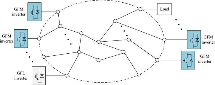
FIGURE 1. Diagram of the GFM inverter-based power system.

As shown in Figure 2, the system nodes are divided into two types. One is the node that is connected with GFM inverters, and it is called the GFM-node. The voltage and frequency of the GFM-node are determined by the GFM inverter. The last nodes are classified into one type that injects active and reactive power into the node. In this study, these nodes are treated as the disturbance nodes.

FIGURE 2

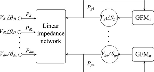
FIGURE 2. Diagram of the inverter-based power system.

Modeling of the Grid-Forming Inverter

The GFM active power control part simulates the inertia, droop characteristics, and damping action of the synchronous machine. It is assumed that the GFM active power control equation similar to the second-order rotor motion equation of the synchronous machine can be expressed as Eq. 1

$\{\begin{array}{l}\frac{d\mathrm{\Delta }{\theta }_{gi}}{dt}=\mathrm{\Delta }{\omega }_{gi}\\ M_i\frac{\mathrm{d}\mathrm{\Delta }{\omega }_i}{\mathrm{d}\mathrm{t}}=\frac{P_{\mathrm{s}\mathrm{e}\mathrm{t},i}-P_{gi}}{{\omega }_{\mathrm{n}}}-D_{p,i}\mathrm{\Delta }{\omega }_{gi}\\ {\omega }_{gi}=\mathrm{\Delta }{\omega }_{gi}+{\omega }_{\mathrm{n}}\end{array}(1)$

where Δθ_gi denotes the phase variation of GFM node i at the current operation point, M_i is the virtual inertia of the i-th GFM inverter, D_p,i is the damping coefficient, P_set,i is the set value of active power, P_gi is the output active power, ω_n is the rated angular frequency, and ω_gi is the angular frequency of the i-th GFM inverter. Considering all the GFM nodes, Eq. 1 can be written in matrix formation:

$\{\begin{array}{c}\frac{d\mathrm{\Delta }{\mathit{\theta }}_g}{dt}=\mathrm{\Delta }{\omega }_g\\ \frac{d\mathrm{\Delta }{\omega }_g}{dt}=\frac{{\mathit{M}}^{-1}}{{\omega }_n}\left({\mathit{P}}_{set}-{\mathit{P}}_g\right)-{\mathit{M}}^{-1}{\mathit{D}}_p\mathrm{\Delta }{\mathit{\omega }}_g\end{array}(2)$

Modeling of the Power Grid

To establish the model of the GFM inverter-based system, how the phase angles of the GFM inverters and the injected power of disturbance nodes affect the power of the GFM inverter through the impedance network needs to be clarified. To this end, the Jacobian matrix is adopted:

$\left[\begin{array}{c}\mathrm{\Delta }\mathit{P}\\ \mathrm{\Delta }\mathit{Q}\end{array}\right]=\left[\begin{array}{cc}\mathit{H}& \mathit{N}\\ \mathit{J}& \mathit{L}\end{array}\right]\left[\begin{array}{c}\mathrm{\Delta }\mathit{\theta }\\ \mathrm{\Delta }\mathit{V}/\mathit{V}\end{array}\right](3)$

where matrices H, N, J, and L are derived from the fundamental power flow equations. In the high-voltage power system, it has N = 0 and J = 0, which means that the voltage is related with the reactive power, while the frequency is dependent on the active power. Hence, the influence of the reactive power can be ignored when analyzing the frequency dynamics. Then, Eq. 3 is simplified as

$\left[\begin{array}{c}\mathrm{\Delta }{P}_1\\ \mathrm{\Delta }{P}_2\\ ⋮\end{array}\right]=\left[\begin{array}{ccc}{H}_{11}& H_{12}& \cdots \\ H_{21}& H_{22}& \cdots \\ ⋮& ⋮& \ddots \end{array}\right]\left[\begin{array}{c}\mathrm{\Delta }{\theta }_1\\ \mathrm{\Delta }{\theta }_2\\ ⋮\end{array}\right](4)$

where ΔP_i and Δθ_i denote the power and phase variation of node i at the current operation point, respectively. The elements of the matrix are linearized from the fundamental power equation:

$\{\begin{array}{c}{H}_{ij}=\frac{\partial P_i}{\partial {\delta }_j}=U_i{U}_j\left(G_{ij}\sin {\delta }_{ij}-B_{ij}\cos {\delta }_{ij}\right)\begin{array}{cc},& i\ne j\end{array}\\ H_{ii}=\frac{\partial P_i}{\partial {\delta }_i}=-U_i{\displaystyle \sum _{j=1,j\ne i}^{j=n}{U}_j\left(G_{ij}\sin {\delta }_{ij}-B_{ij}\cos {\delta }_{ij}\right)\begin{array}{cc},& i=j\end{array}}\end{array}(5)$

Distinguishing the GFM nodes and disturbance nodes, Eq. 4 can be rearranged as

$\left[\begin{array}{c}\mathrm{\Delta }{\mathit{P}}_{\mathit{g}}\\ \mathrm{\Delta }{\mathit{P}}_d\end{array}\right]=\left[\begin{array}{cc}{\mathit{H}}_{gg}& {\mathit{H}}_{gd}\\ {\mathit{H}}_{dg}& {\mathit{H}}_{dd}\end{array}\right]\left[\begin{array}{c}\mathrm{\Delta }{\mathit{\theta }}_g\\ \mathrm{\Delta }{\mathit{\theta }}_d\end{array}\right](6)$

Integrated Model

The phase angle vector of the GFM nodes Δθ_g is the state variable of the system, while Δθ_d is the dependent variable. The power of the disturbance node will be the disturbance that occurs with the phase angle and frequency variations. To extract the disturbance from Eq. 6, Kron reduction is applied to Eq. 6, obtaining

$\mathrm{\Delta }{\mathit{P}}_g=\left({\mathit{H}}_{gg}-{\mathit{H}}_{gd}\mathit{H}\frac{-1}{dd}{\mathit{H}}_{dg}\right)\mathrm{\Delta }{\mathit{\theta }}_g+{\mathit{H}}_{gd}\mathit{H}\frac{-1}{dd}\mathrm{\Delta }{\mathit{P}}_d(7)$

Then, combining Eqs. 2 and 7, it has

$\frac{d}{dt}\left[\begin{array}{c}\mathrm{\Delta }{\mathit{\theta }}_g\\ \mathrm{\Delta }{\mathit{\omega }}_g\end{array}\right]=\left[-{\left({\omega }_n\mathit{M}\right)}^{-1}\left({\mathit{H}}_{gg}-{\mathit{H}}_{gd}{\mathit{H}}_{dd}^{-1}{\mathit{H}}_{dg}\right)\begin{array}{c}\mathit{I}\\ -{\mathit{M}}^{-1}{\mathit{D}}_p\end{array}\right]\left[\begin{array}{c}\mathrm{\Delta }{\mathit{\theta }}_g\\ \mathrm{\Delta }{\mathit{\omega }}_g\end{array}\right]+\left[\begin{array}{c}0\\ -{\left({\omega }_n\mathit{M}\right)}^{-1}{\mathit{H}}_{gd}{\mathit{H}}_{dd}^{-1}\end{array}\right]\mathrm{\Delta }{\mathit{P}}_d+\left[\begin{array}{c}0\\ -{\left({\omega }_n\mathit{M}\right)}^{-1}\end{array}\right]{\mathit{P}}_{set}(8)$

which is the space state model of the system. The state variables Δθ_g and Δω_g represent the dynamics of the phase angle and frequency of the GFM nodes. Therefore, we can conveniently evaluate the dynamic response of the frequency for every GFM node during the dynamic process. Thereby, we can optimally design the control parameters of the GFM power controller.

Pole Analysis

In this section, the proposed model is applied to a 9-buses system as shown in Figure 3. Three GFM inverters are connected at bus 1, bus 2, and bus 3. Three loads are connected at bus 5, bus 7, and bus 9. The parameters are listed in Table 1.

FIGURE 3

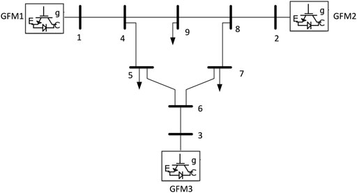
FIGURE 3. Diagram of in the 9-buses system.

TABLE 1

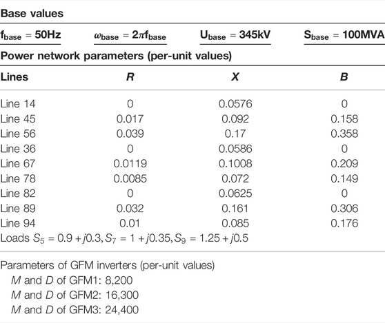
TABLE 1. | Parameters of the system and the inverters.

Using the concrete parameters of the 9-buses system shown in Figure 3, the model of Eq. 8 can be obtained. Then, based on the model, the root locus when the inertias vary is investigated. The inertia and damping parameters for the three GFM inverters are denoted as M = (M₁, M₂, M₃) and D_p = (D_p,1, D_p,2, D_p,3) for GFM1, GFM2, and GFM3. Figure 4A–C shows the pole variation when the inertia parameter of the three GFM inverters changes. Generally, the poles of the system rule the dynamic response of the frequency. Each pair of the conjugate poles has the parameters of damping factor and damping oscillation frequency (the real part of the pole). The high damping factor can reduce the oscillation and overshoot during the dynamic response. The large damping oscillation frequency reduces the settling time, which means that it increases the response speed. As can be seen in Figure 4A–C, with the inertia increasing, all of the poles move toward the imaginary axis, which means that the response will become slow. It is reasonable since the inertia is increased. Moreover, the damping factor is reduced due to the increased inertia. This will enhance the overshoot and oscillation.

FIGURE 4

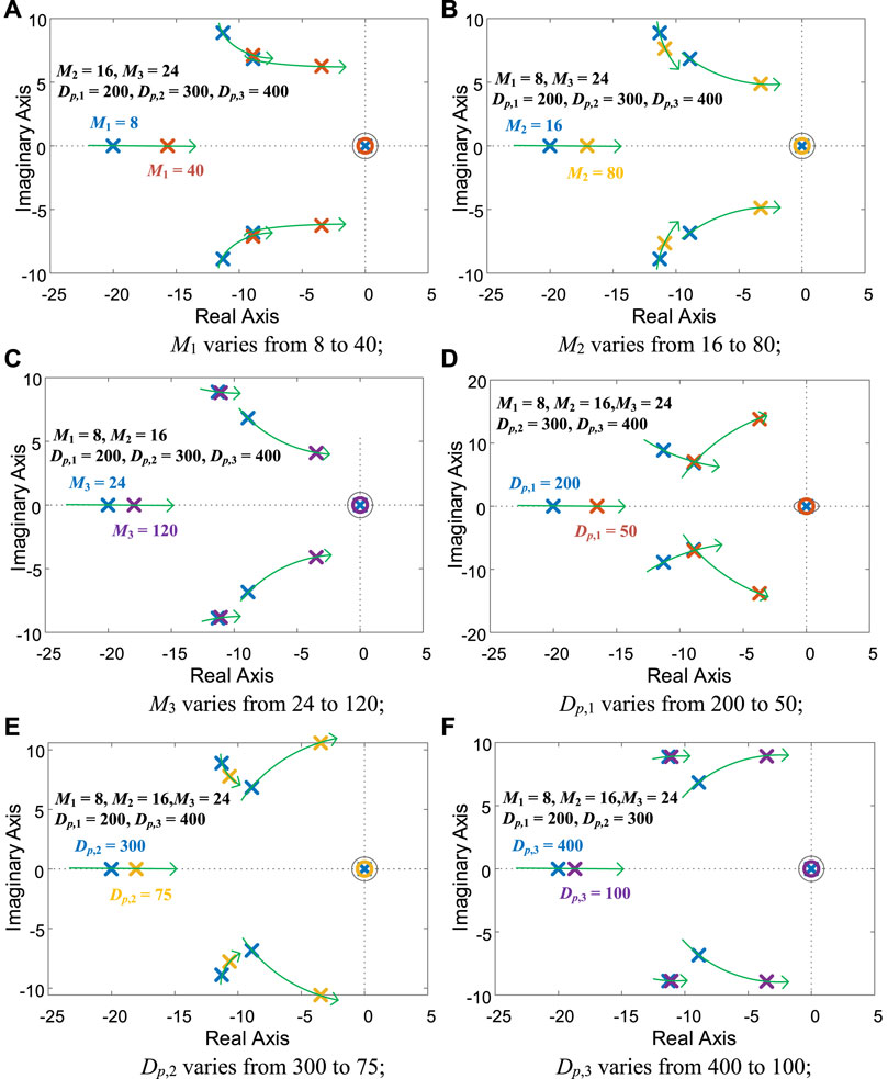
FIGURE 4. Root locus of the system when the parameters vary.

Figure 4D–F shows how the damping factor affects the poles. Generally, the damping factors reflect the droop coefficient; hence, they are usually designed by the frequency support capacity. However, from Figure 4D–F, it is shown that the damping factors also influence the dynamic response. With the damping factor decreasing (frequency supporting capacity decreasing), the poles move toward the imaginary axis, which means that the response will become slow; meanwhile, the damping becomes worse. It will cause severe overshoot and oscillation on frequency dynamics.

Simulation Results

Model Verification

To verify the correctness of the proposed model, the electrical simulation in Simulink is conducted as a comparison. The adopted parameters are M = (8, 16, 24) and D_p = (200, 300, 400). The disturbance appeared on node 7 with 0.01 p.u. active power increase. As shown in Figure 5, the frequency responses of the electrical simulation and the proposed small-signal model demonstrate that the dynamic feature of the frequency can be perfectly described by the proposed small-signal model. However, there is a small steady-state error which appears on the proposed small-signal model. This is introduced by the linearization of the Jacobian matrix. Nevertheless, the steady-state value can be obtained by the direct static-state droop computation. Hence, the dynamic feature described by the proposed model can still be adopted optimally to design the control parameters of the GFM inverters.

FIGURE 5

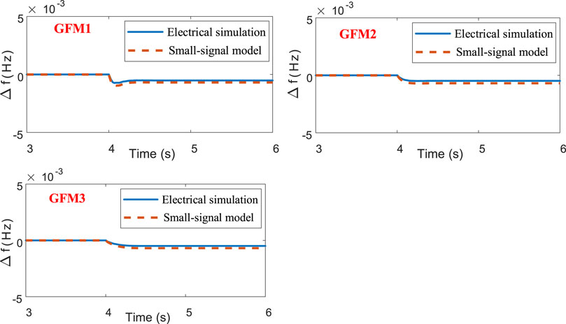
FIGURE 5. Frequency response of the electrical simulation and the proposed small-signal model.

Performance Verification

Furthermore, to evaluate the effect of the control parameters to the frequency performance, the simulation with different parameters is performed. Figure 6 shows the different frequency dynamic responses with the inertia variations, and the pole figures are also displayed for a reference. In Figure 6, the first column shows that the inertia of GFM1 changes from 8 to 40, while the other parameters stay invariable. The second column shows that the inertia of GFM2 changes from 16 to 80, and the third column shows the inertia of GFM3 changes from 24 to 120. From the results in Figure 6, first, it is concluded that the inertia only affects its own rate of change of frequency (RoCoF) but has no effect on the RoCoF of the other node; increasing the inertia of GFM1 only reduces the RoCoF of GFM1 but without the influence of RoCoFs of GFM2 and GFM3. Second, increasing the inertia will move the poles right, which increases the settling time; all the settling times of the frequencies for the three inverters become larger. Third, increasing the inertia also decreases the damping of the system; hence, the oscillation and overshoot of the frequencies of the three inverters are deteriorated.

FIGURE 6

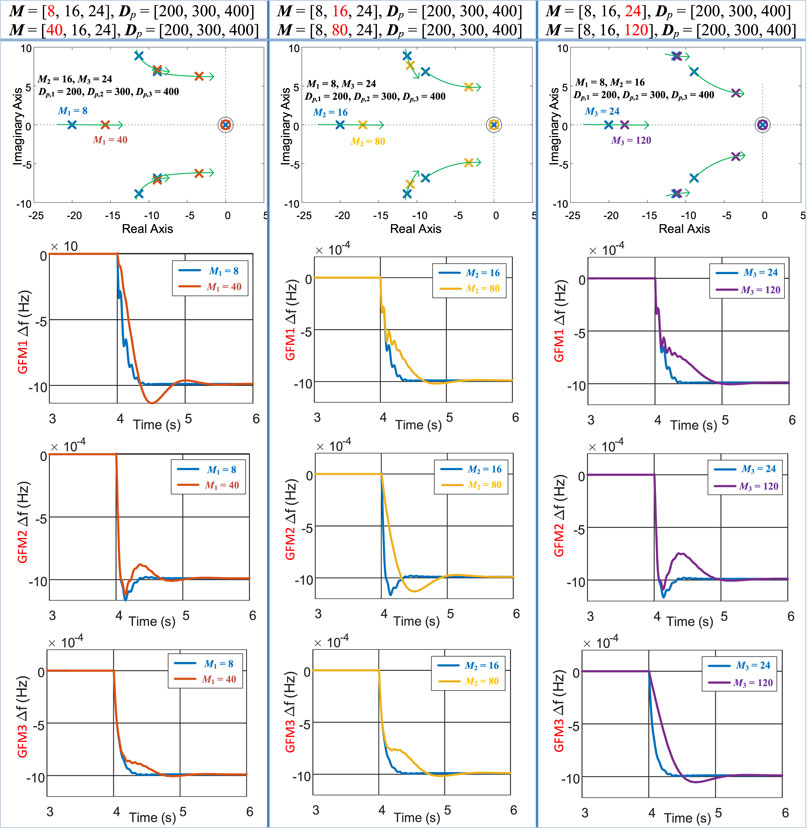
FIGURE 6. Frequency response when the inertia changes.

Figure 7 shows the distributed frequency response of different GFM inverters when the damping coefficients change. The first column shows that the damping coefficient of GFM1 changes from 200 to 50, while the other parameters stay invariable. The second column shows that the damping coefficient of GFM2 changes from 300 to 75, and the third column shows that the damping coefficient of GFM3 changes from 400 to 100. Observing the frequency waveforms in Figure 7, first, we can conclude that the damping coefficient still acts as the droop coefficient that denotes the frequency supporting capacity. Hence, reducing the damping coefficients will reduce the frequency steady-state value. Second, the reduced damping coefficient moves the pole toward the imaginary axis; hence, the settling time becomes larger with the reduced damping coefficient. Third, decreasing the damping coefficient decreases the damping of the system; hence, the oscillation and overshoot of the frequencies of the three inverters are deteriorated. Last, the damping coefficient has no effect on the RoCoFs of the frequency.

FIGURE 7

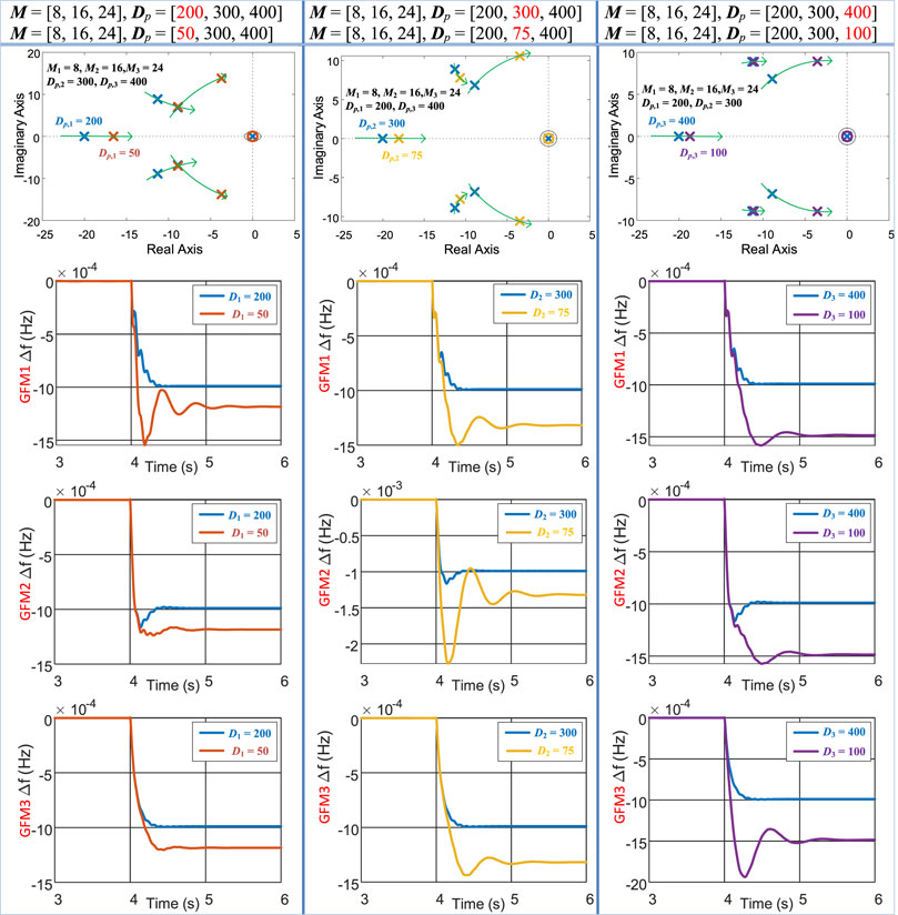
FIGURE 7. Frequency response when the damping changes.

Moreover, to comprehensively evaluate the effectiveness of the proposed model, the load power disturbance is imposed on different nodes. Figure 8 shows the frequency response when the load steps 0.01 p.u. active power. The parameters of the inverters are set as M = (8 16 24) and D = (200 300 400). As shown in Figure 8, the frequency of GFM2 and GFM3 performs a good dynamic response, while the frequency of GFM1 shows a large overshoot. This because that the inertia of GFM1 is set too small, which occurs as a poor damping factor of the corresponding poles.

FIGURE 8

FIGURE 8. Frequency response with different load variations.

Conclusion

In this study, a state space small signal model is established for the multiple GFM low-inertia system. The system is modeled in an input–output state space model where the load power is the disturbance input and the frequency of every node is the output. The proposed model can perfectly describe the dynamic feature of the frequency. From the proposed model, it is concluded that increasing the inertia and reducing the damping coefficient will increase the settling times of the frequencies, deteriorate the oscillation, and overshoot of the frequencies. Moreover, increasing the inertia will decrease the RoCoF of its own node frequency, while the damping coefficient has no effect on the RoCoFs of the frequency.

Furthermore, the proposed model is based on the small-signal stability theory; therefore, it is limited to analyze the large-signal stability. In the future work, we will focus on the suitable model for a large-signal stability analysis.

Data Availability Statement

The original contributions presented in the study are included in the article/supplementary material; further inquiries can be directed to the corresponding author.

Author Contributions

XQ: Model establishment, running the simulation, and writing the paper. JZ: Advising and revising the paper. FM: Advising and revising the paper.

Funding

This study was funded by the Key R&D plan of Jiangsu Province (BE2020027) and in part by the Jiangsu International Science and technology cooperation project (BZ2021012).

Conflict of Interest

The authors declare that the research was conducted in the absence of any commercial or financial relationships that could be construed as a potential conflict of interest.

The reviewer YJ declared a shared affiliation with the authors XQ and JZ to the handling editor at the time of review.

Publisher’s Note

All claims expressed in this article are solely those of the authors and do not necessarily represent those of their affiliated organizations or those of the publisher, the editors, and the reviewers. Any product that may be evaluated in this article or claim that may be made by its manufacturer is not guaranteed or endorsed by the publisher.

References

Ademola-Idowu, A., and Zhang, B. (2018). “Optimal Design of Virtual Inertia and Damping Coefficients for Virtual Synchronous Machines,” in 2018 IEEE Power & Energy Society General Meeting (PESGM), Portland, OR, USA, 5-10 Aug. 2018 (IEEE), 1–5. doi:10.1109/PESGM.2018.8586187

CrossRef Full Text | Google Scholar

Alipoor, J., Miura, Y., and Ise, T. (2018). Stability Assessment and Optimization Methods for Microgrid with Multiple VSG Units. IEEE Trans. Smart Grid 9 (2), 1462–1471. doi:10.1109/tsg.2016.2592508

CrossRef Full Text | Google Scholar

Bidram, A., Davoudi, A., Lewis, F. L., and Guerrero, J. M. (2013). Distributed Cooperative Secondary Control of Microgrids Using Feedback Linearization. IEEE Trans. Power Syst. 28, 3462–3470. doi:10.1109/tpwrs.2013.2247071

CrossRef Full Text | Google Scholar

Frack, P. F., Mercado, P. E., Molina, M. G., Watanabe, E. H., De Doncker, R. W., and Stagge, H. (2015). Control Strategy for Frequency Control in Autonomous Microgrids. IEEE J. Emerg. Sel. Top. Power Electron. 3 (4), 1046–1055. doi:10.1109/jestpe.2015.2439053

CrossRef Full Text | Google Scholar

Ge, P., Zhu, Y., Green, T. C., and Teng, F. (2021). Resilient Secondary Voltage Control of Islanded Microgrids: An ESKBF-Based Distributed Fast Terminal Sliding Mode Control Approach. IEEE Trans. Power Syst. 36 (2), 1059–1070. doi:10.1109/TPWRS.2020.3012026

CrossRef Full Text | Google Scholar

Huang, A. Q., Crow, M. L., Heydt, G. T., Zheng, J. P., and Dale, S. J. (2011). The Future Renewable Electric Energy Delivery and Management (FREEDM) System: The Energy Internet. Proc. IEEE 99 (1), 133–148. doi:10.1109/jproc.2010.2081330

CrossRef Full Text | Google Scholar

Kundur, P. (1994). Power System Stability and Control. New York: McGraw-Hill.

Google Scholar

Liu, J., Miura, Y., and Ise, T. (2016). Comparison of Dynamic Characteristics between Virtual Synchronous Generator and Droop Control in Inverter-Based Distributed Generators. IEEE Trans. Power Electron. 31 (5), 3600–3611. doi:10.1109/tpel.2015.2465852

CrossRef Full Text | Google Scholar

Mešanović, A., Münz, U., and Heyde, C. (2016). Comparison of H_∞, H₂, and Pole Optimization for Power System Oscillation Damping with Remote Renewable Generation. IFAC Workshop Control Transm. Distribution Smart Grids CTDSG 49 (27), 103–108. doi:10.1016/j.ifacol.2016.10.727

CrossRef Full Text | Google Scholar

Pogaku, N., Prodanovic, M., and Green, T. C. (2007). Modeling, Analysis and Testing of Autonomous Operation of an Inverter-Based Microgrid. IEEE Trans. Power Electron. 22 (2), 613–625. doi:10.1109/TPEL.2006.890003

CrossRef Full Text | Google Scholar

Poolla, B. K., Dorfler, D., and Dörfler, F. (2019). Placement and Implementation of Grid-Forming and Grid-Following Virtual Inertia and Fast Frequency Response. IEEE Trans. Power Syst. 34 (4), 3035–3046. doi:10.1109/tpwrs.2019.2892290

CrossRef Full Text | Google Scholar

Quan, X., Huang, A. Q., and Yu, H. (2020). A Novel Order Reduced Synchronous Power Control for Grid-Forming Inverters. IEEE Trans. Ind. Electron. 67 (12), 10989–10995. doi:10.1109/tie.2019.2959485

CrossRef Full Text | Google Scholar

Quan, X. (2021). Improved Dynamic Response Design for Proportional Resonant Control Applied to Three-phase Grid-Forming Inverter. IEEE Trans. Ind. Electron. 68 (10), 9919–9930. doi:10.1109/TIE.2020.3021654

CrossRef Full Text | Google Scholar

Quan, X., Yu, R., Zhao, X., Lei, Y., Chen, T., Li, C., et al. (2020). Photovoltaic Synchronous Generator: Architecture and Control Strategy for a Grid-Forming PV Energy System. IEEE J. Emerg. Sel. Top. Power Electron. 8 (2), 936–948. doi:10.1109/JESTPE.2019.2953178

CrossRef Full Text | Google Scholar

Wu, H., Ruan, X., Yang, D., Chen, X., Zhao, W., Lv, Z., et al. (2016). Small-signal Modeling and Parameters Design for Virtual Synchronous Generators. IEEE Trans. Ind. Electron. 63 (7), 4292–4303. doi:10.1109/tie.2016.2543181

CrossRef Full Text | Google Scholar