The classification model for identifying single-phase earth ground faults in the distribution network jointly driven by physical model and machine learning

Single-phase earth ground faults are the most frequent faults likely to occur but hard to identify in a distribution system, especially in a neutral ineffectively grounded system. Targeting on this goal, a novel AdaBoost-based single-phase earth ground fault identification model is put forward. First, after depicting the zero-sequence circuit of the distribution system, a feature engineering that can reflect local and global evolutionary processes in the fault period is constructed in detail. Second, to overcome two problems, namely, different number problems between fault and non-fault samples and curse of dimension, principal component analysis is used for feature extraction, in which only a small number of low-dimension mapped features are extracted, and then transmitted into the AdaBoost-based ground fault identification model. Subsequently, this work borrows from machine learning and applies its learning curve and receiver operating characteristic curve to guide the optimization of the proposed identification model. Numerical studies verify the effectiveness and adaptability of the proposed model toward solving single-phase earth ground faults.

1 Introduction

In extreme short-circuit situations, designing feeder relays would be simple in general. However, the single-phase earth ground fault is out of this category, especially in low- and medium-voltage distribution networks (3∼66 kV) with ineffectively grounded neutral points (Cui et al., 2011; Xue et al., 2015). In this regard, it is also referred to as a small-current grounded system. In contrast with other short-circuit faults, single-phase earth ground faults are mostly to happen, and by incomplete statistics, they account for around 60%∼80%. Interestingly, most interphase faults are the deteriorated outcomes of single-phase earth ground faults. Therefore, detecting this “weak” earth fault is very important for protection engineers in order to prevent more severe hazards and to ensure the safety and reliability of power delivery.

Most scholars have conducted many studies in this field. So far, some staged and conclusive achievements have been made. Specifically, the approach in identification single-phase earth ground fault can be normally categorized into two mainstream branches: steady-state method and transient method. As for the former, it includes six sub-approaches (Xu et al., 2005; Ai et al, 2009; Gautam and Brahma, 2012; Li, 2017): zero-sequence current amplitude comparison method, zero-sequence current phase comparison method, fifth harmonic component method, zero-sequence active power component method, zero-sequence reactive power method, and zero-sequence admittance method. The main principal of these methods is that zero-sequence current of the fault line is the summation of all non-fault lines, and it shall be larger than any of other lines. Considering the line-to-ground conductance and the resistance loss of an arc suppression coil, a new protection criterion is established via recognizing the direction difference of active power (Xu et al., 2005; Li, 2017). Although not limited to the arc suppression coil, its active component is generally small, especially when the three-phase imbalance degree is relatively large, it will be easier to misjudge faults due to the false active current component. With respect to the transient method, it includes three parts: first half-wave polarity method, transient power direction method, and transient parameter identification method (Yao and Cao, 2009; Zeng et al., 2012). Compared with the former, this method is relatively less influenced by the form that the neutral point is grounded or noneffective. From this perspective, it possesses better adaptability (Zhu, 2011). Hence, it has been gradually becoming more important and popular in this single-phase earth ground fault identification field, especially as the function of transient-recording-type devices is becoming a mainstream product (Jiale et al., 2007; Zhang and Yin, 2011; Ghaderi et al., 2017).

Moreover, revolving around this target, there are several novel techniques, such as three-phase current method and transient frequency band method. Specifically, Song et al. (2011) propose the three-phase current method, which collects the sudden change of three-phase current in a transient process, calculates the relevant coefficients between each pair of phases, and subsequently discriminates the ground fault according to the fault phase that has the smallest relevance degree. As for the latter, some scholars have proposed a method of extracting information of specific frequency in transient zero-sequence current and then identifying single-phase earth ground faults by comparing the difference between the amplitude and polarity (Xue et al., 2003; Liu et al., 2018). An et al. (2020) propose the grounding protection principle based on half-wave Fourier algorithm and establish an action criterion algorithm model based on half-wave Fourier algorithm. Shu et al. (2019) propose the wavelet transform method to realize the extraction of transient zero-sequence information. Lishan et al. (2020) propose a fault line identification scheme with admittance asymmetry parameters as the criterion and utilize the fifth harmonic principle to solve the issue regarding the disappearance of fault differences between the fault lines and non-fault lines of the neutral point after passing through the extinction coil grounding system. He et al. (2017) identify grounding faults by using relative entropy of the generalized S-transform energy of zero-sequence current. Zhou (2016) establishes a dynamic grounding fault sensing criterion based on the features of injection current variables after fault occurrence and identifies fault lines by comparing the effective value of zero-sequence current variables of different feeders. Although these transient signal methods produce ideal effects in handling faults with a large zero-sequence current, they are likely to be affected by systematic influences in multiple processes (e.g., constant startup value, sampling noise, and electromagnetic interference, etc.) during actual operation when fault zero-sequence current is low, leading to low algorithmic sensitivity. They are too easily affected by operating conditions of the distribution network and rely excessively on the differential configuration of various configuration parameters.

In fact, the issue of identifying faults can be viewed as the scope of classification, for which it is highly relevant to machine learning (e.g., clustering, classification, and regression under the semi-supervised/supervised mode). Recently, machine learning technology has developed rapidly. With reference to the 2016 International Summit on Application of Machine Learning Industry jointly held by IBM and CDA Data Analysis and Research Institute, this has been applied in many fields, for e.g., finance, IT, computers, and transportation, and has proven to be extraordinarily valuable. In view of this, some researchers are working on building an intelligent fault identification model via machine learning technology (Wang et al., 2021). Although relatively reliable identification results have been elementarily achieved, the lack of hyperparameter adjustment, over/underfitting judgment, and feature extraction in optimizing the identification model is its critical defect. In general, exploring the application of machine learning in the fault identification field requires more systematic and theoretical discussions in depth.

In light of the aforementioned background, this article borrows from machine learning and puts forward a novel single-phase earth ground fault identification method jointly driven by practical fault data and Simulink model.

Major contributions of this article include:

1) In reflecting the local and global evolutional process of fault features and forms, this article chooses two major fault features (including their amplitudes, delta variations and phase degrees), which could form an entire feature engineering taking the stable/transient state of the faulty network into account.

2) In combination with machine learning, a mainstream feature reduction method of principal component analysis (PCA) is applied into which feature reduction of high-dimension fault features can in validity select only a small number of but key mapped features of potential values and further elevate model identification efficiency in engineering practice.

3) AdaBoost-based single-phase earth fault identification model is designed in this work into which the features of high priority are fed, where several manners of learning curve, validation curve, and receiver operating characteristic curve (ROC) are all brought out into guiding model optimization, and thus an entire fault identification technology based on machine learning is gradually formed. Additionally, model performance is quantitively analyzed from the perspective of accuracy and area under the curve (AUC) indicators.

The remainder of this article is organized as follows: in Section 2 depicts the equivalent circuit diagram of a distribution system when a single-phase earth ground fault occurs in this system and constructs the ground fault feature engineering. Next, a machine-learning-based ground fault identification model is built. To overcome its underfitting/overfitting possibilities, some hyperparameter optimization techniques have been applied, such as up-sampling technology, feature reduction, learning/validation curve, and receiver operating characteristic curve (ROC). Finally, the practical dataset and the Simulink dataset are both used as learning samples in the Numerical studies part, and in this section, it demonstrates the validity and adaptability of the proposed ground fault identification model under multiple scenarios.

2 Feature engineering of single-phase earth ground faults

2.1 Physical model of single-phase grounding faults

To construct reasonable and complete fault features, this section will analyze the change features of system parameters in single-phase earth ground faults, like the capacitance current distribution in the system, from the perspective of the circuit of the distribution network. The distribution of capacitance current during single-phase grounding is shown in Figure 1. In Figure 1: $C_{OG}$, $C_{OI}$, and ${\mathrm{C}}_{\mathrm{O}\mathrm{I}\mathrm{I}}$ are the capacitive parameters over the ground of each generator, line I, and line II, respectively; ${\dot{I}}_{BG}$ and ${\dot{I}}_{CG}$ are, respectively, the capacitive parameters over the ground of phase B and phase C on generator G; ${\dot{I}}_{BI}$ and ${\dot{\mathrm{I}}}_{\mathrm{C}\mathrm{I}}$ are, respectively, the capacitive parameters over the ground of phase B and phase C on line I; and ${\dot{I}}_{BII}$ and ${\dot{\mathrm{I}}}_{\mathrm{C}\mathrm{I}\mathrm{I}}$ are, respectively, the capacitive parameters over the ground of phase B and phase C on line I.

FIGURE 1

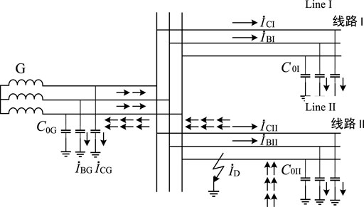
FIGURE 1. Capacitance current distribution represented by the three-phase system during single-phase grounding.

In combination with information from Figure 1, it can be seen that the voltage drop of load current and capacitance current on line impedance can be ignored after phase A of line II is grounded. It can be inferred that capacitance current over the ground of phase A of all element equipment also equals zero when phase A of the entire system is grounded, and voltage and capacitance current over the ground of phase B and phase C are increased by 1.732 times. The distribution of the capacitance current under such circumstances is as shown in “→” of Figure 1. The zero-sequence equivalent network and phasor network of single-phase grounding are, respectively, depicted in Figures 2A,B.

FIGURE 2

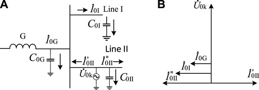
FIGURE 2. Zero-sequence equivalent network and phasor network during single-phase grounding.

2.2 Feature engineering of single-phase grounding faults

According to the zero-sequence equivalent network model of single-phase grounding faults in Figure 2, the fault features of fault lines, non-fault lines, and non-fault elements are totally different. Given this understanding, we could construct the features of single-phase grounding faults. In addition, as we also take into account the needs of wildfire prevention, it is necessary to give further consideration to integration with transient recording data when constructing the features. The engineering constructed in this article puts focus on and includes the amplitude, phase position, and variables of the zero-sequence voltage and zero-sequence current of the same cycle.

2.2.1 Features of zero-sequence voltage

There are three features of zero-sequence voltage: amplitude cycle sequence, variable amplitude cycle sequence, and phase position cycle sequence. The cycle sequence that they belong to refers to the sampling dataset of a cycle. The definitions of the three features, namely, zero-sequence voltage amplitude cycle $U_p^{amp}$, zero-sequence voltage variable amplitude cycle ${∆U}_p^{amp}$, and zero-sequence voltage phase position cycle $U_p^{theta}$, are, respectively, shown in Eqs 1–3.

$\begin{array}{c}{\dot{U}}_p=\left[{\dot{U}}_P^1,{\dot{U}}_p^2,\cdots ,{\dot{U}}_p^k,\cdots {\dot{U}}_p^T\right],\forall k\in T,\\ {\dot{U}}_p^k=fft\left(\left[{\dot{U}}_p^{t-T},\cdots ,{\dot{U}}_p^{t-1},{\dot{U}}_p^t\right],base\right),\\ U_p^{amp,k}=func\_ext\left({\dot{U}}_p^k,amp\right),\\ U_p^{theta,k}=func\_ext\left({\dot{U}}_p^k,theta\right),\\ U_p^{amp}=\left[U_p^{amp,1},U_p^{amp,2},\cdots ,U_p^{amp,k},\cdots U_p^{amp,T}\right],\end{array}(1)$

$\{\begin{array}{c}\mathit{\Delta }{U}_p^{amp}=\left[\mathit{\Delta }{U}_p^{amp,1},\mathit{\Delta }{U}_p^{amp,2},\cdots ,\mathit{\Delta }{U}_p^{amp,k},\cdots ,\mathit{\Delta }{U}_p^{amp,T}\right],\\ \mathit{\Delta }{U}_p^{amp,k}=U_p^{k,t}-U_p^{k,t-1},\\ U_p^{k,t}=func\_ext\left({\dot{U}}_p^k\right),\end{array},(2)$

$U_p^{theta}=\left[U_p^{theta,1},U_p^{theta,2},\cdots ,U_p^{theta,k},\cdots ,U_p^{theta,T}\right].(3)$

Here, Up is the zero-sequence voltage cycle vector sequence; ${\dot{U}}_p^k$is the kth zero-sequence voltage phasor in the zero-sequence voltage vector, which can be obtained by extracting the fundamental wave phasor with Fourier decomposition after the corresponding moment t moves forward by a cycle and constructs a sequence; $\mathrm{T}$ is the cycle sequence scale related to equipment sampling frequency (in this article, sampling frequency = 12,800 Hz, $T=256);U_p^{amp,k}$ and $U_p^{theta,k}$, respectively, correspond to the amplitude and phase mass of the kth zero-sequence voltage; $fft\left(·\right)$ and $func\_ext\left(·\right)$, respectively, correspond to Fourier decomposition function and amplitude/phase position extraction function; and ${∆U}_p^{amp,k}$ is the kth zero-sequence voltage variable amplitude.

2.2.2 Features of zero-sequence current

Similarly, there are also three features of zero-sequence current: amplitude cycle sequence, variable amplitude cycle sequence, and phase position cycle sequence. The definitions of the three features, zero-sequence current amplitude cycle $I_p^{amp}$, zero-sequence current variable amplitude cycle ${∆I}_p^{amp}$, and zero-sequence current phase position cycle $I_p^{theta}$, are shown in Eqs 4–6, respectively.

$\{\begin{array}{c}{\dot{I}}_p=\left[{\dot{I}}_p^1,{\dot{I}}_p^2,\cdots ,{\dot{I}}_p^k,\cdots ,{\dot{I}}_p^T\right],\forall k\in T,\\ {\dot{I}}_p^k=fft\left(\left[{\dot{I}}_p^{t-T},\cdots ,{\dot{I}}_p^{t-1},{\dot{I}}_p^t\right],base\right),\\ I_p^{amp,k}=func\_ext\left({\dot{I}}_p^k,amp\right),\\ I_p^{theta,k}=func\_ext\left({\dot{I}}_p^k,theta\right),\\ I_p^{amp}=\left[I_p^{amp,1},I_p^{amp,2},\cdots ,I_p^{amp,k},\cdots ,I_p^{amp,T}\right],\end{array},(4)$

$\{\begin{array}{c}\mathit{\Delta }{I}_p^{amp}=\left[\mathit{\Delta }{I}_p^{amp,1},\mathit{\Delta }{I}_p^{amp,2},\cdots ,\mathit{\Delta }{I}_p^{amp,k},\cdots ,\mathit{\Delta }{I}_p^{amp,T}\right],\\ \mathit{\Delta }{I}_p^{amp,k}=I_p^{k,t}-I_p^{k,t-1},\\ I_p^{k,t}=func\_ext\left({\dot{I}}_p^k\right),\end{array},(5)$

$I_p^{theta}=\left[I_p^{theta,1},I_p^{theta,2},\cdots ,I_p^{theta,k},\cdots ,I_p^{theta,T}\right].(6)$

Here, ${\dot{I}}_p$is the zero-sequence current cycle vector sequence; ${\dot{I}}_p^k$s is the kth zero-sequence current phasor in zero-sequence current vector, which can be obtained by extracting the fundamental wave phasor with Fourier decomposition after the corresponding moment t moves forward by a cycle and constructs a sequence; $I_p^{amp,k}$ and $I_p^{theta,k}$, respectively, correspond to the amplitude and phase mass of the kth zero-sequence current; $fft\left(·\right)$ and $func\_ext\left(·\right)$, respectively, correspond to Fourier decomposition function and amplitude/phase position extraction function; and ${∆I}_p^{amp,k}$ is the $k$^th zero-sequence current variable amplitude.

By using the zero-sequence voltage amplitude $U_p^{amp}$, zero-sequence voltage variable amplitude ${∆U}_p^{amp}$, zero-sequence voltage phase position $U_p^{theta}$, zero-sequence current amplitude $I_p^{amp}$, zero-sequence current variable amplitude ${∆I}_p^{amp}$, and zero-sequence current phase position $I_p^{theta}$ in Eqs 1–6, the feature engineering of single-phase grounding faults can be constructed as $\mathcal{M}=\left[U_p^{amp},{∆U}_p^{amp},U_p^{theta},I_p^{amp},{∆I}_p^{amp},I_p^{theta}\right]$.

3 Single-phase grounding fault classification model driven by machine learning

Combined with the feature-target key value sequence of single-phase grounding faults acquired from the true-type test and simulation model, this model is categorized as supervised learning in the field of machine learning and, to be more precise, belongs to the classification category. In theory, supervised learning is often oriented and signifies better training effects. However, directly lifting machine learning to the classification of single-phase grounding faults may lead to a result that falls short of expectation. There are three reasons behind this possibility. The first reason is that the present studies lack a complete and sufficient database of single-phase grounding faults, which will result in good training effects but will not lead to ideal practical generalization ability. The second reason is that the present database of single-phase grounding faults mainly contains grounding faults and does not have the database of waveforms related to the interfered system during normal operation. The third reason is that, combined with the fault feature vector constructed in Section 2.2, there could be 1,536 dimensions. When considering the vertical expansion of sample database dimensions, the model classification effects would not be as good as expected, even when high-performance machine learning classification models are adopted.

Concerning the aforementioned three problems, this section will introduce the sampling method, feature dimension reduction, and classification algorithm in the machine learning technique in the hope of constructing a single-phase grounding fault classification model with great robustness.

3.1 Sampling technique

The sampling technique is mainly used to solve problems in class-imbalance, namely, situations where training samples of different types vary significantly from each other in the classification task. Normally, the classifier decision rule is: $y/\left(1-y\right)>1$, where $\mathrm{y}$ is the probability threshold predicted to be a positive sample. The threshold $y/\left(1-y\right)$ is set at 0.5, indicating that possibility of true-positive and -negative samples is the same. However, when the number of positive samples and the number of negative samples are not the same, having $m^{+}$ and $m^{-}$, respectively, representing the number of positive and negative samples, then the observation probability is $m^{+}/m^{-}$. Since the general hypothetical training set is the overall unbiased sampling of authentic samples, the observation probability represents the true probability. Therefore, as long as the prediction of the classifier is higher than the observation probability, as in $y/\left(1-y\right)>m^{+}/m^{-}$, the result should be deemed as a positive sample.

Based on the aforementioned details, there are three methods to solve class-imbalance (Shu et al., 2019): the first method is to directly carry out under-sampling for the negative samples in the training set, as in removing some negative samples to make sure the number of positive samples and the number of negative samples are close. The second method is to implement oversampling for the positive samples in the training set, as in adding some positive samples to make sure the number of positive samples and the number of negative samples are close. The third method, also referred to as “threshold movement,” is to directly implement learning based on the primary training set, but it is necessary to embed $m^{-}y/\left(m^{+}-y{m}^{+}\right)$ in the decision-making process when using the trained classifier for prediction.

In comparison, the under-sampling method is prone to losing negative samples and some important information. At the same time, threshold movement should be based on the premise that “the training set is the overall unbiased sampling of true samples,” which is usually false. In other words, it is often unable to effectively infer the real probability based on the training set observation probability in real practice. Therefore, this section will focus on the up-sampling method to resolve class-imbalance.

3.2 Feature dimension reduction

Among the feature dimensionality reduction methods, the mainstream and mature option is the principal component analysis method (PCA). The idea central to the PCA method is the reduction of dimensionality. In the analysis process, multiple variables are transformed into a small number of comprehensive variables (principal components). The transformed principal components are not related to each other and are in the form of a linear combination of original variables. Therefore, a great deal of information can be displayed in the form of a linear combination and without repetitions. The PCA algorithm principle and pseudo code are shown in Table 1.

TABLE 1

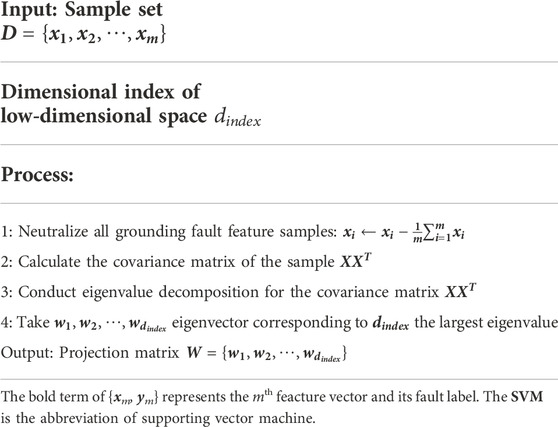
TABLE 1. PCA algorithm principle and pseudo-code.

In combination with the principal component analysis method, the dimensionality reduction engineering construction of grounding fault features in Section 1.2 is carried out. There is an independent and unrelated eigenvalue distribution in the new space after construction. After considering the principle of the “90%” value space, Figure 3 depicts the selection of the top 10 eigenvalues, and the cumulative ratio of features accounts for 91.37%. Therefore, the initial structure with 1,536-dimension load feature engineering can be optimized and reduced to 12 dimensions, and the space compression rate can reach as high as 99.21%.

FIGURE 3

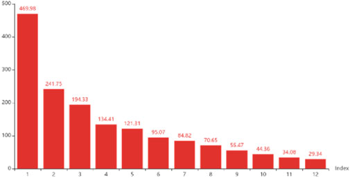
FIGURE 3. Distribution of eigenvalues of single-phase grounding faults after dimensionality reduction using the PCA method.

3.3 AdaBoost classification model

Since for every set of feature vectors, its classification result is provided; obviously, this issue belongs to the supervised learning field. In machine learning, logistic regression, support vector machine, K-neighbor proximity, and decision tree, as well as integration-based learners, such as AdaBoost, XGBoost, and LightGBM, are typical technologies used (Wu and Hiroshi, 2014; Dahlan, 2018; Pan et al., 2020). Compared with a single classifier (also known as a “weak learner”), integrated learning combined with multiple learners can often obtain significantly better generalization performance than a single learner. As demonstrated by many practical applications, however, AdaBoost presents better convergence performance, consumes less time, and occupies lower memory resources. As such, this section will mainly focus on extending this algorithm to the online model in identifying single-phase earth faults.

Bagging and boosting methods focus on sample sampling and parallel learning, and error sample relearning and reinforcement of the base learner, respectively. It is obvious that the latter has more advantages. In view of this, based on optimization of the fault feature set by dimensionality reduction of the PCA method, this section will build a single-phase grounding fault classification model combined with Boosting’s AdaBoost method. Of which, the base learner of the AdaBoost method primarily utilizes SVM in order to enhance the robustness of the classification effect of the model.

Furthermore, the pseudo-code of the principle of constructing the grounding fault classification model combined with the AdaBoost method is shown in Figure 2.

3.4 The flowchart of the proposed identification model

Combined with Sections 2–3, the proposed single-phase earth fault identification model based on AdaBoost is detailed in Figure 4. As seen from Figure 4, it mainly includes five key steps: data preprocessing, construct feature, feature engineering, build AdaBoost-based identification model, and optimize hyperparameter. Particularly, data preprocessing used for extracting zero-sequence voltage and zero-sequence current is first conducted. Second, Step B constructs fault features via current mainstream algorithms in addition to the proposed angle-conversion model. Next, feature engineering is explored according to PCA-based algorithm to select the best and most sensitive features. Subsequently, a custom-designed single-phase earth ground fault identification model is put forward, where an AdaBoost-based model is conducted as an example and numerically compared in detail.

FIGURE 4

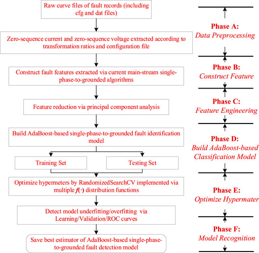
FIGURE 4. AdaBoost-based single-phase earth ground fault identification model.

4 Numerical studies

In order to verify the effectiveness of the method proposed in this article, a single-phase grounding fault feature set is constructed by combining the two dimensions of true waveform and simulation modeling. Of these, the distribution network model based on PSCAD, as shown in Figure A1, and the selected Mianyang true test waveform are established. The single-phase grounding fault with variable parameters such as arc suppression coil grounding system and ungrounded system under different load levels, fault initial phase angle, and transitional resistance, along with normal operation tests of the system, such as non-synchronization closing, magnetizing inrush current, and non-synchronization load commissioning and decommissioning, has been taken into consideration.

FIGURE A1

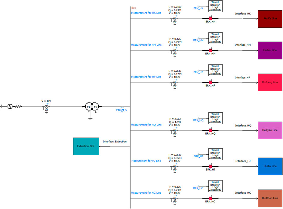
FIGURE A1. Single-phase grounding fault simulation system of a distribution network based on PSCAD.

The result is that the number of single-phase grounding fault samples and anti-interference samples is, respectively, 108 and 27, equating to a ratio of nearly 6:1. In combination with up-sampling technology, the ratio of the number of fault samples and non-fault samples will be adjusted to 1:1, and the total number of samples will be 216. In addition, the initial fault feature dimension is 1,536 dimensions. After dimensionality reduction by the PCA method in Section 2.2, the dimension of the eigenvector will be adjusted to 12 dimensions, with a compression rate as high as 99.21%.

4.1 Statistical analysis of single-phase grounding fault features

In combination with Section 1.2, the $\mathcal{M}=\left[U_p^{amp},{∆U}_p^{amp},U_p^{theta},I_p^{amp},{∆I}_p^{amp},I_p^{theta}\right]$ of single-phase grounding fault feature engineering can be constructed directly, but there is a lack of the boost method to learn the process mechanism between feature engineering and target. In this regard, the following will take $3U_0$ of zero-sequence voltage amplitude and $3I_0$ of zero-sequence current amplitude of single-phase grounding fault under systems of arc suppression coils being grounded and ungrounded as examples to provide their distribution statistical curves, as shown in Figures 5, 6, respectively.

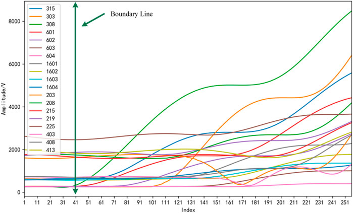
FIGURE 5

FIGURE 5. $\mathit{3}{U}_{\mathit{0}}$ amplitude change curve when a single-phase grounding fault occurs in arc suppression coil grounded and ungrounded systems.

FIGURE 6

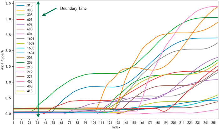
FIGURE 6. 3I0 amplitude change curve when a single-phase grounding fault occurs in arc suppression coil grounded and ungrounded systems.

It can be seen from Figures 5, 6 that no matter whether the system is grounded or not, there are obvious demarcations for the zero-sequence voltage and zero-sequence current of the system, which correspond to before and after the fault. In addition, after demarcation, $\mathit{3}{\mathit{U}}_{\mathit{0}}$ and $\mathit{3}{\mathit{I}}_{\mathit{0}}$ show a trend of gradual increase and deterioration. The two features clearly illustrate the necessity and importance of adopting $\mathit{3}{\mathit{U}}_{\mathit{0}}$ and $\mathit{3}{\mathit{I}}_{\mathit{0}}$ to build feature engineering for grounding faults, and they can provide favorable learning features for the AdaBoost method, thus guiding it to build a reasonable single-phase grounding fault classification learning model.

4.2 AdaBoost accuracy rate of the AdaBoost grounding fault classification model

For the simulation test and true waveform fault set, after adopting the single-phase grounding fault classification model constructed using AdaBoost algorithm in Table 2, the confusion matrix (Shu et al., 2019) of fault and non-fault samples, including the training set and test set, can be obtained, as shown in Table 3.

TABLE 2

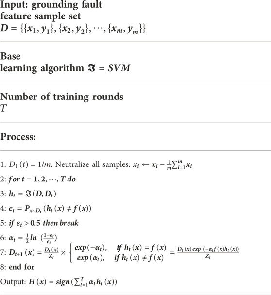
TABLE 2. Pseudo-code of the ground fault classification learning model based on AdaBoost proposed by Shu et al. (2019).

TABLE 3

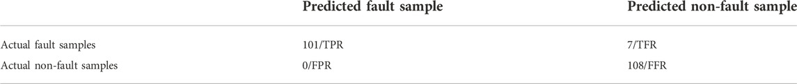
TABLE 3. AdaBoost confusion matrix.

In Table 3, indicators TPR, TFR, FPR, and FFR represent the true-positive rate, true-false rate, false-positive rate, and false rate, respectively (Shu et al., 2019). According to the confusion matrix in Table 3, there are 101 correct predictions of fault cases, up to 93.52% of the total, while the prediction accuracy of non-fault examples is 100%, with all predictions divided correctly. After analyzing the seven waveforms being incorrectly divided for fault examples, the errors are all attributed to one type of reason, namely, the grounding fault of ultra-high resistance Rd. Data from a real test in Mianyang is taken as an example: single-phase grounding fault under the mixed medium of branches and leaves on the cement ground through 50 cm conductor; line voltages ${\mathit{U}}_{\mathit{a}\mathit{b}}$, ${\mathit{U}}_{\mathit{b}\mathit{c}}$, ${\mathit{U}}_{\mathit{0}}$, ${\mathit{I}}_{\mathit{a}}$, ${\mathit{I}}_{\mathit{b}}$, ${\mathit{I}}_{\mathit{c}}$, and ${\mathit{I}}_{\mathit{0}}$ of corresponding line are shown in Figure 7.

FIGURE 7

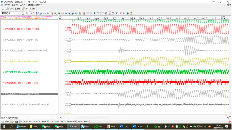
FIGURE 7. Single-phase grounding fault under the mixed medium of branches and leaves on the cement ground through a 50-cm conductor.

According to Figure 6, when the system is in normal operation, the voltage imbalance is nearly 3%. As far as the zero-sequence voltage change curve is concerned, the fault belongs to a long-term gradual fault, and the change of zero-sequence voltage is also a process of gradual deterioration and increase. At the first fault moment, the transitional resistance reaches as high as 27k, and $\mathit{3}{\mathit{U}}_{\mathit{0}}$ and $\mathit{3}{\mathit{I}}_{\mathit{0}}$ change slightly. Most algorithms are likely to include this into the category of zero-sequence voltage fluctuation caused by non-synchronization load of system commissioning and decommissioning. However, in the second fault after 612 ms, the sudden trend changing of zero-sequence voltage and the obvious characteristics of opposite polarity of $\mathit{3}{\mathit{U}}_{\mathit{0}}$ and $\mathit{3}{\mathit{I}}_{\mathit{0}}$ can obviously be judged as a single-phase grounding fault for most algorithms. In terms of the latter, the single-phase grounding fault classification model based on AdaBoost constructed in this article can also study and judge the grounding fault.

In addition, after further analyzing the waveform, it is found that the reasons for the poor effect of most algorithms also relate to two aspects. The first aspect is the algorithm level. Looking at the waveform, even 100 ms after the fault has occurred, in combination with the obvious opposite direction characteristics of zero-sequence voltage and zero-sequence current, the head half-wave method and steady-state method can still identify the fault. For the parameter method, the zero voltage change trend is not obvious in the middle of the fault, which can easily lead to the failure of the parameter method. The second aspect is the response speed. From the perspective of fault form, this is a long-time gradual fault, and the interval between the salient features of the two faults is 618 ms. If the fault can be identified only in the second salient feature, it is likely that the hidden danger of mountain fire will occur due to the burning of dry leaves caused by the previous fault, and the best rescue opportunity will be missed.

4.3 Performance of the AdaBoost single-phase grounding fault classification model

In order to help build the algorithm and give full play to its practical application, the performance of the proposed AdaBoost single-phase grounding fault classification model will be verified from the dimensions of the learning curve and ROC curve. In order to understand the intuitive evaluation of the performance of the classification model from the perspective of the two types of curves, the definitions of the two types of curves will be described first.

4.3.1 Learning curve

The learning curve is the score change curve of sizes and models of different training sets on the training set and verification set, that is, the number of samples is taken as the abscissa, and the scores on the training and cross-validation sets (such as accuracy) are taken as the ordinate. A learning curve can help us judge the current state of the model: overfitting/high variance or underfitting/high-bias. Figure 8 shows the learning curve for measuring the degree of overfitting or underfitting of the model. The high variance emphasizes that the generalization ability of the model is not ideal when applied to the test set, while the high-bias characterization model lacks the deep mining of feature engineering.

FIGURE 8

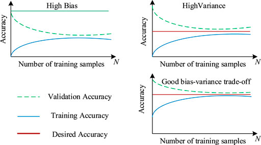
FIGURE 8. Learning curve used for assessing model overfitting/underfitting.

4.3.2 Receiver operating characteristic curve

The receiver operating characteristic curve (ROC curve in short) is also known as the sensitivity curve. The reason for such a name is that the points on the curve reflect the same sensitivity. They are all responses to the same signal stimulus, but the results have been obtained under several different criteria. The general outline of the ROC curve is shown in Figure 9.

FIGURE 9

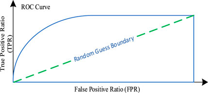
FIGURE 9. ROC curve to measure the pros and cons of model classification performance.

In Figure 9, the receiver operating characteristic curve is a coordinate diagram composed of false alarm probability as the horizontal axis and hit probability as the vertical axis. The curve drawn reflects the different results obtained by the subjects under specific stimulus conditions due to different judgment criteria. The ROC curve emphasizes the balance between TPR and FPR, which can effectively avoid the influence of differentiation of different judgment criteria.

Combined with the classification characteristics of single-phase grounding faults, the higher the proportion TPR of the samples predicted to be positive and actually positive in Figure 8 in all positive samples, the lower the proportion FPR of the samples predicted to be positive but actually negative in all negative samples; or the higher the area of the blue closed area constructed by points (FPR and TPR) (random guess: the area of the closed graph is 0.5), the better the performance of the fault classification model.

Furthermore, the learning curve and ROC curve based on the AdaBoost single-phase grounding fault classification model are given in Figures 10, 11, respectively.

FIGURE 10

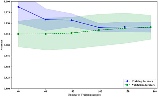
FIGURE 10. Application of the AdaBoost ground fault classification model learning curve.

FIGURE 11

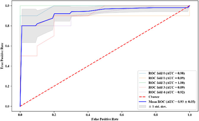
FIGURE 11. ROC curve of the AdaBoost ground fault classification model.

It can be seen from Figure 10 that with the increase of the number of training samples, the classification accuracy of the training set and the verification set gradually trend toward sameness, and the classification accuracy of the verification set gradually increases. The generalization ability of the characterization model applied to the unknown fault set is strong, but the improvement of this ability comes at the expense of a certain level of weakening of the training effect of the training set. Therefore, the performance of the classification model constructed by the machine learning method represented by AdaBoost depends on the compromise of training and verification effects, and it is also the balance between high-bias and high variance of the classification model.

With regard to Figure 10, it can be seen that under the premise of cross validation of five copies for the training set, the AUC of each corresponding ROC curve is 0.98, 0.89, 1.00, 0.89, and 0.92, respectively, which are far higher than 0.5 of random guess, and the overall average AUC /standard deviation of AUC is 0.93 and ±0.05. A small standard deviation indicates that the training effect of the model is relatively stable. Moreover, comparative studies between the proposed and the other two methods are also conducted, namely, logistic regression (LR) and K-neighbor (KN), as shown in Table 4. As seen from Table 4, both the accuracy and AUC indicators of the model constructed in this work are superior, which fully demonstrates the validity and the high value in engineering practice.

TABLE 4

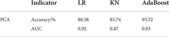
TABLE 4. Identification effects of six models based on machine learning under PCA-based feature engineering.

In general, the AdaBoost single-phase grounding fault classification model established in this article can better adapt to the differential selection of different judgment criteria under specific stimulus conditions, the overall performance is more stable, and the robust performance is better.

5 Conclusion

This article discusses the classification research of machine learning algorithm jointly driven by both physical model and fault data in single-phase earth ground fault identification and constructs a single-phase grounding fault classification model based on AdaBoost. For PSCAD simulation model and fault and non-fault examples under the true waveform test, the classification accuracy of the model is 93.52%. Second, in conjunction with up-sampling technology, PCA dimensionality reduction technology, learning curve, and ROC curve, the construction of feature engineering, dimensionality reduction optimization, and model performance evaluation are achieved, respectively. Among them, after PCA dimensionality reduction technology is adopted, feature engineering can be transformed into the feature space represented by a 12-dimension vector with a space compression rate as high as 99.21%. The training effect of the training set and verification set in the learning curve tends to be 0.93 as a whole, and the average AUC under cross verification also reaches nearly 0.93, which mutually confirms the highly accurate training effect of the proposed AdaBoost model and the identification and generalization ability of grounding faults under strong interference and bad working conditions.

Data availability statement

The raw data supporting the conclusion of this article will be made available by the authors, without undue reservation.

Author contributions

All authors listed have made a substantial, direct, and intellectual contribution to the work and approved it for publication.

Funding

This work was supported by the State Grid Sichuan Supply Company Science Project under grant no. 52199720002T.

Conflict of interest

HY, ZW, and ZQ were employed by Nari Technology Nanjing Control Systems Co., Ltd.

The remaining authors declare that the research was conducted in the absence of any commercial or financial relationships that could be construed as a potential conflict of interest.

The authors declare that this study received funding from State Grid Sichuan Supply Company Science Project. The funder had the following involvement in the study: collection, analysis, interpretation of data.

Publisher’s note

All claims expressed in this article are solely those of the authors and do not necessarily represent those of their affiliated organizations, or those of the publisher, the editors, and the reviewers. Any product that may be evaluated in this article, or claim that may be made by its manufacturer, is not guaranteed or endorsed by the publisher.

References

An, D., Chen, T., Li, J., Yao, K., Zhang, H., and Wang, H. (2020). Design of a small current grounding line selection device based on a half-wave Fourier algorithm. [J], Power Syst. Prot. Control 48 (09), 157–163.

Google Scholar

Ai, B., Zhang, R., and Li, Y. (2009). Overview of line selection technology for small current earth fault. North China Electric Power, Beijing.

Google Scholar

Cui, T., Dong, X., Zhiqian, B., and Juszczyk, A. (2011). Hilbert-transform-based transient/intermittent earth fault detection in noneffectively grounded distribution systems. IEEE Trans. Power Deliv. 26 (1), 143–151. doi:10.1109/tpwrd.2010.2068578

CrossRef Full Text | Google Scholar

Dahlan, R. (2018). “AdaBoost noise estimator for subspace based speech enhancement[C],” in 2018 international conference on computer, Control, informatics and its applications (IC3INA), 110–113.

Google Scholar

Gautam, S., and Brahma, S. M. (2012). Detection of high impedance fault in power distribution systems using mathematical morphology. IEEE Trans. Power Syst. 28 (2), 1226–1234 Aug. doi:10.1109/tpwrs.2012.2215630

CrossRef Full Text | Google Scholar

Ghaderi, A., Ginn, H. L., and Mohammadpour, H. A. (2017). High impedance fault detection: A review. Electr. Power Syst. Res. 143, 376–388. doi:10.1016/j.epsr.2016.10.021

CrossRef Full Text | Google Scholar

He, L., Shi, C., Yan, Z., Cui, J., and Zhang, B. (2017). A fault location method for small current grounded systems based on the relative entropy of generalized S-transform energy[J]. Trans. Chin. Soc. Electr. Eng. 32 (08), 274–280.

Google Scholar

Jiale, S., Kang, X., and Song, G. (2007). etc. A preliminary study on the principle of relay protection based on parameter identification[J]. J. Electr. Power Syst. Automation 19 (1), 14–20.

Google Scholar

Li, X. (2017). Line selection method of small current Earth fault based on three lines display. Electr. Eng. 4, 6–7.

Google Scholar

Lishan, W., Jia, W., and Jiao, Y. (2020). Single-phase fault line selection scheme of a distribution system based on fifth harmonic and admittance asymmertry[J]. Power Syst. Prot. control 48 (15), 77–83.

Google Scholar

Liu, W., Xu, B., Liu, Y., Wang, A., and Chen, H. (2018). Small current grounding fault demarcation method based on transient current[J]. Automation Electr. Power Syst. 42 (24), 157–162+202.

Google Scholar

Pan, Z., Fang, S., and Wang, H. (2020). LightGBM technique and differential evolution algorithm-based multi-objective optimization design of DS-APMM. IEEE Trans. Energy Convers. 36 (1), 441–455. doi:10.1109/tec.2020.3009480

CrossRef Full Text | Google Scholar

Shu, H., Li, Y., Tian, X., and Yi, F. (2019). Distribution network fault line selection based on correlation analysis of cross-overlap differential transformation[J]. Automation Electr. Power Syst. 43 (06), 137–144+ 176.

Google Scholar

Song, G., Guang, L., and Yu, Y. (2011). Location of single-phase grounding fault section in distribution network based on sudden changes in phase current [J]. Automation Electr. Power Syst. 35 (21), 84–90.

Google Scholar

Wang, W., Cheng, L., and Fan, Y. (2021). Earth fault identification method for distribution station independent of zero sequence voltage. Automation Electr. Power Syst. 45 (9), 122–129.

Google Scholar

Wu, S., and Hiroshi, N. (2014). Parameterized AdaBoost: Introducing a parameter to speed up the training of real AdaBoost. IEEE Signal Process. Lett. 21. (6), 687–691. doi:10.1109/lsp.2014.2313570

CrossRef Full Text | Google Scholar

Xu, B., Xue, Y., and Li, T. (2005). Overview of line selection technology for small current Earth fault. Electr. Equip. 4, 1–7.

Google Scholar

Xue, Y., Li, J., and Xu, B. (2015). The transient equivalent circuit and transient analysis of the small current grounding fault of the neutral point through the arc suppression coil grounding system[J]. Proc. Chin. Soc. Electr. Eng. 35 (22), 5703–5714.

Google Scholar

Xue, Y., Zuren, F., Xu, B., Chen, Y., and Jing, L. (2003). Research on low current grounding line selection based on transient zero sequence current comparison [J]. Automation Electr. Power Syst. 4 (09), 48–53.

Google Scholar

Yao, H., and Cao, M. (2009). Resonant grounding of power system [M]. Beijing: China Electric Power Press.

Google Scholar

Zeng, X., Wang, Y., Jian, L., and Xiong, T. (2012). New principles of fault arc suppression and feeder protection based on flexible grounding control of distribution network[J]. Proc. Chin. Soc. Electr. Eng. 32 (16), 137–143.

Google Scholar

Zhang, B., and Yin, X. (2011). Power system relay protection [M]. Background: China Electric Power Press.

Google Scholar

Zhou, Z. (2016). Machine learning [M]. Beijing: Tsinghua University Press.

Google Scholar

Zhu, L. (2011). Research on single-phase short-circuit fault and its protection of low resistance grounding system in 10kV distribution network [D]. Changsha: Hunan University.

Google Scholar