Parameter Identification of Electromechanical Oscillation Mode in Power Systems Driven by Data: A Quasi-Real-Time Method Based on Randomized-DMD-Multilayer Artificial Neural Networks

With the increase in the power system scale, the identification of electromechanical oscillation mode parameters by traditional numerical methods can no longer meet the requirements of complete real-time analysis. Therefore, a method based on machine learning (multilayer artificial neural networks) is proposed to identify the electromechanical oscillation mode parameters of the power system. This method can take the monitorable variables of the WAMS as the input of the model and the key characteristic information such as frequency and damping ratio as the output. After processing the input and output data with randomized dynamic mode decomposition (randomized-DMD), their mapping relationship can be analyzed by using the multilayer neuron architecture. The simulation results of the 4-generator 2-area system and the IEEE 16-generator 5-area system show that this method can accurately calculate the key characteristic parameters of the system without considering the change in the control parameters and after the offline training of historical data, which shows higher accuracy, stronger robustness, and sensitive online tracking ability.

1 Introduction

With the rapid development of smart grids and ultra-high voltage AC/DC power transmission, the dimension of the dynamic model of a power system has gradually increased in recent years. With the regional interconnection of the power system and the accessibility of various components, the stability analysis of a small disturbance in the power system is carried out using with a large-scale differential-algebraic system (Shair et al., 2021). One of the challenges is how to analyze the key oscillation mode parameters of a large-scale power system. The fluctuation and time variability of the power system’s operation state are enhanced. This feature requires the small disturbance safety and stability analysis to be completed in a shorter time scale to achieve the purpose of real-time analysis. In addition, the changeable and uncertain operating state of the system generates the demand for small disturbance stability security warnings. To ensure the security and stability of the system, it is necessary to predict the running state of the system and evaluate the development direction of the stability of small disturbances on the premise of taking volatility into account. Considering the characteristics of time variability and volatility, it is a new challenge to evaluate the stability of small disturbances in real time. With the popularity of the wide area measurement system (WAMS), which is based on the phasor measurement unit (PMU), the analysis method of random response signals is based on ambient excitation that came into being. A large number of WAMS-measured data can be recorded during the normal operation of the power system. Due to random disturbances such as random small fluctuations in load and intermittent output of new energy, there is a random response of small fluctuations at any time in the power grid.

1.1 Numerical Analysis Method

Pierre et al. (1997) verified the feasibility of using random response signals to extract low-frequency oscillation mode parameters of the system for the first time, laying a solid theoretical foundation for the subsequent oscillation mode identification based on random response signals. In recent years, a large number of identification methods for random response signals based on wide-area measurement have emerged (Khalilinia et al., 2015; Khalilinia and Venkatasubramanian, 2017).

There are two main categories of random data-driven low-frequency oscillation mode parameter extraction methods: the block processing method and recursive analysis. The block processing method estimates the oscillation mode parameters of the system that is based on the sampled measured data of a certain length of the analysis window. This included the use of Yule-Walker equations (Pierre et al., 1997), modified Yule-Walker equations (Wies et al., 2003), and extended modified autoregressive moving average (ARMA) equations estimated by Yule-Walker (Wies, 1999), detecting the main oscillation modes in ambient data. To improve the estimation quality, Anderson et al. (2005) designed a confidence interval mode estimation based on bootstrap. Recursive analysis updates the mode characteristic information of that moment by using the updated data and the mode identification results of the previous data after acquiring the new sample measurement data. To suppress outliers and missing data in ARMA-based main mode estimation, a robust recursive least squares (RRLS) ARMA model was established to detect main modes from ambient data (Zhou et al., 2007). Aiming at the problem that the ARMA model based on RRLS cannot process atypical data of power systems, an autoregressive moving average exogenous (ARMAX) model based on regularized RRLS (R3LS) was proposed, which considered both typical and atypical measurement data (Zhou et al., 2008). ARMA model parameters were calculated based on the recursive prediction error method (RPEM), and then the mode parameters of the system were estimated (Dosiek et al., 2013). An online tracking method of low-frequency oscillation mode parameters based on recursive adaptive random subspace was proposed (Nezam Sarmadi and Venkatasubramanian, 2014).

1.2 Artificial Intelligence Method

With the large-scale access of a high proportion of wind power, photovoltaics, and other new energy sources, the power grid presents characteristics such as greater time variability and volatility, which requires the safety and stability assessment of small disturbances in operation scheduling to be completed within a shorter time scale to achieve the purpose of real-time analysis in the process of system operation. The stability assessment method based on the deterministic linear model and data is widely used in engineering. However, the dimension of the dynamic mathematical model of the large-scale system is very large with high computational complexity, so it is difficult to meet real-time requirements. In recent years, machine learning has been applied to the power system. It can obtain results quickly without building a complex mathematical model. For stability assessment of small disturbances, artificial intelligence can be combined with traditional methods to achieve real-time performance. Artificial intelligence has some applications in power system oscillation (Chan and Nopphawan, 2020; Shi et al., 2020) and damping control (Ravikumar and Govindarasu, 2020).

The dimension of the dynamic mathematical model of a large-scale system is huge (Li et al., 2016), and to calculate all eigenvalues, numerical methods such as orthogonal trigonometric decomposition (QR/BR) (Ma et al., 2006) can no longer adapt to small disturbance stability analysis. For calculating a part of the eigenvalues, numerical methods such as the Arnoldi method (Angelidis and Semlyen, 1996) also have high computational complexity, and it is difficult to meet the real-time requirements of computing speed even if parallel computing is adopted.

The traditional small disturbance stability assessment method has a low computational complexity in directly analyzing the measured data. With the rapid development of artificial intelligence, methods based on machine learning in power system transient stability assessment have a lot of applications, such as offline time-domain simulation and the study of the sample set to extract the unknown mapping function relations, which are often used for system transient stability analysis. The machine learning method accepts samples without accepting the limitation of the system model. Once the functional relation is determined, stability analysis for the new operation mode can be very fast with intuitively featured results. Thus, it becomes a very attractive method for safety assessment.

There are some methods of small disturbance stability analysis that are data-driven (You et al., 2020; Liu et al., 2021). Taking the infinite size of a single machine as an example, Lima and Alden (1994) used a three-layer neural network to classify small disturbance stability and instability, achieving an accuracy rate of more than 99%. Each piece of the node information of the system was used as the input variable for the selection of PCA (Teeuwsen et al., 2003); according to the spatial distribution, the system’s key characteristic value can be grouped by symbols; different neural networks for the various key oscillation modal simulation systems were modeled, which realized the accurate characteristics’ category classification.

Another method is based on the support vector machine (SVM) and its variants, Mohammadi and Gharehpetian (2009) used various nodes of active power, reactive power, and voltage as input using the decision tree method for input variable selection. The SVM method can identify small disturbance stability or instability. The New England 39 node system for small disturbance stability classification has been verified to obtain good results. In addition, Mohammadi and Gharehpetian (2009) improved to adopt a multiclassification method (Han-SVM). By changing the load power from 50% to 200%, the corresponding training set and test set were obtained. The stable state of small disturbances could be classified after training (Mohammadi and Gharehpetian, 2008). To improve the training speed, an improved SVM method, the BVM (ball vector machine), was adopted for modeling by Mohammadi et al. (2010), and the small disturbance stability was divided into four categories. The training time was significantly shorter than that of the SVM. However, the SVM-based method is difficult to be applied to large-scale interconnected power grids because the kernel function used by the SVM is difficult for large-scale interconnection network design. Moreover, SVMs use one-time optimization to solve the training set data. Since the training set data of a large-scale interconnected power grid is large, the calculation time is very long.

Since the small disturbance stability analysis methods based on artificial intelligence are all classification methods, that is, the analysis of small interference stability or small disturbance instability fails to provide an early warning for the normal operation of the system, in this paper, a multilayer artificial neural network is applied for parameter identification of the electromechanical oscillation mode of the power system, and the potentially weakly damped mode in the system is found under the normal operation state.

We can monitor the WAMS variables (generator speed, power angle, and active power) and arrange them in two-dimensional matrix forms as the input and construct the structure of the multilayer ANN; after training, a large number of historical data on the system critical oscillation characteristics such as frequency and damping ratio of the real-time computation model were established, and this method has achieved a good effect on the 4-generator 2-area system and the 16-generator 5-area system.

The applications of the randomized-dynamic-mode-decomposition-multilayer artificial neural network (R-M-ANN) model in the electrical power system oscillation mode parameter identification are presented in this paper. The WAMS system can monitor the variables (generator speed, power angle, and active power) arranged in two-dimensional matrix forms as the input; the construction of the structure of the R-M-ANN has the advantages of the R-M-ANN’s feature extraction without considering the system control equipment under the condition of parameter change; after a lot of historical data training, a key oscillation information system under the random response data real-time vibration model is established, and the method has achieved a better effect on the case study. The rest of this study is structured as follows: Section 2 provides a brief review of the multilayer ANN. Section 3 provides the process of electromechanical oscillation identification using the randomized-DMD-multilayer ANN model. Section 4 shows the case studies for the 4-generator 2-area system and the IEEE 16-generator 5-area system. Section 5 presents the concluding remarks.

2 Brief Review of Multilayer ANN

The core idea of the R-M-ANN is to build a model of a class of algorithms based on neuroscience. When given input data, neurons can transmit information layer by layer (Zupan, 1994), and neurons can be activated if the signal is strong enough. The data travel through the network until the final step is reached—the output layer—from which we derive our predictions. These predictions can then be compared with the expected output to calculate the predicted errors, which the network uses to learn and improve future predictions (Gershenson, 2003). The multilayer ANN has nonlinear properties. This helps the network learn any complex relationship between the input and output (Kenji, 2011). A multilayer artificial neural network consists of several neurons, including three types of layers (Teoh et al., 2006), shown in Figure 1. The common learning algorithm of artificial neural networks is the backpropagation algorithm. The weights of a neural network are updated through this backpropagation algorithm by finding the gradients. Error is often calculated by the mean square error function, which is returned to the neural network, and the weight is modified accordingly (Rai et al., 2011). This process is called backpropagation. Through this algorithm, the artificial neural network can adjust the ownership weight and reach the set threshold through multiple adjustments to complete the training of the neural network (Goh, 1995).

FIGURE 1

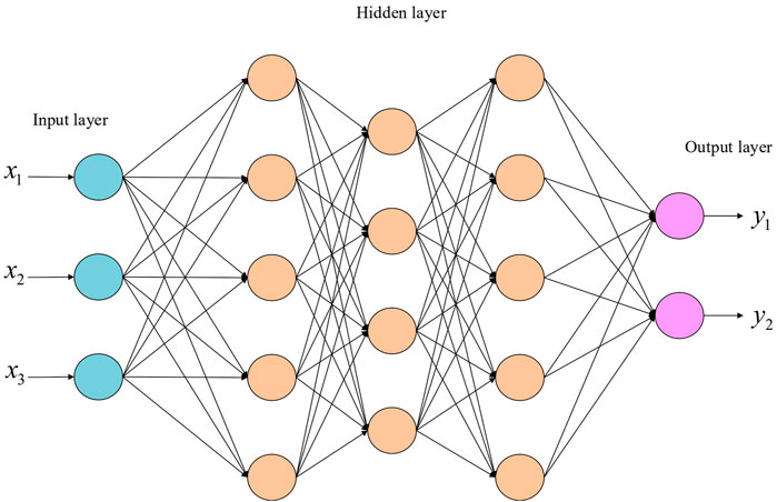
FIGURE 1. Multilayer artificial neural network.

3 Electromechanical Oscillation Identification Based on Randomized-DMD-Multilayer ANN Model

The dynamic mode decomposition (DMD) algorithm is a numerical decomposition method; under certain conditions, it is based on the modal decomposition of the Koopman operator (Tu et al., 2014).

Supposing the kth sampling point of the state variable at $t_k$ is $\mathrm{\Delta }{\underset{¯}{x}}_k=\mathrm{\Delta }\underset{¯}{x}\left(t_k\right)$. The snapshot data are a moving window, including the latest sampling point in the window interval. The snapshot data can be described by the following matrix:

$X^{\left(m-1\right)}=\left[\mathrm{\Delta }{\underset{¯}{x}}_0,\mathrm{\Delta }{\underset{¯}{x}}_1,\dots ,\mathrm{\Delta }{\underset{¯}{x}}_{m-1}\right]\in R^{m\times n}(1)$

$X^{\left(m\right)}=\left[\mathrm{\Delta }{\underset{¯}{x}}_1,\mathrm{\Delta }{\underset{¯}{x}}_2\dots ,\mathrm{\Delta }{\underset{¯}{x}}_m\right]\in R^{m\times n}(2)$

We have

$X^{\left(m\right)}=A{X}^{\left(m-1\right)}(3)$

$A=X^{\left(m\right)}{X}^{{\left(m-1\right)}^{†}}(4)$

where $†$ represents the Moore–Penrose pseudoinverse. Therefore, we can obtain that if a system is linear (or approximately linear in reality), we can recover the system through the state’s “trajectory data”, which are

$\left[\mathrm{\Delta }{\underset{¯}{x}}_1,\mathrm{\Delta }{\underset{¯}{x}}_2\dots ,\mathrm{\Delta }{\underset{¯}{x}}_m\right](5)$

Because of the huge high dimensionality of the data, the $X^{\left(m\right)}$ matrix is $m\times n$, but $n\gg 1$. Therefore, it is difficult to calculate the eigenvalues and eigenvectors of $X^{\left(m\right)}{X}^{{\left(m-1\right)}^{†}}$, which need to be decomposed by the DMD method.

First, the r order approximately truncated singular value decomposition (SVD) of the original data matrix $X^{\left(m-1\right)}$ is calculated using Eq. 6. Keeping only the first r order of the SVD process can decrease the calculation cost and ensure accuracy.

$X^{\left(m-1\right)}=U_r{\text{Σ}}_r{V}_r^T(6)$

A matrix $\tilde{A}=U_r^T{X}^{\left(m\right)}{V}_r{\text{Σ}}_r^{-1}$ is set, and then the eigendecomposition of matrix $\tilde{A}$ is calculated, which means calculating $\tilde{\omega }$ and $\lambda$ using the formula $\tilde{A}\tilde{\omega }=\lambda \tilde{\omega }$.

The DMD mode corresponding to the DMD eigenvalue $\lambda$ is then given by

$\widehat{\phi }=U_{r}w(7)$

Then the return to the dynamic modes and corresponding eigenvalues $\lambda$ can be calculated by the following formula:

$\omega ={\lambda }^{-1}{X}^{\left(m\right)}{V}_r{\text{Σ}}_r^{-1}\tilde{\omega }(8)$

It can be seen that the SVD algorithm is the main part of the DMD algorithm, so the improvement of the SVD algorithm will greatly improve the DMD algorithm. In the next section, we will introduce an improved DMD algorithm.

3.1 Randomized Dynamic Mode Decomposition

Randomized algorithms have various applications, which have more advantages in solving the linear least squares problems and low-rank matrix approximation (Drineas and Mahoney, 2016). In this paper, we can multiply matrix A with a random matrix on its right side or left side to identify the subspace capturing the dominant actions of matrix A and then obtain the subspace’s orthonormal basis matrix Q. We can further provide the approximate truncated SVD after computing a low-rank approximation of matrix A with matrix Q. This method can facilitate the results of near-optimal decompositions of matrix A because the dimension of the subspace is much smaller than that of range (A).

We claim four inputs for randomized-SVD, which are $A\in R^{m\times n}$, rank parameter k, power parameter p, and oversampling parameter s. Furthermore, the three outputs presented in the randomized-SVD are $U_r\in R^{m\times m}$, ${\text{Σ}}_r\in R^{m\times n}$, and $V_r\in R^{n\times n}$.

A Gaussian-independent and identically distributed (i.i.d) matrix $\text{Ω}$ is set as shown below:

$\text{Ω}=\text{randn}\left(n,k+s\right)(9)$

In order to obtain better accuracy, s could enable $\text{Ω}$ with more than k number of columns, which is a small integer such as 5 or 10.

Furthermore, $\text{Ω}$ can be replaced by other kinds of random matrices to decrease the computational cost $A\text{Ω}$, but they also bring some sacrifice on accuracy.

With the subspace’s orthogonal basis matrix Q, A and $\omega$ are used to compute the subspace orthogonal basis matrix Q, which is

$Q=orth\left(A\text{Ω}\right)(10)$

We have the approximation $A\approx QB=Q{Q}^{T}A$. Then, performing the economic SVD on the $\left(k+s\right)\times n$ matrix B, we obtain the approximate truncated SVD of A. To improve the accuracy of the $QB$ approximation, a technique called the power iteration (PI) scheme can be applied; setting i = 1, 2…, p, the iteration is carried out with

$G=orth\left(A^T\text{Q}\right)(11)$

$Q=orth\left(A\text{G}\right)(12)$

where the equation of $orth$ is used to alleviate the round-off error in the floating-point computation and achieved by QR factorization. Then it forms as

$B=orth\left(Q^T\text{A}\right)(13)$

which yields a low-rank factorization $\text{A}\approx Q{Q}^{T}A$. When there are few columns in Q, it is efficient to construct B easily and compute its SVD rapidly.

It is based on the fact that matrix ${\left(A{A}^T\right)}^{p}A$ has exactly the same singular vectors as A, but its singular value decays more quickly. Thus, performing a randomized $Q{Q}^{T}A$ procedure on ${\left(A{A}^T\right)}^{p}A$ can achieve better accuracy.

U can be calculated through singular value decomposition (SVD) of the original small matrix $B$, which is

$\left[U_r,{\text{Σ}}_r,V_r^T\right]=svd\left(B\right)(14)$

Then the first-k columns of $QU$ are returned: the first-k matrix of $\text{Σ}$ and first-k columns of $V$. Eq. 6 can be replaced by Eq. 14 to continue the DMD process.

We can often avoid forming B explicitly by means of a subtler technique. In some cases, it is not even necessary to revisit the input matrix A during matrix approximation framework. This observation can allow us to develop a single pass method to look at each entry of A only once.

Using the randomized-DMD algorithm, some descriptions are presented to provide oscillation temporal characteristics (oscillation frequency $f_i$ and damping ratio ${\sigma }_i$) from the measurement data. For example, we extract the eigenvalues ${\eta }_i$, which are transformed from the measured data into continuous system mode expression.

${\eta }_i=\log {\lambda }_i/\mathrm{\Delta }t(15)$

Then the frequency and damping ratio of the ith mode are calculated, which are

$f_i=Imag\left\{{\eta }_i\right\}/2\pi (16)$

${\sigma }_i=Re\left\{{\eta }_i\right\}(17)$

The mode matrix is defined as

$\varphi =\left[{\phi }_1,\dots ,{\phi }_n\right](18)$

which is the corresponding dynamic mode ${\varphi }_i$.

3.2 Multilayer ANN Model

In the traditional small-signal stability analysis method, each dynamic element of the system needs to be linearized at the operating point, and the state matrix is calculated as an input to further analyze the eigenvalues. However, the calculation of the state matrix is time-consuming for large systems. To achieve stable real-time analysis with small disturbances, it is obviously impossible to use the state matrix as the input.

At present, the WAMS is widely being used in power systems above the provincial level (Phadke, 2002) and is becoming an important data platform for dynamic monitoring and control of wide-area power systems (De La Ree et al., 2010). The power of each node and branch measured by the WAMS is directly taken as the input so as to avoid complex modeling of the system. Combined with the characteristics of R-M-ANN fast calculation (only less than 0.0001 s), real-time calculation of frequency and damping ratio values for main oscillation modes can be realized to a certain extent.

We choose the generator speed, power angle, and active power as the input set, which can be arranged as

$NN=\left[\begin{array}{c}{x}_{11}{x}_{12}\dots \dots x_{1j}\\ \dots \\ x_{n1}{x}_{n2}\dots \dots x_{nj}\\ \begin{array}{c}{y}_{11}{y}_{12}\dots \dots y_{1j}\\ \dots \\ y_{n1}{y}_{n2}\dots \dots y_{nj}\\ z_{11}{z}_{12}\dots \dots z_{1j}\\ \dots \\ z_{n1}{z}_{n2}\dots \dots z_{nj}\end{array}\end{array}\right](19)$

where n is the number of generators and j is the number of observed timing sequences. $x_{11}\dots x_{1j}$ are all the corresponding generator speeds obtained by the first generator measuring j times, $x_{n1}\dots x_{nj}$ are all the corresponding generator speeds obtained by measuring the n_th generator j times, and $y_{11}\dots y_{1j}$ are all corresponding power angles obtained by measuring from the first generator j times. $y_{n1}\dots y_{nj}$ are all corresponding power angles obtained by measuring the $n_{th}$ generator j times; $z_{11}\dots z_{1j}$ are all the corresponding active powers obtained by measuring from the first generator j times, and $z_{n1}\dots z_{nj}$ are all corresponding active powers obtained by measuring the n_th generator j times.

We know that the parameters of the electromechanical oscillation model can only be obtained after a certain period of observation. Thus, how to determine the frequency and damping ratio for a relative generator speed, power angle, and active power of a time point is a problem. In order to solve this problem, the concept of sliding window samples is introduced, and we are going to treat each observation period as a sliding window, as an observation sample. Thus, we can calculate the corresponding frequency and damping ratio in a slide window sample. We take the sliding window as a statistical sample, and the sample variance of the generator speed, power angle, and active power in the sliding window are the characteristics of this sample. The sample variable is generally averaged or median; thus, we form a sliding window sample. We do not require each slider to have the same length, but in the actual process, we will generally take the same length of the slider. As the number of sliding window samples increases, we can carry out the multilayer ANN model analysis, specified as follows:

Assuming that we have m sliding window samples and the k_t observation value of the $kth$ sliding window sample, the above-mentioned matrix can be rewritten into the following form:

$NN=\left[\begin{array}{c}\begin{array}{c}{x}_{11}{x}_{12}\dots x_{{11}_t}\dots x_{1k_1}\dots x_{1k_t}\dots x_{1m_1}\dots x_{1m_t}\\ \dots \\ x_{n1}{x}_{n2}\dots x_{n{1}_t}\dots x_{n{k}_1}\dots x_{n{k}_t}\dots x_{n{m}_1}\dots x_{n{m}_t}\end{array}\\ y_{11}{y}_{12}\dots y_{{11}_t}\dots y_{1k_1}\dots y_{1k_t}\dots y_{1m_1}\dots y_{1m_t}\\ \dots \\ y_{n1}{y}_{n2}\dots y_{n{1}_t}\dots y_{n{k}_1}\dots y_{n{k}_t}\dots y_{n{m}_1}\dots y_{n{m}_t}\\ z_{11}{z}_{12}\dots z_{{11}_t}\dots z_{1k_1}\dots z_{1k_t}\dots z_{1m_1}\dots z_{1m_t}\\ \dots \\ z_{n1}{z}_{n2}\dots z_{n{1}_t}\dots z_{n{k}_1}\dots z_{n{k}_t}\dots z_{n{m}_1}\dots z_{n{m}_t}\end{array}\right](20)$

In addition, assuming that the frequency and damping ratio corresponding to the k slide-window sample are freq_k and damp_k, respectively, the frequency and damping ratio can be calculated by using the randomized dynamic mode decomposition algorithm (randomized-DMD) method. Therefore, the above-mentioned matrix can be rewritten as follows:

$NN=\left[\begin{array}{c}{\overline{x}}_{11}\dots {\overline{x}}_{1k}\dots {\overline{x}}_{1m}\\ \dots \\ {\overline{x}}_{11}\dots {\overline{x}}_{1k}\dots {\overline{x}}_{1m}\\ \begin{array}{c}{\overline{y}}_{11}\dots {\overline{y}}_{1k}\dots {\overline{y}}_{1m}\\ \dots \\ {\overline{y}}_{11}\dots {\overline{y}}_{1k}\dots {\overline{y}}_{1m}\end{array}\\ \begin{array}{c}{\overline{z}}_{11}\dots {\overline{z}}_{1k}\dots {\overline{z}}_{1m}\\ \dots \\ {\overline{z}}_{11}\dots z_{1k}\dots {\overline{z}}_{1m}\end{array}\end{array}\right](21)$

where

${\overline{x}}_{1k}=\frac{1}{k_t-k_1+1}{\displaystyle \sum }_{l=k_1}^{k_t}{x}_{1l}(22)$

${\overline{x}}_{nk}=\frac{1}{k_t-k_1+1}{\displaystyle \sum }_{l=k_1}^{k_t}{x}_{nl}(23)$

${\overline{y}}_{1k}=\frac{1}{k_t-k_1+1}{\displaystyle \sum }_{l=k_1}^{k_t}{y}_{1l}(24)$

${\overline{y}}_{nk}=\frac{1}{k_t-k_1+1}{\displaystyle \sum }_{l=k_1}^{k_t}{y}_{nl}(25)$

${\overline{z}}_{1k}=\frac{1}{k_t-k_1+1}{\displaystyle \sum }_{l=k_1}^{k_t}{z}_{1l}(26)$

${\overline{z}}_{nk}=\frac{1}{k_t-k_1+1}{\displaystyle \sum }_{l=k_1}^{k_t}{z}_{nl}(27)$

It is essential to average each slide window and produce a slide window sample. We have m samples, analyzed with the R-M-ANN for frequency and damping ratio. In order to look for the mapping relationship between key oscillation information (frequency and damping ratio) and random response data, the R-M-ANN training model algorithm is set up, which is shown in Figure 2.

FIGURE 2

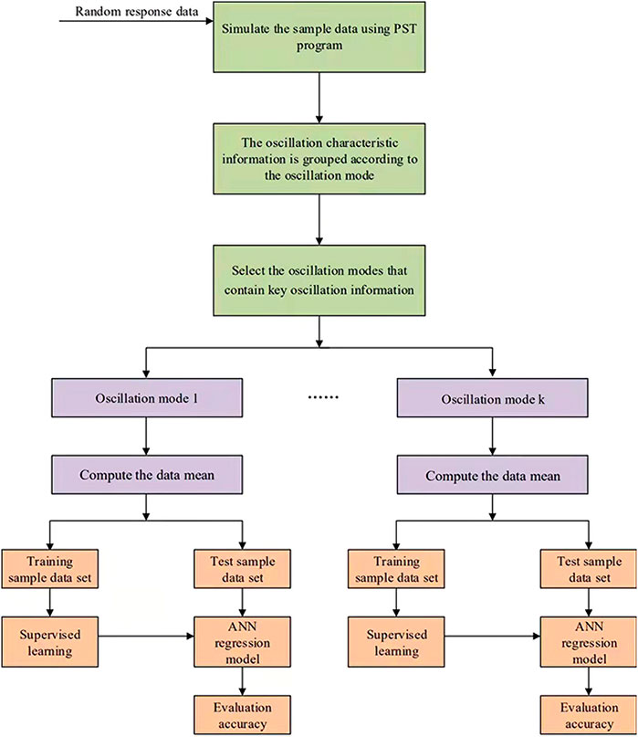
FIGURE 2. Electromechanical oscillation mode parameter identification model based on the R-M-ANN.

As the multilayer artificial neural network model requires a large number of data, and the random response data of the timing sequence are too small to support the R-M-ANN training; hence, a large number of data samples are needed. Therefore, the sliding window method is adopted to select the sample set of window data 2,000 times as the input of the artificial neural network model.

The key characteristic information in this paper selects relevant information of frequency and damping ratio. According to the magnitude of the oscillation frequency, the oscillation mode can be divided into local oscillation and interregional oscillation. The local oscillation frequency is relatively high, generally 0.7–2 Hz, while the inter-area oscillation frequency is 0.1–0.7 Hz. Interarea low-frequency oscillation makes a more serious oscillation mode because it involves the dynamic process of a large number of generators in the system.

The loss function of the model is selected as the mean square error function; when the sample size is fixed, the index used to evaluate the quality of a point estimate is always the function of the distance between the point estimate and the true value of the parameter. The most commonly used function is the square of the distance. Due to the randomness of the estimator, the expectation can be obtained from this function, which is expressed as

$MSE\left(\widehat{\theta }\right)=E{\left(\widehat{\theta }-\theta \right)}^2(28)$

When the data set is input into the trained neural network, the average error of the key feature information result E is

$E=\sqrt{\frac{1}{H}{\displaystyle \sum }_{i=1}^M{\left(\frac{\left|z_i^{\prime }-z_i\right|}{\left|z_i\right|}\right)}^2}(29)$

where H is the number of test data sets, z_i′ is the calculation results of the characteristic parameters of oscillation of this method, and z_i is the calculation result of the characteristic parameters of oscillation of the randomized-DMD method.

With a large-scale interconnected power system, a power grid operation mode, a diversified structure, all kinds of new electric components of access, and construction of the smart grid, the power system is faced with a high dynamic model dimension when the volatility is high, and the effective use of small disturbance stability is the precondition of power system stability. The WAMS can collect system data in real-time, data-driven methods can quickly analyze the stable state of the system, and the combination of the two can achieve fast online analysis. Based on the above-mentioned starting point, this paper mainly has the following innovations:

1. Input variables only depend on the measured data

Randomized dynamic mode decomposition (randomized-DMD) can identify the electromechanical oscillation mode parameters. However, the randomized-DMD needs to accumulate a certain number of data for identification, and a large number of new energy sources such as wind power and photovoltaics are connected to the power system, which poses certain challenges to the real-time identification of mechanical and electrical oscillation parameters.

Most methods of numerical calculation require parameters of each element in the power system, but the component parameters are difficult to obtain sometimes in the actual system; the method only using the WAMS can monitor variables (generator speed, power angle, and active power); the data acquisition in the system is convenient, and the input data can be collected by real-time update for steady-state tracking assessment.

2. Rapid evaluation speed

As a data-driven approach is adopted to evaluate the stability of small disturbances, there is no need to build a complex dynamic model inside the power system. When the R-M-ANN model is well-trained, only one forward calculation process is needed to calculate the electromechanical oscillation parameter of the system. Since the forward calculation process is composed of simple basic operations, the calculation complexity is low, and the calculation time is fast. In addition, since the input variables can be obtained by the WAMS in real-time, the real-time performance of the small disturbance stability assessment is further improved.

4 Case Study

4.1 Calculation and Analysis of 4-Generator 2-Area System

This section takes the 4-generator 2-area system as an example and uses the randomized DMD algorithm to quickly identify the mode parameters of the power system for simulation analysis. The results of frequency and damping ratio of electromechanical oscillation modes are obtained as the target data set of R-M-ANN model training. The structure of the 4-generator 2-area system is shown in Figure 3.

FIGURE 3

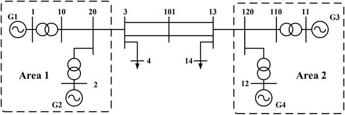
FIGURE 3. Single-line diagram for the 4-generator 2-area power system.

The sliding window sample contains the generator speed, power angle, and active power with 3% random load fluctuation. We choose 2,000 sliding windows, and each sliding window uses the randomized-DMD algorithm to calculate the sliding window sample. Table 1 shows the identification results of the randomized-DMD algorithm and small-signal stability analysis (SSSA).

TABLE 1

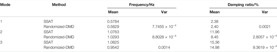
TABLE 1. Randomized-DMD electromechanical oscillation mode parameter identification results for the four-generator two-area system.

During the training process, the R-M-ANN model with the damping ratio is selected as an example to demonstrate the regression effect, as well as the error distribution diagram of the R-M-ANN model with the damping ratio of three oscillation modes, which are shown in Figure 4 and Figure 5.

FIGURE 4

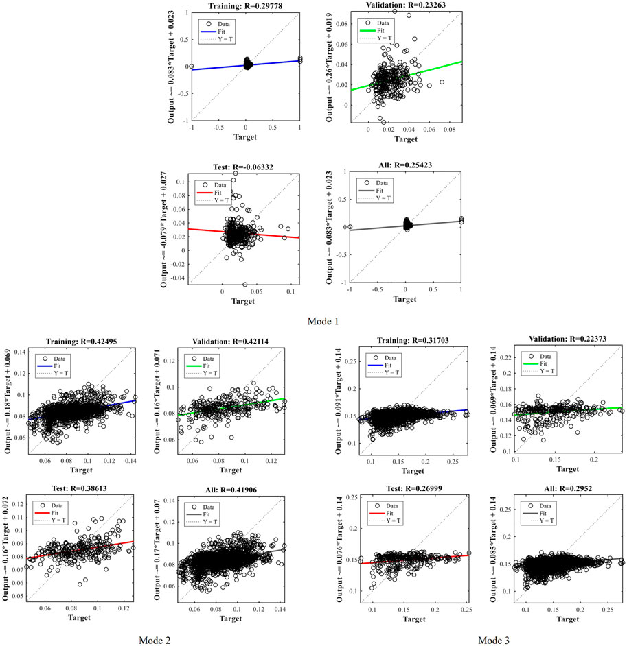
FIGURE 4. R-M-ANN model training regression chart for mode 3.

FIGURE 5

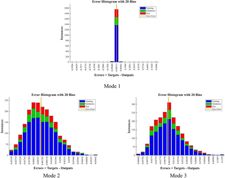
FIGURE 5. Error histogram of R-M-ANN model training.

Taking the regression diagram of mode 1 as an example, the R-M-ANN model in the weakly damped mode has a particularly good regression effect, and the point density of the training and test data sets is high, which is shown in Figure 4.

The error distribution diagram in Figure 5 shows the error distribution of data training, which can be obtained from the error distribution of the three graphs. The data error quantity decreases from zero error to a larger error distribution in turn and is uniformly distributed around the zero-error line.

Thus, it can be seen that R-M-ANN regression has a very good effect, with small data fluctuations and a small proportion of data with large errors.

It can be concluded from Table 2 that different random response data can be obtained by calculating the change in ambient excitation, and the applicability and accuracy of the R-M-ANN model can be further verified through different random response data. It can be found from the results that changing the ambient excitation has little effect on the results, the mean error of the frequency and damping ratio of all the models is very small, and the variance is also very small. For example, mode 1 is weakly damped, and the R-M-ANN model can accurately identify the weakly damped mode. Under 7% ambient excitation, the mean damping ratio of the interregional oscillation of the system is 2.42%, and the variance is 0.0030.

TABLE 2

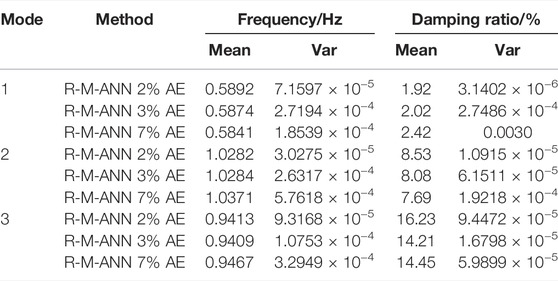
TABLE 2. Identification results for the R-M-ANN model with different ambient excitations (AEs) for the four-generator two-area system.

As can be seen from Table 3, for the same sample, the training time of the R-M-ANN is one order of magnitude smaller than that of the other two machine learning methods, which can achieve a relatively fast update and retraining of the training set, and the R-M-ANN’s performance on the test set is also significantly better than that of the other two methods. There are two main reasons for this difference. On the one hand, with the increase in the system scale, shallow learning methods will have the problem of dimension disaster, resulting in long optimization time. However, the R-M-ANN can adjust its structure flexibly, and its weight sharing attribute forces the network to train fewer parameters to achieve faster training. On the other hand, the shallow learning method has a weak learning ability for high-dimensional data and cannot extract its features from a large amount of input information, resulting in a weak generalization ability.

TABLE 3

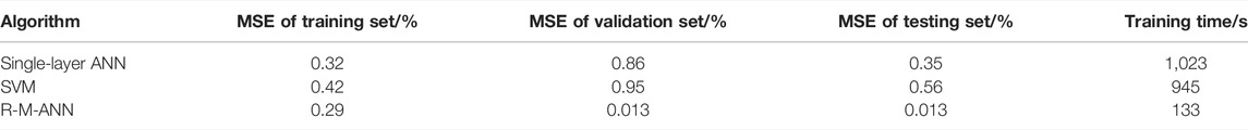
TABLE 3. Comparison of three machine-learning techniques for the 4-generator 2-area system.

4.2 Calculation and Analysis of 16-Generator 5-Area System

The 16-generator 5-area system includes 16 generators, 68 nodes, and 83 lines, which is shown in Figure 6.

FIGURE 6

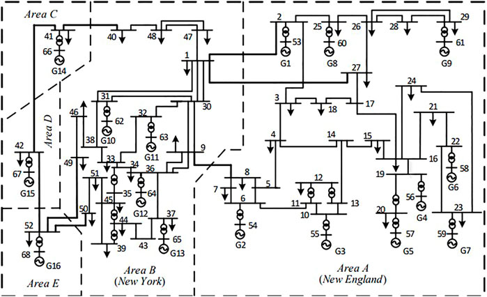
FIGURE 6. Single-line diagram for the 16-generator 5-area power system.

Depending on the size of the system input, the R-M-ANN structure is designed as follows: The first layer is the input layer, there are ten hidden layers in the middle, and the last layer is the output layer. To verify the accuracy and effectiveness of the R-M-ANN method proposed for the identification of modal parameters of the power system and to simulate the random fluctuation of the actual system load, this paper assumes that the load at node 4 and node 14 fluctuates randomly at 5% of the basic operating value. The random response data selected for R-M-ANN model training include generator speed, power angle, and active power.

Using the randomized-DMD algorithm for calculation, random response data are selected with a duration of 5,000 s as the basis, taking 50 s as the data window, and the calculation window data are slid every 2 s, sliding 2,000 times; the average value of the statistical results is shown in Table 4.

TABLE 4

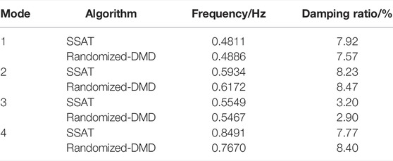
TABLE 4. Randomized-DMD electromechanical oscillation mode parameter identification results for the 16-generator 5-area system.

For these four inter-area oscillation modes, the statistical means of each sliding window data are selected as the input of the R-M-ANN, and the statistical means of frequency and damping ratio are selected as the training target; 70% of the sample data are used as the training set, 15% of the sample data are used as the validation set, and 15% of the sample data are used as the test set.

After training the R-M-ANN model, we need to test the feasibility and accuracy of the model. Therefore, assuming that the load at node 4 and node 14 fluctuates randomly at 3% of the basic operating value, we choose the same random response data with a duration of 5,000 s as the basis, taking 50 s as the data window, and slide the calculation window data every 2 s, sliding 2,000 times; the mean value of the statistical results is selected as the measured data set using the R-M-ANN model and the randomized-DMD algorithm to calculate the measured data set. The comparison of the results of frequency and damping ratio for four main inter-area oscillation modes is carried out.

From Table 5, four interval oscillation mode frequencies and damping ratios can be recognized by the two methods. Using mode 3 (weakly damped mode) as an example for two algorithms, two kinds of pattern recognition for the damping ratio are obtained as 2.90% and 3.32%, respectively. It can be seen that the mean value of the two methods is similar to the statistical average results, but the R-M-ANN model identification results have a small variance; hence, it is proved that the R-M-ANN model has stronger stability.

TABLE 5

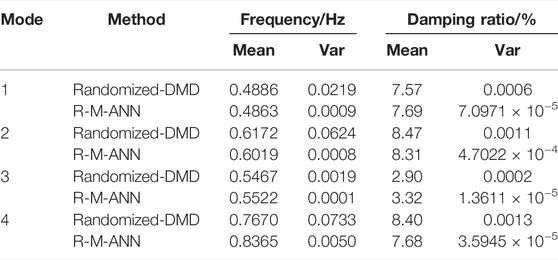
TABLE 5. Identification results for the R-M-ANN model with different ambient excitations for the 16-generator 5-area system.

As can be seen from the frequency histogram (Figure 7), every kind of inter-area oscillation mode is evenly distributed near the average value as a uniform measure of reduction; it proves that the R-M-ANN model recognition has good stability, the calculation results are more accurate from the frequency histogram for four inter-area oscillation mode damping ratios.

FIGURE 7

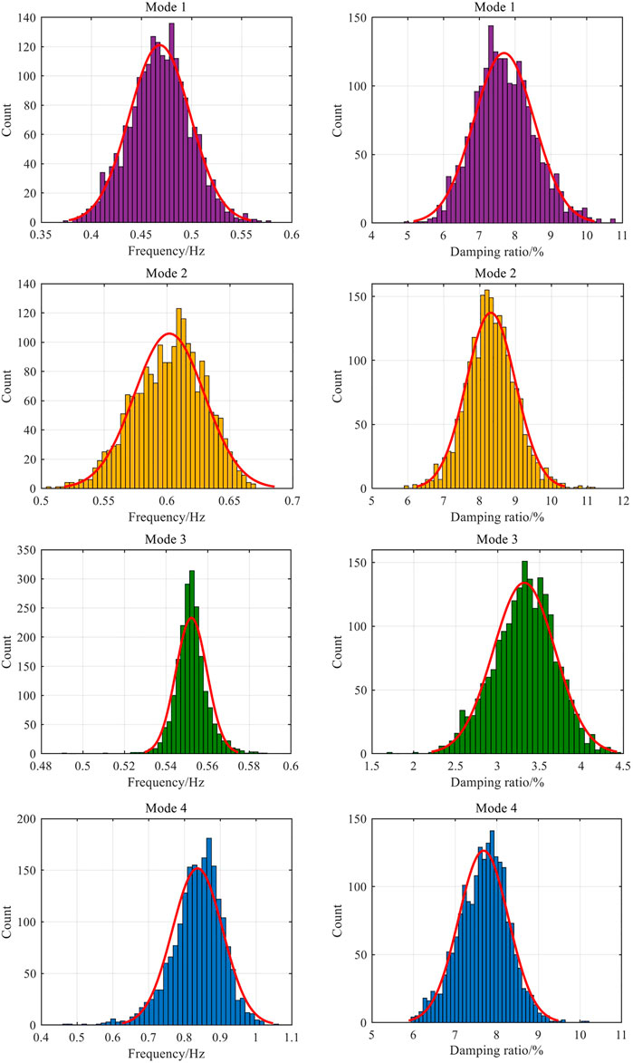
FIGURE 7. Frequency histogram of frequency and damping ratio of four interval oscillation modes for the 16-generator 5-area system.

In the electromechanical oscillation parameter identification process, the operation mode of a small-scale change seriously affects the system safety and stable operation, and the operation mode changes directly affect the damping of the system level. Therefore, it is important to verify the R-M-ANN model under the condition of operation mutation of damping level tracking precision. Due to the continuous increase in grid-connected scale and the capacity of new energy, the operation mode of the modern power grid is very complex, and small-scale operation mode changes often occur, which seriously affects the safe and stable operation of the system. In the stability assessment of electromechanical small disturbances, the change in operation mode directly affects the damping level of the system. To verify the multilayer artificial neural network under the condition of the operation mode mutation of damping level tracking precision, the R-M-ANN studies the data offline with a large number of running modes.

Using mode 3 as an example, suppose that the power system operation mode has changed the system at 20 and 25 s, randomized-DMD calculation results show that the damping ratio increased from 2.9% to 9.2% at 20 s and then increase to 12.4% at 25 s. The online tracking result of the damping ratio of the R-M-ANN model is shown in Figure 8.

FIGURE 8

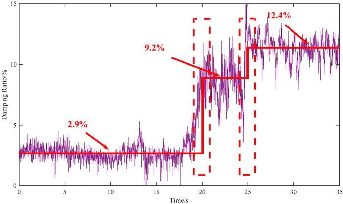
FIGURE 8. Identification results of the interval oscillation damping ratio under the abrupt operation mode.

From Figure 8, we can see that the R-M-ANN model can accurately track the change in the damping ratio. The curve changes at 20 and 25 s. The curve is stable before and after the change and fluctuates slightly around the mean value.

At the same time, since the computing time of the R-M-ANN model can be ignored, if the system operation mode changes, the damping ratio of the system changes, and the R-M-ANN model can accurately track this situation without time delay, providing a certain time margin for the scheduler to make a damping modulation strategy.

5 Conclusion

For deep learning methods, accuracy is essential, and generalization ability is more important. In this paper, an R-M-ANN-based electromechanical oscillation mode parameter identification method is proposed, which can calculate the key characteristic information of the power system in real-time by monitoring the data of the WAMS and verify the reliability of the 4-generator 2-area system and the IEEE 16-generator 5-area system. The conclusions are shown as follows:

• The R-M-ANN model for the random response of the input data is an effective identification method for the local oscillation mode and inter-area oscillation mode frequency and damping ratio and has certain adaptability to the simple network topology change; the weakly damped oscillation modes can be quickly identified without a time-delay and a power system model due to its advantages such as instantaneity; the small signals of the power system can be accurately and completely evaluated in quasi-real-time.

• Through the simulation of the 4-generator 2-area system, it can be seen that by changing the ambient excitation of motivation to three groups of random response data, the R-M-ANN model is trained for parameter identification of electromechanical oscillation mode and obtaining the result of the mean value of the frequency and damping ratio close to the results of variance, which is very small, which shows that the R-M-ANN identification method is stable and has strong robustness. The R-M-ANN can also adapt to incomplete data or abnormal data. In addition, the R-M-ANN model is more reliable than other shallow machine learning algorithms. With respect to the online tracking ability, the R-M-ANN has a sensitive tracking capability to provide real-time information to dispatchers of the power system.

In the future, the R-M-ANN needs to constantly update the likely scenario. The model can be richer, as well as the actual application. Online learning should be strengthened and combined with artificial intelligence to improve the learning efficiency.

Data Availability Statement

The raw data supporting the conclusion of this article will be made available by the authors, without undue reservation.

Author Contributions

GC carried out the concepts and design. SG carried out literature search, data acquisition, data analysis, case studies, and manuscript preparation and editing. CL performed manuscript review. All authors have read and approved the content of the manuscript and have made substantial contributions to the final approved version to be submitted.

Funding

This work was supported in part by the National Key R&D Program of China, 2021YFB2400800.

Conflict of Interest

The authors declare that the research was conducted in the absence of any commercial or financial relationships that could be construed as a potential conflict of interest.

Publisher’s Note

All claims expressed in this article are solely those of the authors and do not necessarily represent those of their affiliated organizations, or those of the publisher, the editors, and the reviewers. Any product that may be evaluated in this article, or claim that may be made by its manufacturer, is not guaranteed or endorsed by the publisher.

References

Anderson, M. G., Zhou, N., Pierre, J. W., and Wies, R. W. (2005). Bootstrap-Based Confidence Interval Estimates for Electromechanical Modes from Multiple Output Analysis of Measured Ambient Data. IEEE Trans. Power Syst. 20 (2), 943–950. doi:10.1109/TPWRS.2005.846125

CrossRef Full Text | Google Scholar

Angelidis, G., and Semlyen, A. (1996). Improved Methodologies for the Calculation of Critical Eigenvalues in Small Signal Stability Analysis. IEEE Trans. Power Syst. 11 (3), 1209–1217. doi:10.1109/59.535592

CrossRef Full Text | Google Scholar

Chan, S., and Nopphawan, P. (2020). “Artificial Intelligence-Based Approach for Forced Oscillation Source Detection and Classification,” in 2020 8th International Conference on Condition Monitoring and Diagnosis (CMD), Phuket, Thailand, October 25–28, 186–189. doi:10.1109/CMD48350.2020.9287262

CrossRef Full Text | Google Scholar

De La Ree, J., Centeno, V., Thorp, J. S., and Phadke, A. G. (2010). Synchronized Phasor Measurement Applications in Power Systems. IEEE Trans. Smart Grid 1 (1), 20–27. doi:10.1109/TSG.2010.2044815

CrossRef Full Text | Google Scholar

Dosiek, L., Pierre, J. W., and Follum, J. (2013). A Recursive Maximum Likelihood Estimator for the Online Estimation of Electromechanical Modes with Error Bounds. IEEE Trans. Power Syst. 28 (1), 441–451. doi:10.1109/TPWRS.2012.2203323

CrossRef Full Text | Google Scholar

Drineas, P., and Mahoney, M. W. (2016). RandNLA: Randomized Numerical Linear Algebra. Commun. ACM 59 (6), 80–90. doi:10.1145/2842602

CrossRef Full Text | Google Scholar

Gershenson, C. (2003). Artificial Neural Networks for Beginners. arXiv preprint cs/0308031.

Google Scholar

Goh, A. T. C. (1995). Back-Propagation Neural Networks for Modeling Complex Systems. Artif. Intell. Eng. 9 (3), 143–151. doi:10.1016/0954-1810(94)00011-S

CrossRef Full Text | Google Scholar

Kenji, S. (2011). Artificial Neural Networks: Methodological Advances and Biomedical Applications. Rijeka, Croatia: BoD–Books on Demand.

Google Scholar

Khalilinia, H., and Venkatasubramanian, V. (2017). Recursive Frequency Domain Decomposition for Multidimensional Ambient Modal Estimation. IEEE Trans. Power Syst. 32 (1), 822–823. doi:10.1109/TPWRS.2016.2558466

CrossRef Full Text | Google Scholar

Khalilinia, H., Zhang, L., and Venkatasubramanian, V. (2015). Fast Frequency-Domain Decomposition for Ambient Oscillation Monitoring. IEEE Trans. Power Deliv. 30 (3), 1631–1633. doi:10.1109/TPWRD.2015.2394403

CrossRef Full Text | Google Scholar

Li, Y., Geng, G., and Jiang, Q. (2016). An Efficient Parallel Krylov-Schur Method for Eigen-Analysis of Large-Scale Power Systems. IEEE Trans. Power Syst. 31 (2), 920–930. doi:10.1109/TPWRS.2015.2418272

CrossRef Full Text | Google Scholar

Lima, D., and Alden, (1994). “Neural Network Assessment of Small Signal Stability,” in 1994 Proceedings of Canadian Conference on Electrical and Computer Engineering, Halifax, CA, September 25–28, 2, 730–733. doi:10.1109/CCECE.1994.405855

CrossRef Full Text | Google Scholar

Liu, J., Yang, Z., Zhao, J., Yu, J., Tan, B., and Wenyuan, L. (2021). Explicit Data-Driven Small-Signal Stability Constrained Optimal Power Flow. IEEE Trans. Power Syst., 1–1. doi:10.1109/TPWRS.2021.3135657

CrossRef Full Text | Google Scholar

Ma, J., Dong, Z. Y., and Zhang, P. (2006). Comparison of BR and QR Eigenvalue Algorithms for Power System Small Signal Stability Analysis. IEEE Trans. Power Syst. 21 (4), 1848–1855. doi:10.1109/TPWRS.2006.883685

CrossRef Full Text | Google Scholar

Mohammadi, M., and Gharehpetian, G. B. (2009). Application of Multi-Class Support Vector Machines for Power System On-Line Static Security Assessment Using DT - Based Feature and Data Selection Algorithms. J. Intelligent Fuzzy Syst. 20, 133–146. doi:10.3233/ifs-2009-0421

CrossRef Full Text | Google Scholar

Mohammadi, M., Gharehpetian, G. B., and Niknam, T. (2010). On-Line Small-Signal Stability Assessment of Power Systems Using Ball Vector Machines. Electr. Power Components Syst. 38 (13), 1427–1445. doi:10.1080/15325001003735150

CrossRef Full Text | Google Scholar

Mohammadi, M., and Gharehpetian, G. B. (2008). Power System On-Line Static Security Assessment by Using Multi-Class Support Vector Machines. J. Appl. Sci. 8 (12), 2226–2233. doi:10.3923/jas.2008.2226.2233

CrossRef Full Text | Google Scholar

Nezam Sarmadi, S. A., and Venkatasubramanian, V. (2014). Electromechanical Mode Estimation Using Recursive Adaptive Stochastic Subspace Identification. IEEE Trans. Power Syst. 29 (1), 349–358. doi:10.1109/TPWRS.2013.2281004

CrossRef Full Text | Google Scholar

Phadke, A. G. (2002). “Synchronized Phasor Measurements-A Historical Overview,” in IEEE/PES Transmission and Distribution Conference and Exhibition, Yokohama, Japan, October 6–10, 1, 476–479. doi:10.1109/TDC.2002.1178427

CrossRef Full Text | Google Scholar

Pierre, J. W., Trudnowski, D. J., and Donnelly, M. K. (1997). Initial Results in Electromechanical Mode Identification from Ambient Data. IEEE Trans. Power Syst. 12 (3), 1245–1251. doi:10.1109/59.630467

CrossRef Full Text | Google Scholar

Rai, A. K., Kaushika, N. D., Singh, B., and Agarwal, N. (2011). Simulation Model of ANN Based Maximum Power Point Tracking Controller for Solar PV System. Sol. Energy Mater. Sol. Cells 95 (2), 773–778. doi:10.1016/j.solmat.2010.10.022

CrossRef Full Text | Google Scholar

Ravikumar, G., and Govindarasu, M. (2020). Anomaly Detection and Mitigation for Wide-Area Damping Control Using Machine Learning. IEEE Trans. Smart Grid, 1–1. doi:10.1109/TSG.2020.2995313

CrossRef Full Text | Google Scholar

Shair, J., Li, H., Hu, J., and Xie, X. (2021). Power System Stability Issues, Classifications and Research Prospects in the Context of High-Penetration of Renewables and Power Electronics. Renew. Sustain. Energy Rev. 145, 111111. doi:10.1016/j.rser.2021.111111

CrossRef Full Text | Google Scholar

Shi, L., Gu, W., Fan, C., Dou, R., Yi, W., and Yu, Y. (2020). “Identification of Low Frequency Oscillation Mechanism Based on Deep Learning,” in 2020 12th IEEE PES Asia-Pacific Power and Energy Engineering Conference (APPEEC), Nanjing, China, September 20–23, 1–6. doi:10.1109/APPEEC48164.2020.9220585

CrossRef Full Text | Google Scholar

Teeuwsen, S. P., Erlich, I., and El-Sharkawi, M. A. (2003). “Neural Network Based Classification Method for Small-Signal Stability Assessment,” in 2003 IEEE Bologna Power Tech Conference Proceedings, Bologna, Italy, June 23–26, 3, 6. doi:10.1109/PTC.2003.1304415

CrossRef Full Text | Google Scholar

Teoh, E. J., Tan, K. C., and Xiang, C. (2006). Estimating the Number of Hidden Neurons in a Feedforward Network Using the Singular Value Decomposition. IEEE Trans. Neural Netw. 17 (6), 1623–1629. doi:10.1109/TNN.2006.880582

PubMed Abstract | CrossRef Full Text | Google Scholar

Tu, J. H., Rowley, C. W., Luchtenburg, D. M., Brunton, S. L., and Kutz, J. N. (2014). On Dynamic Mode Decomposition: Theory and Applications. J. Comput. Dyn. 1 (2), 391–421. doi:10.3934/jcd.2014.1.391

CrossRef Full Text | Google Scholar

Wies, R. W. (1999). Estimating Low-Frequency Electromechanical Modes of Power System Using Ambient Data. Ph.D. dissertation. Laramie, Wyoming: University of Wyoming.

Google Scholar

Wies, R. W., Pierre, J. W., and Trudnowski, D. J. (2003). “Use of ARMA Block Processing for Estimating Stationary Low-Frequency Electromechanical Modes of Power Systems,” in 2003 IEEE Power Engineering Society General Meeting (IEEE Cat. No.03CH37491), Toronto, CA, July 13–17, 2096. doi:10.1109/PES.2003.1270937

CrossRef Full Text | Google Scholar

You, S., Zhao, Y., Mandich, M., Cui, Y., Li, H., Xiao, H., et al. (2020). “A Review on Artificial Intelligence for Grid Stability Assessment,” in 2020 IEEE International Conference on Communications, Control, and Computing Technologies for Smart Grids, 1–6. doi:10.1109/SmartGridComm47815.2020.9302990

CrossRef Full Text | Google Scholar

Zhou, N., Pierre, J. W., Trudnowski, D. J., and Guttromson, R. T. (2007). Robust RLS Methods for Online Estimation of Power System Electromechanical Modes. IEEE Trans. Power Syst. 22 (3), 1240–1249. doi:10.1109/TPWRS.2007.901104

CrossRef Full Text | Google Scholar

Zhou, N., Trudnowski, D. J., Pierre, J. W., and Mittelstadt, W. A. (2008). Electromechanical Mode Online Estimation Using Regularized Robust RLS Methods. IEEE Trans. Power Syst. 23 (4), 1670–1680. doi:10.1109/TPWRS.2008.2002173

CrossRef Full Text | Google Scholar

Zupan, J. (1994). Introduction to Artificial Neural Network (ANN) Method: What They Are and How to Use Them. Acta Chim. Slov. 41 (3), 327–352.

Google Scholar