A Short-Term Wind Power Forecast Method via XGBoost Hyper-Parameters Optimization

The improvement of wind power prediction accuracy is beneficial to the effective utilization of wind energy. An improved XGBoost algorithm via Bayesian hyperparameter optimization (BH-XGBoost method) was proposed in this article, which is employed to forecast the short-term wind power for wind farms. Compared to the XGBoost, SVM, KELM, and LSTM, the results indicate that BH-XGBoost outperforms other methods in all the cases. The BH-XGBoost method could yield a more minor estimated error than the other methods, especially in the cases of wind ramp events caused by extreme weather conditions and low wind speed range. The comparison results led to the recommendation that the BH-XGBoost method is an effective method to forecast the short-term wind power for wind farms.

1 Introduction

In recent years, as the pace of global carbon reduction has accelerated, China’s “carbon neutrality” task has clarified the direction of China’s energy transition. It is imperative to develop clean and sustainable renewable energy. As an efficient, non-polluting, zero-emission renewable energy source, wind energy has become an important measure to solve the energy crisis. However, wind’s intermittent and random nature causes uncertainty and instability in wind power generation, which leads to difficulties in dispatching and low efficiency in grid connection (Quan et al., 2019; Santhosh et al., 2020; Maldonado-Correa et al., 2021). Accurate wind power forecast is beneficial to optimize the operation and dispatch of power systems, develop reasonable control strategies, improve energy storage efficiency and maximize economic benefits (Zhang et al., 2021, 2017). Therefore, timely and accurate wind forecasts are essential for the safe operation of the grid and the planning of electricity market transactions (Wang et al., 2017; Han et al., 2018).

For time scale, wind power forecast includes ultra-short-term, short-term, medium-term and long-term power forecast (Tian, 2021). Ultra-short-term forecast is used to predict power generation in the next few hours based on historical data, which is helpful for controlling the daily operation of wind farm units. Short-term forecast is used to predict in advance for several hours to several days, which is helpful for the rationality of the economic system and maintenance of the wind turbine. The medium-long term forecast is used to predict in advance for several days to several months,which is helpful for making quarterly power generation plans for grid and wind farm construction (Ju et al., 2019; Li L. et al., 2020).

Due to the uncertainty of the wind power system, the time scale of the current wind power prediction results mostly focuses on the short-term forecast (Tian, 2021). The physical, statistical, artificial intelligence and ensemble methods are usually used to forecast short-term wind power (Hanifi et al., 2020). The physical model uses micro-scale meteorology and fluid mechanics to convert the numerical weather forecast (NWP) data into wind speed, and wind direction data at the height of the wind turbine and finally matches the wind turbine power curve. The prediction accuracy of the physical model mainly depends on the accuracy of the numerical weather forecast (NWP) data and the accuracy of the geographical environment around the wind farm (Rodríguez et al., 2020). The statistical method is based on historical wind power data through curve fitting and parameterization methods to predict wind power. Hao (2019) designed an extreme learning machine prediction method based on variational mode decomposition feature extraction. The ELM model is optimized with a multi-objective gray wolf optimizer using historical wind power time series data as input. Finally, a high-precision wind power prediction time series hybrid model is obtained. Zameer et al. (2015) proposed a new short-term wind power prediction method based on the machine learning method (STWP). This method combines machine learning technology with feature selection and regression. The proposed method is a hybrid maximum likelihood model, which uses feature selection through irrelevant and redundant filters, and then uses a support vector regression machine for auxiliary prediction, And finally realizes wind power forecasting. Sideratos and Hatziargyriou (2020) proposed an improved radial basis function neural network for wind power prediction. The method has better results than others, but the iterative convergence process is longer. Liu et al. (2018) proposed a short-term wind speed and wind prediction model based on singular spectrum analysis and Locality-sensitive Hashing (LSH). To deal with the high volatility of the original time series, SSA is used to decompose it into two components. The two components are reconstructed in the phase space to obtain the average trend and fluctuation components. Then, LSH is used to select similar segments of the intermediate trend segment for local prediction, thereby improving the accuracy and efficiency of prediction.

The above methods, mainly from the perspective of clustering, combination, deep neural network, and other considerations, improve wind power prediction accuracy. The choice of hyperparameters in the algorithm is also crucial. The same algorithm with different datasets and different hyperparameters can have additional prediction precision. Therefore, this article proposed a new short-term wind power forecast mehtod named BH-XGBoost, which sets up Hyper-parameter optimization during the model training process to optimize and improve the performance of XGBoost (Yang et al., 2019; Zheng and Wu, 2019). Finally, BH-XGBoost is verified through wind farm turbine data and numerical weather forecast data.

The remainder of this article is arranged as follows. Section 2 introduced the dataset used in this study. Section 3 described the method of BH-XGBoost. Results and discussion in Section 4 and conclusion in Section 5.

2 Data

2.1 Wind Farm Data

In order to verify the effectiveness of the proposed method, the real data of a wind farm is employed to test the BH-XGBoost method. The target wind farm locates on the east coast of Jiangsu province in China (as shown in Figure 1). The wind farm data includes the historical wind power of each wind farm and wind speed from SCADA system of the wind turbines, and all the data were subjected to strict quality control. The target wind farm has 100 wind turbines with 2 MW rated power, and the hub height of the wind turbine is 100 m. The frequency of the power and wind data collection is 15 min from October 2020 to December 2021.

FIGURE 1

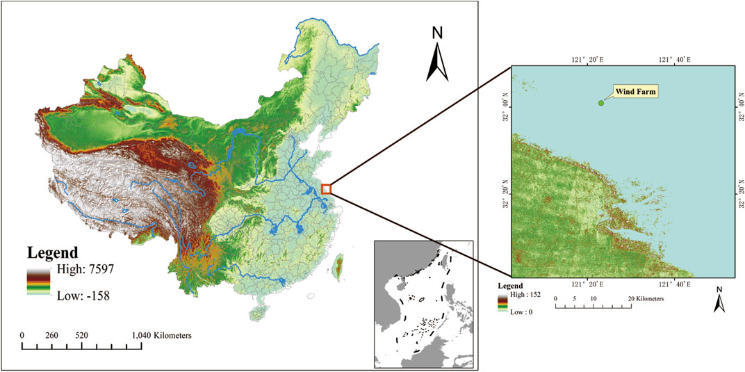
FIGURE 1. The location of the target wind farm.

2.2 Numerical Weather Forecast Data

In this study, Numerical weather forecasting (NWP) is employed to provide weather data for the next 1–3 days. NWP is based on the actual conditions of the atmosphere. Given initial conditions and boundary conditions, numerical calculations are carried out by large-scale computers, and atmospheric motion equations are solved numerically. The atmospheric state at the initial time is known to predict the initial state of the future moment. The numerical weather prediction system is based on Weather Research and Forecast (WRF), a mesoscale weather model. It mainly realizes a small area weather forecast with a resolution of fewer than 10 km and a time scale of 3 days. The WRF model has advanced data assimilation technology, powerful nesting capabilities, and advanced physical processes. High-quality NWP data can improve the forecast accuracy of the short-term wind power prediction greatly. The NWP data of the target wind farm is from the China Meteorological Administration (CMA), which is updated twice a day with a temporal resolution of 15 min, the spatial resolution is 1.0 km × 1.0 km, and for a predicted length of 144 h. The output of the NWP elements includes wind speed (m/s), temperature (°C), relative humidity (%), and pressure (hPa). Figure 2 is the basic flow chart of the WRF model for this research.

FIGURE 2

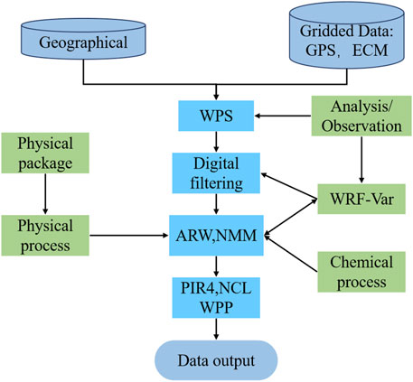
FIGURE 2. The flow chart of WRF model.

3 Methods

3.1 XGBoost Algorithm

The XGBoost algorithm (eXtreme Gradient Boosting) is optimized and improved based on the gradient progressive regression tree algorithm. Once it appeared, it has received widespread attention for its excellent learning effect and efficient training model speed (Kumar et al., 2020; Phan et al., 2020). The algorithm can effectively construct a boosting tree and perform parallel operations while effectively using the multi-threading of the CPU. This algorithm has achieved excellent results in Kaggle’s Higgs sub-signal recognition competition and has been widely concerned. Its core is to pre-order all features and enhances classification trees and decision trees. XGBoost is an integrated model consisting of k decision trees, the predicted value is calculated from:

${\widehat{y}}_i=\sum _{t=1}^k{f}_t\left(x_i\right),(1)$

${\widehat{y}}_i$ is the predicted value of x_i. f_t represents a decision tree, and f_t (x_i) is the predicted value of f_t given x_i. Then the loss function L can be expressed in terms of predicted value ${\widehat{y}}_i$ and true values y_i:

$L=\sum _{i=1}^{n}l\left(y_i,{\widehat{y}}_i\right).(2)$

To avoid overfitting and improve the model’s generalization ability, the regular term Ω is usually added to the equation. The loss function can be rewritten as Eq. 3, and the regular term Ω(f_t) define as Eq. 4, where T denotes the number of leaf nodes and w_jrefers to the weight of the jth leaf node.

$Obj=\sum _{i=1}^{n}l\left({\widehat{y}}_i,y_i\right)+\sum _{t=1}^k\mathrm{\Omega }\left(f_t\right),(3)$

$\mathrm{\Omega }\left(f_t\right)=\gamma T+\frac{1}{2}\lambda \sum _{j=1}^T{w}_j^2.(4)$

XGBoost uses a forward addition strategy where each time the model adds a decision tree, it learns a new function and its coefficients to fit the residuals of the last step of the prediction. Therefore, using the model at step t as an example, the prediction for the ith sample x_i is as Eq. 5 and the object function of step t is as Eq. 6.

${\widehat{y}}_i^t={\widehat{y}}_i^{t-1}+f_t\left(x_i\right),(5)$

${\mathrm{Obj}}^{\left(t\right)}=\sum _{i=1}^{n}L\left(y_i,{\widehat{y}}^{t-1}+f_t\left(x_i\right)\right)+\mathrm{\Omega }\left(f_t\right).(6)$

Use Taylor expansion to expand the above equation:

${\mathrm{Obj}}^{\left(t\right)}\approx \sum _{i=1}^n\left[L\left(y_{i,}{\widehat{y}}^{t-1}\right)+g_i{f}_t\left(x_i\right)+\frac{1}{2}{h}_i{f}_t^2\left(x_i\right)\right]+\mathrm{\Omega }\left(f_t\right).(7)$

Among them, g_i represents the first derivative of $L(y_i,{\widehat{y}}^{t-1})$ to ${\widehat{y}}^{t-1}$, and h_i represents the second derivative of $(y_i,{\widehat{y}}^{t-1})$ to ${\widehat{y}}^{t-1}$. In addition, you can merge the same function values on the same leaf node. So the final deduced result is:

$w_j=-\frac{G_j}{H_j+\lambda }.(8)$

Therefore, substituting w_j into the objective function is simplified as:

${\mathrm{Obj}}^{\left(t\right)}=-\frac{1}{2}\sum _{j=1}^T\frac{G_j^2}{H_J+\lambda }+\gamma T+C.(9)$

The above equation simplifies the objective function. It is evident that XGBoost can customize the objective function, use only the first derivative and the second derivative in the calculation process, and obtain the simplified equation. XGBoost parameter selection is significant. Table 1 shows the specific parameter types of the XGBoost algorithm (Zheng et al., 2017; Li K. et al., 2020).

The parameters max_depth and learing_rate will determine the performance of the XGBoost algorithm model.

TABLE 1

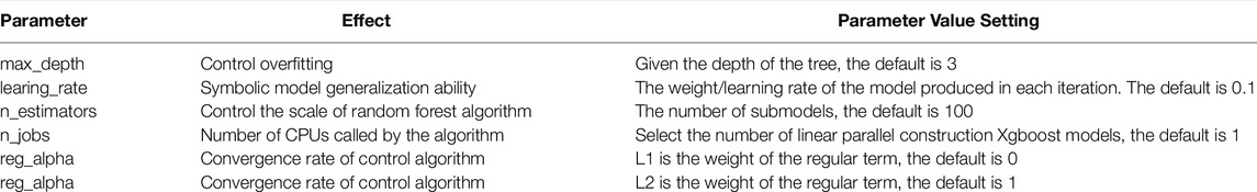
TABLE 1. XGBoost various parameters.

3.2 Hyper-Parameter Principle

Hyper-parameter is the frame parameters in the machine learning model. The hyper-parameters are the number of classes in the clustering method, the number of topics in the topic model, etc. Machine learning algorithms have been widely used in various fields. Its hyper-parameter must be adjusted to adapt the machine learning model to different problems (Zhou et al., 2017; Huang et al., 2021).

In this article, Bayesian hyper-parameter optimization is selected. The goal of network learning is to determine the mapping y = f (x, θ), y is the output, x is the input vector, and the vector determines the size of the mapping. The main idea of Bayesian optimization is adjusting the hyper-parameter of a given model to establish a probability model of the objective function. Using the acquisition function to perform an effective search before selecting the optimal hyper-parameter set and selecting the optimal hyper-parameter set (Wang et al., 2021). Taking the hyper-parameter θ in GBRT as a point in the multidimensional space for optimization, the hyper-parameter θ that minimizes the loss function value f(θ) can be found in the set A ∈ X^d, as shown in the following equation:

${\theta }^{*}=\arg \underset{\theta \in A}{\min }f\left(\theta \right).(10)$

There is no prior knowledge about the structure of UNKNOWN, it is assumed that the noise in the observation is:

$y\left(\theta \right)=f\left(\theta \right)+\epsilon ,\text{\hspace{0.17em}and\hspace{0.17em}}\epsilon \sim N\left(0,{\sigma }_{\text{\hspace{0.17em}noise\hspace{0.17em}}}^2\right).(11)$

The Bayesian framework includes two basic options. First, a prior function p (f|D) (called a hypothesis function) must be selected to represent the hypothesis of the function to be optimized. Secondly, the posterior model establishes the acquisition function to determine the next test point.

The Bayesian framework uses hypothesis function p (f|D) to build an objective function model based on the observed data sample D. Based on the current p (f|D) model, The model chooses between optimization and development (Kotthoff et al., 2019). The main distinction of the Bayesian optimization model is the difference in surrogate functions, which generally include Tree Parzen Estimator (TPE), Random Forest, and Gaussian Process (Yoo, 2019).

3.3 BH-XGBoost Method

In this study, the hyperparameters of the XGBoost are optimized via Bayesian theory for the short-term wind power forecast. Figure 3 shows the workflow of the new method (BH-XGBoost). Before training, define the search space of each hyper-parameters based on XGBoost. The init hyper-parameters values from the search space are chosen randomly for the first iteration.

FIGURE 3

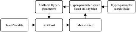
FIGURE 3. The workflow chart of BH-XGBoost.

After the first iteration, the metric results, such as MAE, MSRE, etc., will be input to the hyper-parameters algorithm. The bayesian algorithm integrates the history-measured results and searches space, and outputs each hyper-parameters value. The algorithm will kick off a new iteration while receiving the new hyper-parameters values. The algorithm will stop until the validation error is less than the threshold we set.

4 Results and Discussion

4.1 Hyper-Parameter Optimization

This article defines the four seasons based on month, Jan. for spring, Apr. for summer, Jul. for Autumn, and Oct. for Winter. The data of the first 10 days from each month are selected as the test dataset and the remaining data as the training dataset for next month. The Bayesian hyper-parameter optimization method is employed to determine the optimal XGBoost parameters. Different data sets have different selection parameters. XGBoost simplifies the model due to the addition of regularization items. At the same time, it combines the actual situation with proper pruning in the later stage, which further improves the model’s efficiency to obtain the best value. While improving the accuracy, XGBoost uses the CPU’s multi-threading to carry out parallel calculations during the application process, which significantly reduces the training time. However, the shortcoming of XGBoost is that it must traverse the entire training set in each iteration cycle. In the pre-sorting step, XGBoost retains the eigenvalues of the training dataset while retaining the evaluation results of the eigenvalues. Hyperparameter optimization searches effectively via selecting the optimal hyperparameter set and optimizing the XGBoost algorithm’s parameters as points in the multidimensional space to achieve the optimal effect of the model. In this paper, Bayesian hyper-parameter optimization is used to improve XGBoost. The input function is XGBoost hyperparameters, such as max_depth (range from 3 to 30), learing_rate (range from 0.1 to 0.15), and n_estimators (range from 100 to 1,000). The output model uses the root mean square error to solve the objective function and cross-validate. Table 2 lists the best parameters of the model for each month. The optimized parameters obtained in the default range are also different. The four data sets have no significant differences in sub-models and the maximum depth. There are differences in other model parameters. In addition, due to the various constraints between the hyperparameters, the model error will also increase as the number of adjustment parameters becomes larger. Therefore, the other model hyperparameters are randomly selected in this article.

TABLE 2

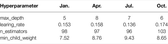
TABLE 2. XGBoost various parameters.

4.2 Sensitivity Analysis for Different Cases

In order to evaluate the new method, XGBoost, SVM, KELM, ELM, and LSTM are employed to compare the performance of BH-XGBoost. Table 3 shows the comparison results of different methods. Table 3 shows that the proposed method is more accurate than other methods. Table 3 describes the distribution of the three metrics for different methods and months. It illustrates that the root means square error (RMSE) obtained by BH-XGBoost is 21% lower than others for Jan. All the results of RMSE from other methods are around 11.7. Especially in Jul. and Oct., the proposed method is considerably better than the other methods. Also, the same results can be seen from MAE and R-square for all the cases. The results demonstrate that the proposed method is superior to the traditional machine learning methods for all the months.

TABLE 3

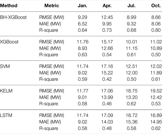
TABLE 3. The performance of different methods for three metrics.

Figure 4 compares the forecast results of the different methods for different cases. Figure 4 (a)-(d) show that the BH-XGBoost method obviously outperformance the other methods for all the cases. The forecast results curve of BH-XGBoost is the closest to the observed curve, especially in the highlighted region 1 of the callout. As the highlighted region 2 of Figure 4 (b),(d) shows, the results demonstrate that the BH-XGBoost method is superior to the other methods when the wind speed changes drastically and significantly. The BH-XGBoost method can be well adapted to both short-term wind power and ramp events caused by extreme weather conditions. Also, in the highlighted region 3 of the callout of Figure 4 (a),(c), notice that the performance of the BH-XGBoost method is better than the performance of other methods over the low wind speed. Thus, the proposed method can effectively provide wind energy utilization via the results of efficient wind power forecasting for all the cases.

FIGURE 4

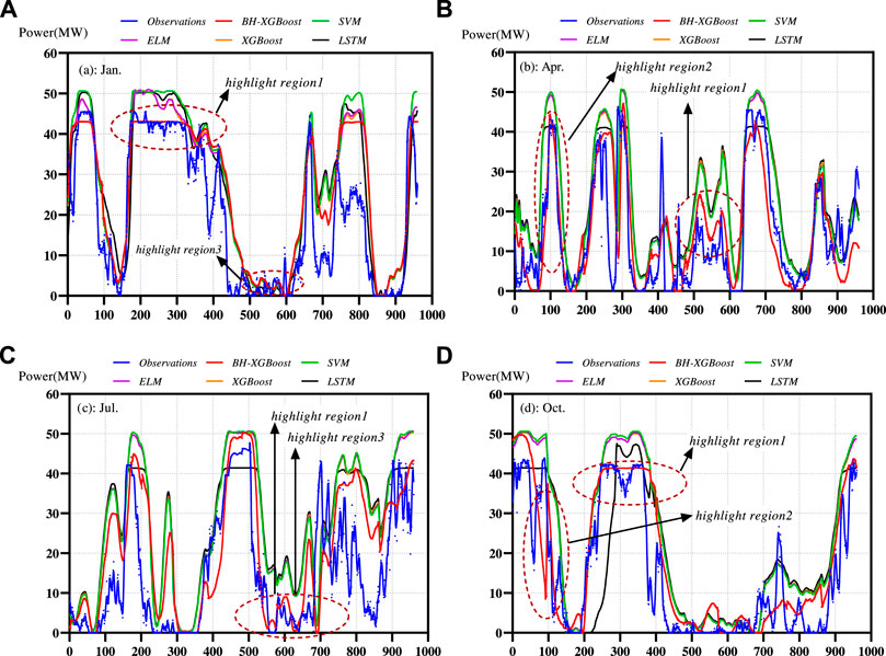
FIGURE 4. Examples of performance of the different methods for different cases: (A) Jan., (B) Apr., (C) Jul., (D) Oct.

Figure 5 illustrates the regression between observed and forecast power data for two special cases: Figure 5A for wind speed changes drastically, Figure 5B for low wind speed. Using the proposed method, the slope of the regression line has tiny gaps against the observations, which is better than the other methods (Figure 5A). Both in Figure 5A and Figure 5B, the SVM, ELM and XGBoost methods almost have the same performance. In Figure 5B, the slope of the regression for the BH-XGBoost method is not as good as the performance in Figure 5A, but considerably better than the other methods. This method is reasonable because the BH-XGBoost method has the advantages of optimal parameters, which can better simulate wind turbines’ power generation law.

FIGURE 5

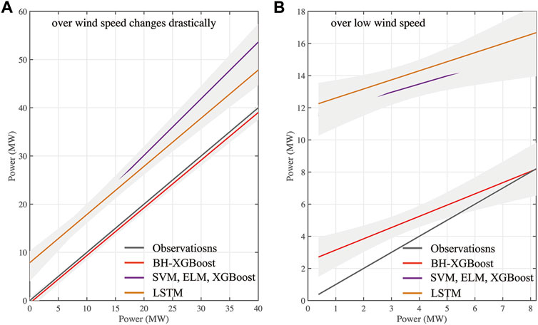
FIGURE 5. Comparison of observed to forecast power data for different methods over two special cases: (A) over wind speed changes drastically, (B) over low wind speed.

In this article, the residual boxplot is employed to analyze the center position and degree of dispersion of the residual result obtained by the different methods against the observation. Figure 6A-(d) illustrate that the residual box of BH-XGBoost outperforms others, especially in Figure 6B while the median line is infinitely close to 0. And the performance of SVM, ELM and XGBoost are similar to each other, which also can be proved to form the distribution of outliers in Figure 6D. More, the residuals of the proposed method are most concentrated among all the methods as the width of the residual box is the smallest. From Figure 6A-(d), the forecast results are generally higher than the observations. The reason is that there are power cuts and maintenance in the actual process of wind farm power generation. From the distribution of outliers, the proposed method also seems to perform better. In Figure 6A, (b), (d), the outliers that deviate from the maximum and minimum values are more homogeneous against the other methods. Noticed that all the outliers are below the minimum values in Figure 6C. A possible explanation for these is that the target farm is located in the eastern coastal area of Chins, which is affected by the western Pacific Subtropical High in summer. In summer, the wind speed of the wind farm shows irregular and violent changes in the low wind speed range.

FIGURE 6

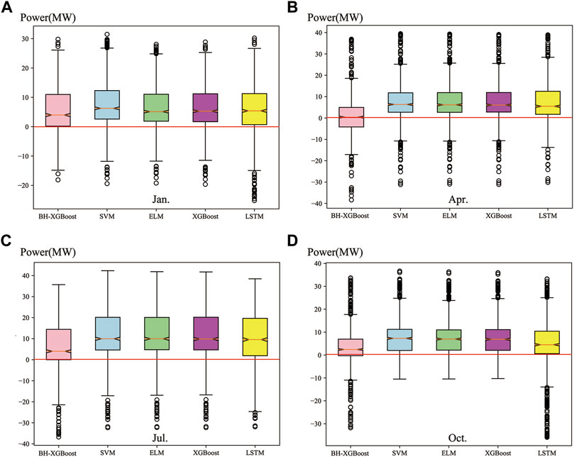
FIGURE 6. The residual boxplot of the result obtained by the different methods against the observation for different cases: (A) Jan., (B) Apr., (C)Jul., (D)Oct.

In order to verify the advantage of the proposed method, Figure 7 presents the residual distribution of the different methods for four different months. For all the cases, the kurtosis of the distribution curve for BH-XGBoost is lower than the other curves, and all the skewness of distribution curves is relatively positive. In Figures 7F,K, the residual distribution obtained by BH-XGBoost conforms to the normal distribution which means that the proposed algorithm has better robustness.

FIGURE 7

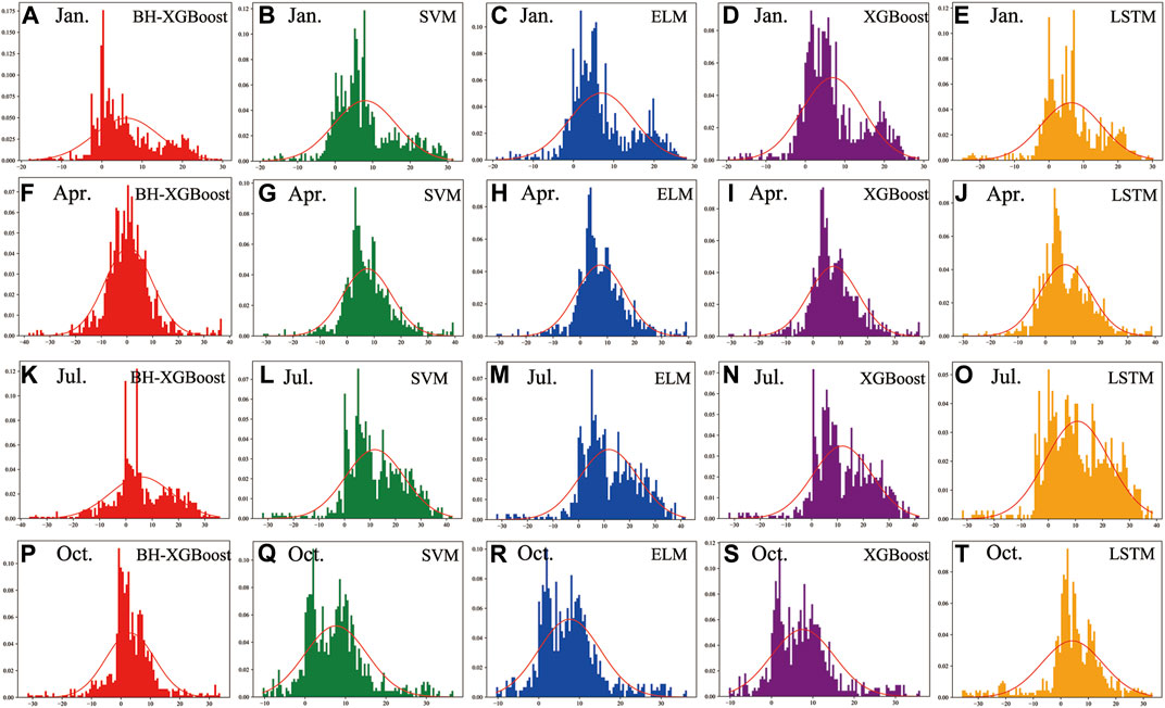
FIGURE 7. The residual distribution of the different methods for different cases: (A–E) for Jan., (F–J) for Apr., (K–O) for Jul., (P–T) for Oct.

5 Conclusion

A new short-term wind power forecast method based on XGBoost is explored in this article. The proposed method utilizes a Bayesian optimization hyperparameter, which can create the best-fit regression between the wind speed from WRF and the power from the target wind farm. To evaluate the new method, SVM, ELM, XGBoost and LSTM are employed to compare the performance of BH-XGBoost. For the case study results, the BH-XGBoost was significantly better than other methods. This method is reasonable because BH-XGBoost, as hyperparameter optimization based on Bayesian, yields the best-fit regression while other methods do not optimize hyperparameters according to the characteristics of the target wind farm.

Compared with other methods, the proposed method can effectively improve the accuracy of wind power forecasting especially in the cases of wind ramp events caused by extreme weather conditions and low wind speed ranges. For all the cases, the results of the RMSE, MAE and R-square show that the proposed method outperforms other methods. As expected, when the physics are spatially coherent, the methods work well, but when local spatiotemporal scale strong convective weather conditions dominate, the methods do not work. Thus, in future research, we will improve and test the BH-XGBoost method over more data and regions by integrating more meteorological elements, mainly when extreme events occur.

Data Availability Statement

The original contributions presented in the study are included in the article/Supplementary Material, further inquiries can be directed to the corresponding author.

Author Contributions

XX and XG contributed to the conception and design of the study. XW and RZ organized the database. PZ performed the statistical analysis. XX wrote the first draft of the manuscript. All authors contributed to manuscript revision, read, and approved the submitted version.

Funding

This research was partially supported by the Natural Science Foundation of Jiangsu Province under Grant no. BK20210661; Foundation of Jiangsu Rail Transit Industry Development Collaborative Innovation Base under Grant no. GCXC2105; Foundation of Collaborative Innovation Center on High-speed Rail Safety of Ministry of Education under Grant no. GTAQ2021001.

Conflict of Interest

Authors XX and RZ are employed by Nanjing University of Information Science and Technology, authors XG and PZ are employed by Hangzhou Dianzi University, author XW is employed by Guohua (Hami) New Energy Co., Ltd.

The remaining authors declare that the research was conducted in the absence of any commercial or financial relationships that could be construed as a potential conflict of interest.

Publisher’s Note

All claims expressed in this article are solely those of the authors and do not necessarily represent those of their affiliated organizations, or those of the publisher, the editors and the reviewers. Any product that may be evaluated in this article, or claim that may be made by its manufacturer, is not guaranteed or endorsed by the publisher.

References

Han, L., Romero, C. E., Wang, X., and Shi, L. (2018). Economic Dispatch Considering the Wind Power Forecast Error. IET Gener. Transm. & Distrib. 12, 2861–2870. doi:10.1049/iet-gtd.2017.1638

CrossRef Full Text | Google Scholar

Hanifi, S., Liu, X., Lin, Z., and Lotfian, S. (2020). A Critical Review of Wind Power Forecasting Methods-Past, Present and Future. Energies 13, 3764. doi:10.3390/en13153764

CrossRef Full Text | Google Scholar

Hao, Y., and Tian, C. (2019). A Novel Two-Stage Forecasting Model Based on Error Factor and Ensemble Method for Multi-step Wind Power Forecasting. Appl. energy 238, 368–383. doi:10.1016/j.apenergy.2019.01.063

CrossRef Full Text | Google Scholar

Huang, H., Jia, R., Shi, X., Liang, J., and Dang, J. (2021). Feature Selection and Hyper Parameters Optimization for Short-Term Wind Power Forecast. Appl. Intell. 51, 6752–6770. doi:10.1007/s10489-021-02191-y

CrossRef Full Text | Google Scholar

Ju, Y., Sun, G., Chen, Q., Zhang, M., Zhu, H., and Rehman, M. U. (2019). A Model Combining Convolutional Neural Network and Lightgbm Algorithm for Ultra-short-term Wind Power Forecasting. Ieee Access 7, 28309–28318. doi:10.1109/access.2019.2901920

CrossRef Full Text | Google Scholar

Kotthoff, L., Thornton, C., Hoos, H. H., Hutter, F., and Leyton-Brown, K. (2019). “Auto-weka: Automatic Model Selection and Hyperparameter Optimization in Weka,” in Automated Machine Learning (Cham: Springer), 81–95. doi:10.1007/978-3-030-05318-5_4

CrossRef Full Text | Google Scholar

Kumar, D., Abhinav, R., and Pindoriya, N. (2020). “An Ensemble Model for Short-Term Wind Power Forecasting Using Deep Learning and Gradient Boosting Algorithms,” in 2020 21st National Power Systems Conference (NPSC) (Gandhinagar, India: IEEE), 1–6. doi:10.1109/npsc49263.2020.9331902

CrossRef Full Text | Google Scholar

Li, K., Huang, D., Tao, Z., Li, H., Xiong, H., and Du, Y. (2020a). “Short-term Wind Power Prediction Based on Integration of Feature Set Mining and Two-Stage Xgboost,” in The Purple Mountain Forum on Smart Grid Protection and Control (Berlin, Germany: Springer), 64–81.

Google Scholar

Li, L., Li, Y., Zhou, B., Wu, Q., Shen, X., Liu, H., et al. (2020b). An Adaptive Time-Resolution Method for Ultra-short-term Wind Power Prediction. Int. J. Electr. Power & Energy Syst. 118, 105814. doi:10.1016/j.ijepes.2019.105814

CrossRef Full Text | Google Scholar

Liu, L., Ji, T., Li, M., Chen, Z., and Wu, Q. (2018). Short-term Local Prediction of Wind Speed and Wind Power Based on Singular Spectrum Analysis and Locality-Sensitive Hashing. J. Mod. Power Syst. Clean. Energy 6, 317–329. doi:10.1007/s40565-018-0398-0

CrossRef Full Text | Google Scholar

Maldonado-Correa, J., Solano, J., and Rojas-Moncayo, M. (2021). Wind Power Forecasting: A Systematic Literature Review. Wind Eng. 45, 413–426. doi:10.1177/0309524x19891672

CrossRef Full Text | Google Scholar

Phan, Q.-T., Wu, Y.-K., and Phan, Q.-D. (2020). “A Comparative Analysis of Xgboost and Temporal Convolutional Network Models for Wind Power Forecasting,” in 2020 International Symposium on Computer, Consumer and Control (IS3C) (Taichung City, Taiwan: IEEE), 416–419. doi:10.1109/is3c50286.2020.00113

CrossRef Full Text | Google Scholar

Quan, H., Khosravi, A., Yang, D., and Srinivasan, D. (2019). A Survey of Computational Intelligence Techniques for Wind Power Uncertainty Quantification in Smart Grids. IEEE Trans. neural Netw. Learn. Syst. 31, 4582–4599.

PubMed Abstract | CrossRef Full Text | Google Scholar

Rodríguez, F., Florez-Tapia, A. M., Fontán, L., and Galarza, A. (2020). Very Short-Term Wind Power Density Forecasting through Artificial Neural Networks for Microgrid Control. Renew. energy 145, 1517–1527.

Google Scholar

Santhosh, M., Venkaiah, C., and Vinod Kumar, D. (2020). Current Advances and Approaches in Wind Speed and Wind Power Forecasting for Improved Renewable Energy Integration: A Review. Eng. Rep. 2, e12178. doi:10.1002/eng2.12178

CrossRef Full Text | Google Scholar

Sideratos, G., and Hatziargyriou, N. D. (2020). A Distributed Memory Rbf-Based Model for Variable Generation Forecasting. Int. J. Electr. Power & Energy Syst. 120, 106041. doi:10.1016/j.ijepes.2020.106041

CrossRef Full Text | Google Scholar

Tian, Z. (2021). A State-Of-The-Art Review on Wind Power Deterministic Prediction. Wind Eng. 45, 1374–1392. doi:10.1177/0309524x20941203

CrossRef Full Text | Google Scholar

Wang, C., Wang, H., Zhou, C., and Chen, H. (2021). Experiencethinking: Constrained Hyperparameter Optimization Based on Knowledge and Pruning. Knowledge-Based Syst. 223, 106602. doi:10.1016/j.knosys.2020.106602

CrossRef Full Text | Google Scholar

Wang, Y., Zhou, Z., Botterud, A., and Zhang, K. (2017). Optimal Wind Power Uncertainty Intervals for Electricity Market Operation. IEEE Trans. Sustain. Energy 9, 199–210.

Google Scholar

Yang, L., Li, Y., and Di, C. (2019). “Application of Xgboost in Identification of Power Quality Disturbance Source of Steady-State Disturbance Events,” in 2019 IEEE 9th International Conference on Electronics Information and Emergency Communication (ICEIEC) (Beijing, China: IEEE), 1–6. doi:10.1109/iceiec.2019.8784554

CrossRef Full Text | Google Scholar

Yoo, Y. (2019). Hyperparameter Optimization of Deep Neural Network Using Univariate Dynamic Encoding Algorithm for Searches. Knowledge-Based Syst. 178, 74–83. doi:10.1016/j.knosys.2019.04.019

CrossRef Full Text | Google Scholar

Zameer, A., Khan, A., and Javed, S. G. (2015). Machine Learning Based Short Term Wind Power Prediction Using a Hybrid Learning Model. Comput. Electr. Eng. 45, 122–133.

Google Scholar

Zhang, C., He, Y., Yuan, L., and Xiang, S. (2017). Capacity Prognostics of Lithium-Ion Batteries Using Emd Denoising and Multiple Kernel Rvm. IEEE Access 5, 12061–12070. doi:10.1109/access.2017.2716353

CrossRef Full Text | Google Scholar

Zhang, C., Zhao, S., and He, Y. (2021). An Integrated Method of the Future Capacity and Rul Prediction for Lithium-Ion Battery Pack. IEEE Trans. Veh. Technol. 71, 2601.

Google Scholar

Zheng, H., and Wu, Y. (2019). A Xgboost Model with Weather Similarity Analysis and Feature Engineering for Short-Term Wind Power Forecasting. Appl. Sci. 9, 3019. doi:10.3390/app9153019

CrossRef Full Text | Google Scholar

Zheng, H., Yuan, J., and Chen, L. (2017). Short-term Load Forecasting Using EMD-LSTM Neural Networks with a Xgboost Algorithm for Feature Importance Evaluation. Energies 10, 1168. doi:10.3390/en10081168

CrossRef Full Text | Google Scholar

Zhou, C., Tang, W., Tang, W., and Zhao, R. (2017). Optimal Consumption with Reference-Dependent Preferences in On-The-Job Search and Savings. J. Industrial Manag. Optim. 13, 505–529. doi:10.3934/jimo.2016029

CrossRef Full Text | Google Scholar