Numerical Analysis of the Condensing Steam Flow by Means of ANSYS Fluent and in-House Academic Codes With Respect to the Capacity for Thermodynamic Assessment

In this paper numerical analysis of the condensing steam flow in a converging-diverging nozzle is investigated. The ANSYS Fluent results are compared with the results of the in-house academic Computational fluid dynamics code with respect to the capacity for thermodynamic assessment. The “local” real gas equation of state is used as a mathematical complement of flow governing equations in the in-house code. In the Fluent code, the thermodynamic functions as well as the steam and water physical properties are calculated based on the IAPWS formulation with the use of the UDF. The condensation model with the Fuchs and Sutigin correction of the droplet growth equation and nucleation rate with the Kantrowitz correction is implemented in both CFD codes. The CFD results are compared with the obtained experimental data. The experiment was carried out using an in-house steam facility with a transonic steam tunnel. The investigated geometry is a converging-diverging nozzle as adopted under the International Wet Steam Experimental Project with the diverging section expansion rate of 3,000 s⁻¹ and the total throat height of 40 mm.

Introduction

A broad understanding of condensing steam flows in power and aircraft industry is very significant. Condensation is a physical phenomenon that transforms a gas phase into a liquid phase. It may begin with a sudden expansion combined with the acceleration of the flow from subsonic to supersonic conditions. It is a common way to utilize the Laval nozzle, which is a convergent-divergent nozzle (CD nozzle), to speed up the working gas to supersonic flow conditions. After passing through the sonic region, in the divergent part of the nozzle, steam is supercooled to such an extent that a rapid condensation occurs and releases a large amount of latent heat to the gas phase. The name of this phenomenon is homogeneous spontaneous condensation and it involves high flow losses. The phenomenon is undesirable but inevitable. The first people who performed complex 2D simulation for the condensing flows were Young and White, who investigated the sensitivity of spontaneous condensation process, such as the effect of nucleation rate on the droplet size (White and Young, 1993). Over the following years a significant effort was made to properly model condensing steam flows thanks to the works of Schnerr (Schnerr et al., 2000), Halama (Halama et al., 2004) and many other researchers (Zhang et al., 2019; Xu et al., 2020) from around the world. The issues related to condensing flows are still topical. A mathematical model was developed by Yang et al. (2017) to predict the spontaneous condensing process in supersonic flows which indicates a good agreement between numerical and experimental results. A CFD model was developed by Wen et al. (2019) for the condensing flow of CO₂ in a supersonic nozzle. The results of this study offer an efficient and environmentally friendly method to reduce CO₂ emissions in the environment, which is the condensation of CO₂ in supersonic flows. Cao et al. (2020) simulated the flow field in the last stage of the steam turbine under low flow-rate conditions using the wet steam model. They showed the effect of the vortex location on the droplet diameter. Ding et al. (2021) increased the simulation accuracy of the wet steam flow using a poly-dispersion model. They showed that it is possible to foresee energy dissipation and the droplet spectrum in turbines. Amiri Rad et al. (2014) simulated the wet steam flow in the convergent-divergent nozzle one-dimensionally. They investigated the effect of the boundary layer on the formation and growth of droplets using mathematical models and compared with the inviscid flow. They showed that the droplet radius increased by 3%, if the boundary layer was considered in the simulation. Zhang et al. (2020) approximated the Wilson point and temperature parameters appropriately for the condensing steam flows in the Moses-Stein nozzle. Ding et al. (2014); Ding et al. (2015) approximated the location of the Wilson point and the flow properties analytically using classical nucleation equations and Young’s droplet growth model. They used a Bakhtar nozzle in high pressure and a Wyslouzil nozzle in low pressure to validate the results. They showed that the analytical solution is in a good agreement the experimental results. Various researches in the last 3 decades have improved the CFD modelling accuracy of the condensing steam flows. They have mainly focused on modifying the nucleation rate equation, improving the droplet growth model and using more precise equations of state for steam. The overall goal is to bring computational results closer to experimental data.

Most of the published CFD results of the modelling of condensing steam flows in CD nozzles do not include the information regarding the enthalpy-entropy diagram of the expansion line in the nozzle centre line. The line includes all data that could be used to check the thermodynamic properties of the expanded gas. This study presents numerical investigations of condensing steam flows in a converging-diverging nozzle. The analysis is conducted by means of the ANSYS Fluent and the in-house academic CFD codes, using the RANS density-based method with the k-ω SST turbulence model, with respect to the capacity for thermodynamic assessment. The IWSEP CD nozzle was selected for the testing (Zhang et al., 2021).

Experimental Data

The experimental data were obtained from the facility at the Department of Power Engineering and Turbomachinery of the Silesian University of Technology (cf. Figure 1). The steam tunnel is fed with superheated steam from a boiler. The greatest mass flow rate of steam is around 3 kg/s. The superheated steam conditions are regulated by sliding pressure in the boiler and the desuperheater at the live steam pipeline. Upstream of the test section (6), the parameters are precisely controlled by a control valve 1) and an extra desuperheater 14) to ensure steam parameters that correspond to the low-pressure turbine stages. The total inlet absolute pressure ranges from 70 to 150 kPa(a) and the total temperature ranges from 70 to 150°C.

FIGURE 1

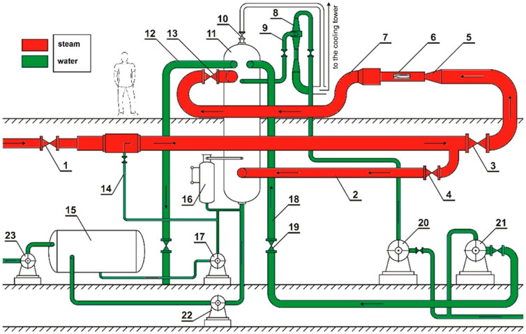
FIGURE 1. Steam tunnel facility (Dykas et al., 2018a) 1 - control valve; 2 - by-pass; 3 - stop gate valve; 4 - stop gate valve at by-pass; 5 - inlet nozzle; 6 - test section; 7 - outlet elbow; 8 - water injector; 9 - pipe; 10 - safety valve; 11 - condenser; 12 - suction line; 13 - throttle valve; 14 -desuperheater; 15 - condensate tank; 16 - control system of the condensate level; 17 - condensate pump; 18 - discharge line; 19 - stop valve; 20 - water injector pump; 21 - cooling water pump; 22 - condensate pump; 23 - pump.

In this paper, the investigated geometry is a convergent-divergent nozzle (CD nozzle) with a low expansion rate of 3,000 s⁻¹ and a throat height of 40 mm. This nozzle, which is the subject of investigation under the IWSEP, is made of aluminium (PA6) using CNC machining. As shown in Figure 2, a 110 mm-wide nozzle was installed in the test section of the steam tunnel located in the machinery hall of the Department of Power Engineering and Turbomachinery of the SUT. The test section with dimensions 1000 × 110 × 400mm, is made of stainless steel (1.4301) as well as the whole piping system.

FIGURE 2

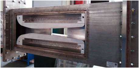
FIGURE 2. View of the investigated nozzle in the test section.

To measure the static pressure distribution at the bottom and the top wall, the measuring system includes 40 pressure sensors (20 measuring points on each wall). The measurement was carried out along the nozzle every 10 mm starting from position x = 0 m (nozzle throat). When all process parameters were completely stable, the static pressure values were averaged from samples of 5-s measurements. The static pressure distribution was collected by means of the Honeywell pressure sensors with a frequency of 400 Hz. The pressure pipes were purged before and after each measurement. To measure the liquid phase content, a light extinction measuring probe was used (Cai et al., 1992; Majkut et al., 2020). The measured data which are listed in Table 1, are for one set of inlet boundary conditions, including pressure, the droplet diameter and the liquid mass fraction (Zhang et al., 2021). The pressure data are given along the bottom wall, whereas the liquid phase was measured along the centre line of the nozzle. More details on the experimental campaigns for the IWSEP nozzle can be found in (Zhang et al., 2021).

TABLE 1

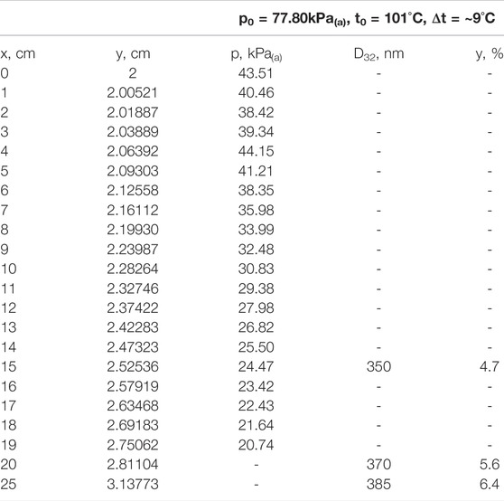
TABLE 1. IWSEP experimental data.

CFD Methods

Computational fluid dynamics (CFD) methods can be grouped into pressure-based and density-based solvers. For calculating the density in the compressible flow and in the density-based solver, the continuity equation is utilized and for calculating the pressure, the equation of state is used after the energy equation is solved. For calculating the pressure in pressure-based solvers, a pressure correction equation which results from combination of the continuity and momentum equations is solved. The density is then calculated from the equation of state. As it can be noticed, the equation of state plays a crucial role in both type of solvers. Both density- and pressure-based solvers are available in the Fluent software. The in-house CFD code is a density-based solver because historically these solvers have been mainly used for high-speed compressible flows. The in-house CFD code of the Department of Power Engineering and Turbomachinery of the SUT was developed over 25 years ago, before commercial CFD codes such as Fluent for instance, and was made available to academics. In both codes, the first-order upwind scheme with the AUSMD Riemann solver was set up in the calculations. The MUSCL scheme was used to increase the accuracy of spatial discretization. The numerical mesh was prepared in the ICEM CFD software according to the mesh-independence study previously made for this nozzle by Zhang et el. (Zhang et al., 2021).

In-House Code

The presented herein in-house CFD code has been elaborated over 20 years ago and has been successfully applied for CFD modelling of condensing steam flow for many technical applications, nozzle blade cascades, etc. (Dykas, 2001; Dykas et al., 2018a; Dykas et al., 2018b; Starzmann et al., 2018). In the in-house CFD code, the RANS method for the compressible steam flow was stated as:

$\frac{\partial }{\partial t}\mathrm{\rho }+\frac{\partial }{\partial x_j}\text{ρ}{\mathbf{v}}_{\mathbf{j}}=0(1)$

$\frac{\partial }{\partial t}\text{ρ}{\mathbf{v}}_{\mathbf{i}}+\frac{\partial }{\partial x_{ij}}\left(\text{ρ}{\mathbf{v}}_{\mathbf{i}}{\mathbf{v}}_{\mathbf{i}\mathbf{j}}+{\text{δ}}_{\text{i}\text{j}}\mathit{p}-{\mathbf{\tau }}_{\mathbf{i}\mathbf{j}}\right)=0(2)$

$\frac{\partial }{\partial t}\mathrm{\rho }E+\frac{\partial }{\partial x_j}\left({\mathbf{v}}_{\mathbf{j}}\text{ρ}E+{\mathbf{v}}_{\mathbf{j}}p\right)=\frac{\partial }{\partial x_j}\left(k_{eff}\frac{\partial }{\partial x_j}T+{\mathbf{\tau }}_{\mathbf{i}\mathbf{j}}{\mathbf{v}}_{\mathbf{j}} \right)(3)$

The continuity Eq. 1, the momentum Eq. 2 and the energy Eq. 3 are defined for a steam/water mixture, where $\text{ρ}$ is density, t is time, $v$ is the velocity vector, $\text{δ}$ is the Kronocker delta, p is pressure, $\tau$ is the stress tensor, E is total internal energy, $k_{\text{eff}}$ is effective conductivity, T is temperature. The total specific internal energy is calculated from the relation:

$E=h_{\mathrm{v}}\left(1-y_{\mathrm{hom}}\right)+{\mathrm{h}}_{\mathrm{l}}{y}_{\mathrm{hom}}-\frac{p}{\rho }+\frac{1}{2}{\mathbf{v}}_{\mathrm{j}},(4)$

where y_hom is the liquid mass fraction arising due to homogenous condensation and h_v and h_l are the specific enthalpy of vapour (steam) and water, respectively.

The “local” real gas equation of state is used in the in-house code as a mathematical closure of partial differential equations (Dykas, 2001). The purpose of using this equation is to make an equation as simple as possible, but very accurate at the same time. As the flow through the nozzle occurs in a bounded range of steam parameters, it is not necessary to use the equation of state covering the whole region of superheated steam. That’s why a simplified form of the real gas equation of state has been created.

The mathematical form of the used real gas equation of state 5) is similar to the virial equation of state with one virial coefficient.

$\frac{p}{\rho RT}=z\left(T,\rho \right)=A\left(T\right)+B\left(T\right)\rho (5)$

where

$A\left(T\right)=a_0+a_{1}T+a_2{T}^2,$

$B\left(T\right)=b_0+b_{1}T+b_2{T}^2.$

Coefficients a_0..2 and b_0..2 of polynomials A(T) and B(T) depend on temperature only and can be found by approximating the thermodynamic properties of steam given in the IAPWSIF′97. It can easily be noticed that this equation is represented by a relatively uncomplicated approximate surface (cf. Figure 3, Dykas, 2001).

FIGURE 3

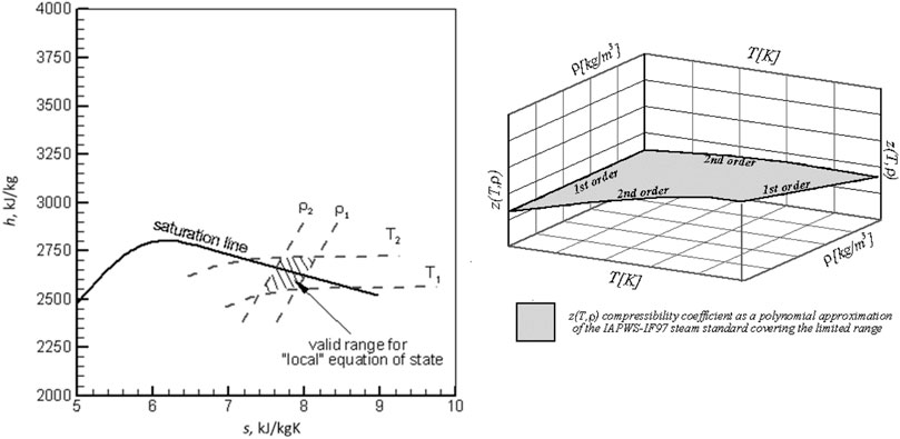
FIGURE 3. Mollier diagram of the “local” real gas equation of state near the saturation line.

Eq. 5 was named the ‘local’ equation of state (LEOS), as it can be used in a limited parameter range only. This equation can be applied to arbitrary real gases, not only to steam, and to the ideal gas assuming a₀ = 1 and a₁, a₂, b₀, b₁, b₂ = 0. The numerical algorithm for the RANS equations closed by the real gas equation of state is more complicated than the one for the ideal gas equation of state. It lengthens the computational time, but ensures accurate calculations of steam parameters.

LEOS coefficients are determined using a twenty-year-old in-house program, the graphic interface of which is currently not of the best quality (Figure 4). Figure 4 presents the numerical tool for determining the LEOS coefficients. The IAPWS formulations usually do not cover the supercooled steam region, i.e. the region much below the saturation line. Therefore, by building the “local” real gas equation of state, it is necessary to create a possibility of smooth extrapolation of the steam properties from the superheated region into the subcooled one. The extrapolation may proceed along isobars/isochores (Figure 4 left) or along isotherms (Figure 4 right). The red vertical line denotes the approximate expansion line in the nozzle, and the “+” sign symbolizes the location of total parameters. The black quadrangle shows the LEOS range for which the coefficients were determined. After many tests it was proved that assuming for the LEOS a range covering the supercooled region, the determined real gas equation of state for steam gave incorrect results in CFD modelling. This is probably due to exceeding the range of the IAWPS formulation for the metastable region.

FIGURE 4

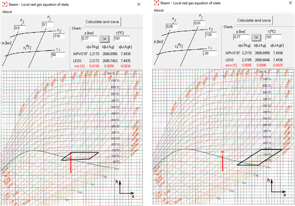
FIGURE 4. Parameter ranges for which the coefficients for the local equation of state were determined; left–pressure/density extrapolation into the supercooled region (LEOS 1), right–temperature extrapolation into the supercooled region (LEOS 2).

ANSYS Fluent

In the case of the Fluent code, the energy equation has the following form:

$\frac{\partial }{\partial t}\mathrm{\rho }E+\frac{\partial }{\partial x_{\mathrm{j}}}\left({\mathbf{v}}_{\mathbf{j}}\mathrm{\rho }E+{\mathbf{v}}_{\mathbf{j}}p\right)=\frac{\partial }{\partial x_{\mathrm{j}}}\left(k_{eff}\frac{\partial }{\partial x_{\mathrm{j}}}T+{\mathbf{\tau }}_{\text{i}\text{j}}{\mathbf{v}}_{\mathbf{j}} \right)+S_{\mathrm{E}}(6)$

where S_E is the source term due to homogeneous condensation

$S_{\text{E}}=S_{{\text{y}}_{\text{hom}}}.\left(h_{\text{v}}-h_{\text{l}}\right). (7)$

The physical properties of steam and water, i.e., saturation temperature, saturation pressure, latent heat, specific heat, thermal conductivity, viscosity and water density are computed based on the IAPWS relations. They are computed interactively in an external code and introduced to the ANSYS Fluent code by means of UDFs.

Condensation Model

It is necessary to consider another transport equations to model the phase change due to homogeneous condensation. Partial differential equations (PDEs) express the number of droplets per kilogram (n), created due to the nucleation process, and the liquid mass fraction (y), due to homogeneous condensation (hom). The additional transport equations which are implemented in the in-house CFD code (Dykas et al., 2018a; Dykas et al., 2018b) and in the ANSYS Fluent software (Wiśniewski et al., 2020) take the following form:

$\frac{\partial \mathrm{\rho }{y}_{\mathrm{hom}}}{\partial t}+\frac{\partial }{\partial x_{\mathrm{j}}}\left(\text{ρ}{\mathbf{v}}_{\mathbf{j}}{\text{y}}_{\mathrm{hom}}\right)=S_{{\text{y}}_{\mathrm{hom}}}(8)$

$\frac{\partial \mathrm{\rho }{n}_{\mathrm{hom}}}{\partial t}+\frac{\partial }{\partial x_{\mathrm{j}}}\left(\text{ρ}{\mathbf{v}}_{\mathbf{j}}{\text{n}}_{\mathrm{hom}}\right)=S_{{\text{n}}_{\mathrm{hom}}}(9)$

where S represents the source term: for —the source of mass of the condensed liquid due to homogenous condensation, for Eq. 9 – the source of droplets per kilogram of steam generated due to the nucleation process. The source terms are defined by the following formulae:

$S_{{\text{y}}_{\text{hom}}}=\frac{4}{3}{\text{πρρ}}_{\text{l}}{r}^{\text{∗}3}{J}_{\text{hom}}+4{\text{πρρ}}_l{n}_{\text{hom}}{r}_{\mathrm{hom}}^2\frac{\text{d}{r}_{\text{hom}}}{\text{d}t}(10)$

$S_{{\text{n}}_{\text{hom}}}=\text{ρ}{J}_{\text{hom}}(11)$

where J is the nucleation rate presenting the number of nuclei with critical radius r^* formed in 1 kg of moist air in one second; r is the droplet radius, which is calculated based on the water mass fraction and the number of droplets:

$r={\left(\frac{3y_{hom}}{4{\text{πρ}}_{\text{l}}{n}_{hom}}\right)}^{1/3}(12)$

It should be noted that in the case of heterogeneous condensation due to the presence of external nuclei, the droplet radius also accounts for the radius of the suspended particle.

The homogeneous condensation process is triggered by spontaneous nucleation, whereby nuclei, reaching the critical radius, form in the fluid due to rapid supercooling. In this model, the critical radius was based on the Kelvin equation:

$r^{\text{∗}}=\frac{2\text{σ}}{{\text{ρ}}_{\text{l}}{R}_{\text{v}}{T}_{\text{v}}\ln \left(\text{S}\right)}(13)$

where $\text{σ}$ is the steam surface tension, $R_v$ is the individual gas constant, $T_v$ is the steam temperature and $S=p_v/p_s$ is supersaturation, the ratio of steam partial pressure to saturation pressure. Assuming an equilibrium distribution of motionless clusters multiplied by the collision rate based on the kinetic theory of gases, the Volmer equation is formulated to describe the formation of condensation nuclei in 1 kg of moist air in one second:

$J_{\mathrm{hom}}=C\sqrt{\frac{2\sigma }{\mathrm{\pi }{m}_{\mathrm{v}}^3}}\frac{{\mathrm{\rho }}_v}{{\mathrm{\rho }}_l}{e}^{\left(-\frac{4\mathrm{\pi }{r}^{\ast 2}\sigma }{3k{T}_v}\right)}(14)$

where C is the Kantrowitz correction factor (Kantrowitz, 1951) defined as:

$C=\frac{{\alpha }_c}{1+\frac{2\left(\text{γ}-1\right)}{\left(\text{γ}+1\right)}\frac{(h_v-h_l)}{R_v{T}_v}\left(\frac{(h_v-h_l)}{R_v{T}_v}-\frac{1}{2}\right)}(15)$

where $\text{γ}$ stands for the ratio of specific heat capacities, $m_v$ is the mass of one molecule, ${\rho }_l$ is the liquid density at temperature $T_v$, and ${\alpha }_c$ represents the condensation coefficient, which is equal to one. In the non-isothermal Kantrowitz correction, it was assumed that all growing droplets have the same excess temperature. In the presence of a large volume of the gas phase such as moist air, as the collisions of condensed molecules with inert gas molecules are much more common than those with condensed droplets, the isothermal assumption is justified. . Finally, it reduces nucleation by a factor of 50–100.

Once a cluster of nuclei is formed in supercooled vapour, their further growth can be described as a function of supersaturation, the droplet size and thermodynamic properties. According to the gas dynamics theory, the collision frequency of steam molecules with condensed nuclei is associated with the mean free path of the steam molecules and the radius of water droplets. The larger the Knudsen number (Kn), the smaller the diameter of the droplet. The equation for calculating Kn is:

$Kn=\frac{l_S}{2r}=\frac{\frac{{\text{μ}}_l}{p}\sqrt{\frac{\text{π}RT}{2}}}{2r}(16)$

where l_s is the mean free path of the steam molecule, μ is dynamic viscosity of moist air, T is temperature, R is the gas constant; p is the moist air pressure, r is the droplet radius. If Kn < 0.01, the droplet growth process can be described as a continuous flow region. If Kn > 4.5, the droplet growth is governed by the free molecular flow. If 0.01 ≤ Kn ≤ 4.5, the transition region is the case.

The continuous model is derived for very large droplets. Considering that the droplet growth rate model should be applicable for small droplets, several models which take account of the Knudsen number were derived. Heiler (Heiler, 1999) was the first to use the Fuchs-Sutugin difference formula to correct the Gyarmathy continuous model:

$\frac{\text{d}r}{\text{d}t}=\frac{1}{{\text{ρ}}_l}\cdot \frac{\left(1+2Kn \right)\left(1-\frac{r^{\ast }}{r}\right)}{r\left(1+3.42Kn+5.32K{n}^2\right)}\cdot \left(\frac{{\text{λ}}_v{R}_v{T}_v^2}{{\left(h_v-h_l\right)}^2}\right)\cdot \ln \left(S\right)(17)$

In the presented codes, the condensation model with the Fuchs-Sutugin correction and the nucleation rate with the Kantrowitz correction are implemented.

Results and Discussion

A structured mesh was used for the analysed nozzle. It was generated using the ICEM CFD software (cf. Figure 5). The calculations were performed with the in-house CFD code and the ANSYS FLUENT 2019R3 package with the UDF to cope with additional transport equations and the IAPWS relations. Both codes operated on the same numerical mesh. The steam properties were taken from the IAPWS97 formulation. The k-ω SST turbulence model was applied in both codes. After the mesh-independence test (Zhang et al., 2021), the number of the mesh nodes was adopted as 81 × 301 × 3 keeping the y + value of 1. The nozzle walls are treated as no-slip, smooth and adiabatic. The total pressure and the total temperature values together with the turbulent intensity of 5% were set at the inlet. The values of the inlet boundary conditions are listed in Table 1. The boundary condition for the nozzle outlet was supersonic, and symmetry was assumed for the lateral walls.

FIGURE 5

FIGURE 5. Computational domain of the IWSEP nozzle.

Studying the results of the International Wet Steam Modelling Project (IWSMP) (Starzmann et al., 2018) obtained worldwide from research on condensing steam flows in nozzles, it can be noticed that they were compared for static pressure and the mean droplet radius only. The explanation was that only these values were available from experimental research. True, direct measurements of enthalpy, entropy or efficiency are impossible. It is puzzling though that the numerical results obtained for all used numerical codes with different condensation models and gas equations of state more or less coincide with experimental data. This was possible because condensation models include many correction factors which can be easily used to calibrate the numerical result to get satisfactory agreement with experimental data. Presenting the enthalpy-entropy diagram of the expansion line in nozzles together with isentropic efficiency would verify the usefulness of the applied numerical codes. After all, the CFD codes modelling the condensing steam flow are intended to determine the losses related to the appearance and presence of the liquid phase in the flow, and this cannot be done without proper determination of the thermodynamic parameters of steam.

The CFD results obtained by means of the two codes were compared with experimental data with respect to the static pressure distribution along the nozzle bottom wall and the wetness mass fraction, as well as the droplet diameter along the nozzle centre line (Zhang et al., 2021). Figure 6 shows the comparison of the static pressure distribution along the bottom wall of the nozzle. The results obtained using the in-house CFD code with two local equations of state (LEOS1 and LEOS2) and those produced by the ANSYS Fluent package were compared with experimental data. In both CFD codes the location of the onset of condensation is very similar and agrees with the experiment. However, for the ANSYS Fluent results the intensity of the condensation wave is much lower compared to the in-house CFD code and the experiment. However, for assessing the quality of an individual CFD solution more experimental data is needed.

FIGURE 6

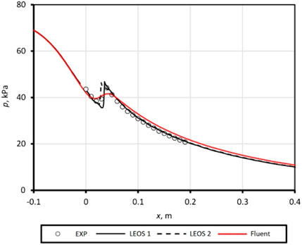
FIGURE 6. Comparison of static pressure along the nozzle bottom wall.

Figure 7 gathers the static pressure maps for the numerical results produced by the two CFD codes. In spite of the same numerical mesh and similar resolution of spatial discretization (MUSCL method), it is observed that the quality of the ASNYS Fluent results is poorer. In order to achieve similar spatial resolution, the number of the mesh nodes in the X direction in the numerical mesh for the ANSYS Fluent code should be at least twice higher.

FIGURE 7

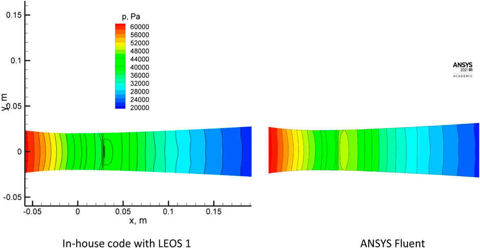
FIGURE 7. Static pressure maps.

Good agreement can be seen between CFD results and experimental data in relation to the mean droplet diameter (cf. Figure 8) and the wetness mass fraction (cf. Figure 9). However, there is a noticeable difference in the case of the mean droplet diameter between the ANSYS Fluent results and the results from the in-house CFD code obtained for two local equations of state, the LEOS1 and the LEOS2. The best agreement between the CFD results and the experimental data can be observed for the in-house code with the LEOS2, i.e. the local equation of state that extrapolates the gas properties into the wet steam region along isotherms. This is probably caused by a better prediction of the gas phase properties in the wet steam region. So far, all CFD results have demonstrated satisfactory agreement with the experiment regarding static pressure and wetness mass fraction distributions. One visible difference is in the mean droplet diameter, what is difficult to explain It just shows how sensitive is the solution to the gas phase thermodynamic properties.

FIGURE 8

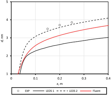
FIGURE 8. Comparison of the mean droplet diameter along the nozzle centre line.

FIGURE 9

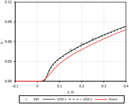
FIGURE 9. Comparison of the wetness mass fraction along the nozzle centre line.

Comparing the other thermodynamic parameters, it is found that without an accurate real gas equation of state for the mathematical closure of the steam flow governing equations, huge differences arise in temperature, entropy, enthalpy, etc.

It can be seen that even slight differences between the LEOS1 and the LEOS2 cause significant differences in the results. It should also be remembered that to model the wet steam flow, the gaseous phase properties are needed, and these are normally not available in the IAPWS data because much below the saturation line their experimental verification is difficult.

Figure 10 shows small differences in the static temperature distribution along the nozzle centre line between the CFD in-house code with the LEOS1 and the LEOS2. After the condensation onset, the static temperature obtained from the ANSYS Fluent software differs from the in-house code results significantly. Before the onset of condensation, all static temperature distributions are very much the same.

FIGURE 10

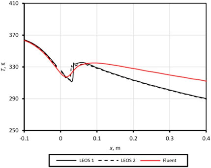
FIGURE 10. Comparison of static temperature along the nozzle centre line.

Similarly, for the enthalpy-entropy diagram of the expansion line (cf. Figure 11), all results are very similar until the condensation wave. After the condensation process, small differences are observed for the in-house CFD code with the LEOS1 and the LEOS2. For the ANSYS Fluent results, after the onset of condensation a very high increase in specific entropy can be observed. This leads to the expansion line of abnormal deviation to the right, out of the specific entropy range marked in Figure 11.

FIGURE 11

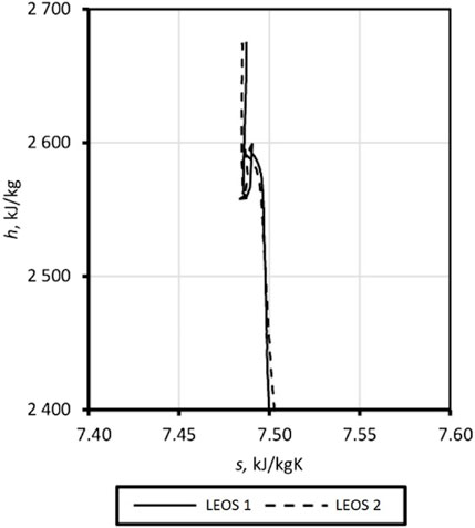
FIGURE 11. Comparison of the enthalpy-entropy diagram of the expansion line along the nozzle centre line.

Finally, the Ansys Fluent CFD results cannot be used to calculate the isentropic efficiency of the expansion process in the nozzle from the equation

$\eta =\frac{h_1-h_2}{h_1-h_2+T_{2}d{s}_{1-2}}(18)$

(where subscripts 1 and 2 denote the nozzle inlet and outlet, respectively) because the isentropic efficiency value would then be about 0.3 (30%). Considering the results from the in-house CFD code, the calculated isentropic efficiency is 0.984 for the LEOS1 and 0.980 for the LEOS2. The losses due to the homogeneous condensation process in the nozzle usually amount to a few per cent.

Summary and Conclusion

This paper presents a comparison of the CFD results of the condensing steam flow through the IWSEP nozzle. The flow was modelled numerically using an in-house CFD code and the ANSYS Fluent software. The numerical results were compared with experimental data for one set of inlet boundary conditions. The aim of the comparison was to find the differences between the two CFD codes with regard to the thermodynamic parameters which are usually not taken into account by researchers working on this problem. The two quantities which are usually taken into consideration in the analysis of condensing steam flows are the static pressure distribution and the mean droplet diameter. In our opinion, after many years of dealing with condensation models in two-phase flows, the first and the most important thing is to be sure that all thermodynamic parameters for the gaseous phase are calculated properly.

Based on the analysis of the performed comparison, the following remarks can be made:

• The in-house CFD code uses the real gas equation of state to solve the governing equations for the compressible flow.

• In the ANSYS Fluent software it was difficult to implement the real gas equation of state to solve the governing equations. The steam properties were computed interactively in an external code and introduced into the ANSYS Fluent code using the UDF.

• Both CFD codes showed good agreement with the experiment in relation to the static pressure distribution and the wetness mass fraction.

• The mean droplet diameter values agree with the experiment very well for the results obtained using the in-house code with the LEOS2. This proves that the influence of the gas equation of state on the results is very strong.

• Using the in-house CFD code, the expansion line for the condensing steam flow in the nozzle can be drawn correctly, which was not possible using the ANSYS Fluent software.

• The isentropic efficiencies calculated from the results of the in-house CFD code have realistic and expected values.

Data Availability Statement

The original contributions presented in the study are included in the article/supplementary material, further inquiries can be directed to the corresponding author.

Author Contributions

SS, supervision, writing original draft, review; editing. MM, carried out the experiment and provided the experimental data. SD, carried out the experiment and provided the experimental data, CFD calculations, revision. PW, CFD calculations. KS, carried out the experiment and provided the experimental data. XC, provided the experimental equipment, and guided the experiment. GZ, CFD support. All the authors were responsible for writing the paper and have given approval to the final version of the manuscript.

Funding

Research reported in this publication was supported by the National Science Centre under number 2020/37/B/ST8/02369, and by statutory research funds for young scientists.

Conflict of Interest

The authors declare that the research was conducted in the absence of any commercial or financial relationships that could be construed as a potential conflict of interest.

Publisher’s Note

All claims expressed in this article are solely those of the authors and do not necessarily represent those of their affiliated organizations, or those of the publisher, the editors and the reviewers. Any product that may be evaluated in this article, or claim that may be made by its manufacturer, is not guaranteed or endorsed by the publisher.

References

Amiri Rad, E., Mahpeykar, M. R., and Teymourtash, A. R. (2014). Analytic Investigation of the Effects of Condensation Shock on Turbulent Boundary Layer Parameters of Nucleating Flow in a Supersonic Convergent-Divergent Nozzle. J. Sci. Iran. 21 (5), 1709–1718.

Google Scholar

Cai, X., Wanc, L., Ouyang, X., and Pa, Y. (1992). A Novel Integrated Probe System for Measuring the Two Phase Wet Steam Flow in Steam Turbine. J. Eng. Thermophys. 22 (6), 52–57.

Google Scholar

Cao, L., Wang, J., Luo, H., Si, H., and Yang, R. (2020). Distribution of Condensation Droplets in the Last Stage of Steam Turbine under Small Flow Rate Condition. Appl. Therm. Eng. 181 (181), 116021. doi:10.1016/j.applthermaleng.2020.116021

CrossRef Full Text | Google Scholar

Ding, H., Tian, Y., Wen, C., Wang, C., and Sun, C. (2021). Polydispersed Droplet Spectrum and Exergy Analysis in Wet Steam Flows Using Method of Moments. J. Appl. Therm. Eng. 182, 116148. doi:10.1016/j.applthermaleng.2020.116148

CrossRef Full Text | Google Scholar

Ding, H., Wang, C., Wang, G., and Chen, C. (2015). Analytic Equations for the Wilson Point in High-Pressure Steam Flow through a Nozzle. Int. J. Heat Mass Transf. 91, 961–968. doi:10.1016/j.ijheatmasstransfer.2015.08.039

CrossRef Full Text | Google Scholar

Ding, H., Wang, C., and Zhao, Y. (2014). An Analytical Method for Wilson Point in Nozzle Flow with Homogeneous Nucleating. Int. J. Heat Mass Transf. 73, 586–594. doi:10.1016/j.ijheatmasstransfer.2014.02.036

CrossRef Full Text | Google Scholar

Dykas, S., Majkut, M., Smołka, K., and Strozik, M. (2018). Analysis of the Steam Condensing Flow in a Linear Blade Cascade. Proc. Institution Mech. Eng. Part A J. Power Energy 232 (5), 501–514. doi:10.1177/0957650917743365

CrossRef Full Text | Google Scholar

Dykas, S., Majkut, M., Smołka, K., and Strozik, M. (2018). Study of the Wet Steam Flow in the Blade Tip Rotor Linear Blade Cascade. Int. J. Heat Mass Transf. 120, 9–17. doi:10.1016/j.ijheatmasstransfer.2017.12.022

CrossRef Full Text | Google Scholar

Dykas, S. (2001). Numerical Calculation of the Condensing Steam Flow. Task Q. 5 (No 4), 519–535.

Google Scholar

Halama, J., Arts, T., and Fořt, J. (2004). Numerical Solution of Steady and Unsteady Transonic Flow in Turbine Cascades and Stages. Comput. Fluids 33, 729–740. doi:10.1016/j.compfluid.2003.05.003

CrossRef Full Text | Google Scholar

Heiler, M. (1999). Instationäre Phänomene in Homogen/Heterogen Kondensierenden Düsen und Turbinenströmungen. Germany: Universität Karlsruhe: Karlsruhe.

Google Scholar

Kantrowitz, A. (1951). Nucleation in Very Rapid Vapor Expansions. J. Chem. Phys. 19 (9), 1097–1100. doi:10.1063/1.1748482

CrossRef Full Text | Google Scholar

Majkut, M., Dykas, S., and Smołka, K. (2020). Light Extinction and Ultrasound Method in the Identification of Liquid Mass Fraction Content in Wet Steam. Archives Thermodyn. 41 (No. 4), 63–92. doi:10.24425/ather.2020.135854

CrossRef Full Text | Google Scholar

Schnerr, G. H., Heiler, M., and Winkler, G. (2000). 1. Transonic Nonequilibrium Two-phase Wake Flow in Axial Cascades. J. Vis. 3 (3), 205. doi:10.1007/bf03181837

CrossRef Full Text | Google Scholar

Starzmann, J., Hughes, F. R., Schuster, S., White, A. J., Halama, J., Hric, V., et al. (2018). Results of the International Wet Steam Modeling Project. Proc. Institution Mech. Eng. Part A J. Power Energy 232 (5), 550–570. doi:10.1177/0957650918758779

CrossRef Full Text | Google Scholar

Wen, C., Karvounis, N., Walther, J. H., Yan, Y., Feng, Y., and Yang, Y. (2019). An Efficient Approach to Separate CO2 Using Supersonic Flows for Carbon Capture and Storage. Appl. Energy 238 (238), 311–319. doi:10.1016/j.apenergy.2019.01.062

CrossRef Full Text | Google Scholar

White, A. J., and Young, J. B. (1993). Time-marching Method for the Prediction of Two-Dimensional, Unsteadyflows of Condensing Steam. J. Propuls. Power 9 (4), 579–587. doi:10.2514/3.23661

CrossRef Full Text | Google Scholar

Wiśniewski, W., Dykas, S., Yamamoto, S., and Pritz, B. (2020). Numerical Approaches for Moist Air Condensing Flows Modelling in the. Int. J. Heat Mass Transf. 162, 120392. doi:10.1016/j.ijheatmasstransfer.2020.120392

CrossRef Full Text | Google Scholar

Xu, H., Wei, Z., and Zhonghe, H. (2020). Investigating the Dehumidification Characteristics of the Low-Pressure Stage with Blade Surface Heating. Appl. Therm. Eng. 164, 114538. doi:10.1016/j.applthermaleng.2019.114538

CrossRef Full Text | Google Scholar

Yang, Y., Walther, J. H., Yan, Y., and Wen, C. (2017). CFD Modeling of Condensation Process of Water Vapor in Supersonic Flows. Appl. Therm. Eng. 115 (115), 1357–1362. doi:10.1016/j.applthermaleng.2017.01.047

CrossRef Full Text | Google Scholar

Zhang, G., Dykas, S., Li, P., Li, H., and Wang, J. (2020). Accurate Condensing Steam Flow Modeling in the Ejector of the Solar-Driven Refrigeration System. Energy 212, 118690. doi:10.1016/j.energy.2020.118690

CrossRef Full Text | Google Scholar

Zhang, G., Dykas, S., Majkut, M., Smołka, K., and Cai, X. (2021). Experimental and Numerical Research on the Effect of the Inlet Steam Superheat Degree on the Spontaneous Condensation in the IWSEP Nozzle. Int. J. Heat Mass Transf. 165, 120654. doi:10.1016/j.ijheatmasstransfer.2020.120654

CrossRef Full Text | Google Scholar

Zhang, G., Zhang, X., Wang, F., Wang, D., Jin, Z., and Zhou, Z. (2019). Numerical Investigation of Novel Dehumidification Strategies in Nuclear Plant Steam Turbine Based on the Modified Nucleation Model. Int. J. Multiph. Flow 120, 103083. doi:10.1016/j.ijmultiphaseflow.2019.103083

CrossRef Full Text | Google Scholar