 Chang Xie
 Li Zhou
 Tiecheng Wu
 Renwei Liu
 Sijie Zheng
 Vladimir G. Tsuprik
 Alexander Bekker
- 1School of Naval Architecture and Ocean Engineering, Jiangsu University of Science and Technology, Zhenjiang, China
- 2Nantong COSCO KHI Ship Engineering Co., Ltd., Nantong, China
- 3School of Ocean Engineering and Technology, Sun Yat-sen University, Zhuhai, China
- 4School of Engineering, Far Eastern Federal University, Vladivostok, Russia
The brash ice channel formed with icebreaker navigation is a normal working scenario for ice-going vessels. Therefore, it is necessary to study brash ice resistance in this condition. In this study, CFD and DEM coupling methods were adopted to investigate the resistance performance of a ship sailing in model-scaled brash ice fields, considering the collision force and friction resistance, among the brash ice, and the water resistance and hydrodynamic force of brash ice, which make up physical scenarios of navigation in the brash ice channel. To study the effect of aforementioned parameters on the average total resistance, the time step, iteration, and brash ice stiffness were analyzed; we found that a time step of 0.02 s, iteration of 10, and brash ice stiffness of 1000 N/m that showed better repeatability of the physical phenomenon, and it was used to reproduce working conditions created in the HSVA ice tank test. The error between the numerical simulation results and the test results is less than 5%, which shows the robustness of the present coupling strategy. Finally, the effects of ship–ice friction coefficient, ice thickness, ice shape, brash ice channel width, and ice concentration on the resistance of the ship were investigated and verified with the published results.
Introduction
With the Arctic route becoming more available, the number of ships navigating through the Arctic route is increasing. Icebreakers are needed to navigate the Arctic route for ships of low ice class, to form a brash ice channel. Therefore, it is significant to study the channel resistance of brash ice. The brash ice channel is characterized by the ice–water mixed multiphase flow. The resistance is usually evaluated by the empirical formula method, numerical simulation method, and ship model test method.
The most acceptable empirical formula method is the Finnish-Swedish Ice Class Rules (FSICR) based on the Baltic Sea ice conditions (Trafi, 2010; Trafi, 2011), and most classification societies use the FSICR assessment method. However, the brash ice resistance predicted by the Finnish-Swedish Ice Class Rules is usually higher than that of the ice tank test (Zhang et al., 2013; Jeong et al., 2017). To extend the FSICR brash ice channel resistance assessment method to the Arctic, Karulina et al (2019) proposed a computational model based on the FSICR method to estimate the ice resistance of ice-broken channels considering the special environment of the Arctic. There were still many factors not considered under the severe and moderate ice conditions. Dobrodeev and Sazonov (2019) established a theoretical model to calculate the resistance of the brash ice channel based on the real ship data and test data. The theoretical model was in good agreement with the ice tank test results.
The ship model test is the most acceptable method to evaluate the brash ice resistance, which can be divided into the refrigerated ice test in an ice tank and synthetic ice test in a conventional towing tank. The ice tank test is the closest method to the actual ice condition, but its cost is high. Cho et al. (2013) carried out a brash ice resistance test in a square ice tank at the Korea Research Institute of the Ship and Ocean Engineering (KRISO). Seong-YeobJeong et al. conducted a brash ice channel resistance test based on the Finnish Transport Safety Agency (2017) and Swedish Transport Agency (2011) in the KRISO ice tank. The IA ice class and IB ice class brash ice resistance tests were carried out in the ice tank, and the model test results were compared with the results of the FSICR formula (Jeong et al., 2017). In 2019, the effects of channel width, ice concentration, and ice thickness on the brash ice resistance in the ice tank were studied (Jeong and Kim, 2019). Zhou et al. (2019) carried out a brash ice test at the Aalto University Ice Tank in Finland to study the effects of ice thickness, speed, and heading angle on the brash ice channel resistance.
For scientific research institutes without an ice tank test, synthetic ice in the conventional towing tank is the alternative. Kim et al. (2013) carried out the brash ice resistance test in a conventional towing tank and compared the results with the brash ice resistance test in an ice tank. Guo et al. (2018a) carried out an experimental study on the brash ice channel resistance by using synthetic ice and studied the resistance characteristics under the conditions of four concentrations. Luo et al. (2018) used synthetic ice to investigate the interaction of ship–wave–ice in the periglacial area and the effects of wavelength, wave height, and ice concentration on the additional coupling resistance. Zong et al. (2020) also used synthetic ice to study the effects of different ice shapes, ice concentrations, and speed of brash ice on the brash ice resistance.
The ice–ship interaction model using numerical methods has been shown to be both efficient and accurate. The main numerical simulation methods used are the finite element method (FEM) and discrete element method (DEM). Kim et al. (2013) and Kim et al. (2014) simulated the brash ice resistance of 60–90% ice concentration using LS-DYNA software, and the results were compared with the synthetic ice test. Guo et al. (2018b) and Wang et al. (2020) also used LS-DYNA to simulate the brash ice resistance and compared it with the results of synthetic ice test. Yang et al. (2020) performed LS-DYNA brash ice resistance test simulation and compared it with the DuBrovin empirical formula. Kim et al. (2019) investigated brash ice resistance using ABAQUS and compared the results with ice tank test results. However, the finite element method cannot simulate the water resistance of the ship, which plays an important role in the real brash ice channel, also with expensive calculation cost; there are few studies on the simulation of the brash ice channel resistance by the finite element method. As for the discrete element method, Ji et al. (2013) used DEM to construct three-dimensional disk-shaped brash ice to simulate the interaction between ship and ice. Van Den Berg et al. (2019) studied the influence of floating ice shape on the ice load of vertical structures based on DEM. Based on the DEM of STAR CCM+ software, Luo et al. (2020) studied the simulation of the brash ice channel resistance of a bulk carrier and compared it with the ice tank test results. Guo et al. (2020) used STAR CCM+ software with DEM to study the resistance performance of a ship in an ice field with different ice concentrations and compared with the results of the synthetic model ice test. Huang et al. (2020) also used the DEM based on STAR CCM + software and compared it with the results of Guo’s synthetic model ice test. Polojärvi et al. (2021) used self-developed DEM to simulate the resistance performance of an actual ship in the floating ice field, and the simulation results were in good agreement with the actual ship navigation data. Yang et al. (2021) used self-developed DEM to simulate the brash ice resistance and to study the effects of brash ice shape, brash ice concentration, and friction coefficient of ship–ice on the brash ice resistance. In recent years, peridynamics has shown its advantage in simulation of the ship–ice interaction. Liu et al. (2018), Xue et al. (2019), Liu et al. (2020), and Liu et al. (2021) used peridynamics to simulate ship–ice collision and calculate the ice load and the ice destruction process during the ship–ice interaction. The influence of parameters such as time step, iterations, and brash ice stiffness is not investigated enough. Therefore, it is necessary to study the influence of parameters on the simulation results and propose a feasible numerical simulation strategy.
Following icebreaker navigation, the size of brash ice in the brash ice channel is small, and the possibility of the second break is low, so we can assume that the brash ice resistance caused by the second break can be ignored. Therefore, the resistance of polar ship in the brash ice channel mainly includes brash ice resistance and water resistance. The brash ice resistance is mainly caused by the collision of ship and ice and the friction of ship and ice. The brash ice resistance is affected by the viscosity of water by the hull movement, and the water resistance on both the ice and the hull cannot be ignored. Therefore, it is practical to use the viscous CFD and DEM coupling method to evaluate the resistance of the brash ice channel. In this study, the coupling method of CFD and DEM with STAR CCM+ software was used to analyze the influence of numerical simulation parameters, and the numerical simulation strategy was proposed. Then the simulation results were verified by the test results. Lastly, the effects of friction coefficient, ice thickness, ice shape, ice channel width and ice concentration on the resistance were analyzed.
Basic Formulation of the Numerical Model
In the numerical model, the fluid is an incompressible Newtonian fluid that satisfies the continuity and the momentum conservation equations, ignoring the heat exchange between the fluid and the discrete ice. For brash ice, the Lagrangian DEM was adopted.
CFD Numerical Model
The motion of an incompressible Newtonian fluid satisfies the continuity equation and conservation of momentum equation:
where ui and uj are the time mean of the velocity component (i, j = 1, 2, 3), P is the time mean of the pressure, ρ is the fluid density, μ is the dynamic viscosity coefficient, and Sj is the generalized source term of the momentum equation.
The governing equations are solved by the coupling of pressure, in which the convection term is discretized by the second-order upwind scheme and the dissipation term is discretized by the second-order central difference scheme. Considering the effect of wall shear force on the model, the SST (shear stress transport) k-ω model was adopted in order to simulate the strong counterpressure gradient flow, and Menter (1994) shows specific equations.
DEM Particle Motion Model
The DEM is a Lagrangian method, meaning that all particles in the computational domain are tracked by solving their trajectories explicitly. In the calculation process of the CFD and DEM coupling method, the interaction between ice particles and the interaction between ice particles and water is calculated by the discrete element method. The motion of DEM particles usually includes translation and rotation. Among them, the motion control equation based on Newton’s second law is as follows:
Momentum conservation equation (motion equation for DEM particle translation):
Angular momentum conservation equation (equation of motion for DEM particle rotation):
where mi, vi, and ωi represent the mass, velocity, and angular velocity of the particle i, respectively; Ii is the moment of inertia of the particle i; Fg is the gravity of the particle i; Ffluid is the force of the fluid on the particle i (including resistance, lift, additional mass force, and buoyancy); Fij is the collision force between the particle i and the particle j or the wall and other non-contact forces acting on the particle; and Tij is the contact moment, which is the torque generated by the contact force other than the particle gravity on the particle.
DEM Particle Contact Model
The Contact Model of Particle–Particle and Particle–Wall
In the simulation process, the contact and collision between particles and between particles and walls is the inevitable result of particle motion. Therefore, in terms of contact stress, this study chooses a computationally efficient and accurate linear spring contact model, which is a contact model based on the results of Cundall and Strack (1979). The contact force model is shown in Figure 1. Fn is the normal force, and Ft is the tangential force.
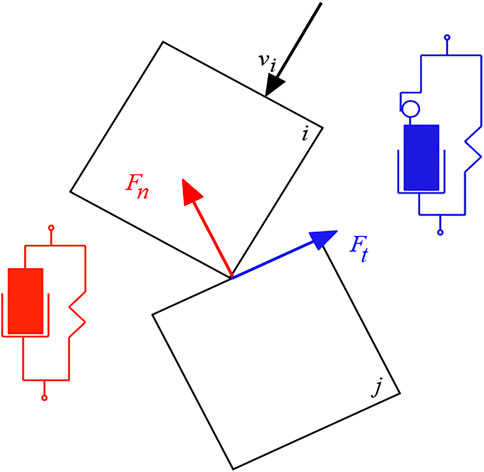
FIGURE 1. Spring-damper contact force model.
The contact force between two particles is:
where Fnij is the normal force and Ftij is the tangential force.
The normal force is:
where Kn is the normal spring stiffness, dn is the normal overlap of the contact point, Nn is the normal damping, and vn is the normal component of the sphere surface velocity at the contact point.
The expression for the tangential force is:
where Kt is the tangential spring stiffness, dt is the tangential overlap of the contact point, Nt is the tangential damping, vt is the tangential component of the sphere surface velocity at the contact point, and Cfs is the friction coefficient between particles.
The Interaction Model of Particle and Fluid
The interaction of DEM particles in the flow field mainly includes the buoyancy of the particle, the resistance of the flow field to the particle, the additional mass force, and the lift force on the particle. This study mainly calculates drag resistance, additional mass force, and pressure gradient force (including buoyancy effect). In the coupled calculation process, the moving DEM particles are subjected to drag resistance due to the existence of fluid viscosity, and the drag resistance of the particles is usually solved by the resistance coefficient. The solution of the DEM particle resistance coefficient in this study is achieved by the Haider and Levenspiel resistance coefficient (Haider and Levenspiel, 1989).
The drag resistance on the particle is as follows:
where Cd is the particle resistance coefficient, ρ is the fluid density, vs is the particle slip velocity (vs = vc−vd), vc is the water velocity, and vd is the particle velocity.
In this context, lift forces refer to mean forces normal to the particle velocity; they are not necessarily forces in the upward direction. Lift forces in statistical Lagrangian simulations can arise from particle shear only. This force applies to a particle moving relative to a fluid in which there is a velocity gradient in the fluid orthogonal to the relative motion.
where
The additional mass force on the particle is as follows:
where Cvm is the additional mass coefficient of the particle, Vp is the particle volume, ρ is the fluid density, and vp is the absolute velocity of the particle.
The DEM particles are subjected to the pressure gradient force in addition to fluid resistance and additional mass force. The expression of pressure gradient force on the particle is as follows:
where Vp is the volume of particles and
CFD-DEM-Coupled Numerical Model
The motion of incompressible Newtonian fluid satisfies continuity equation and momentum conservation equation (Norouzi et al., 2016):
where ρf is the density of fluid term, while εf is the volume fraction of the fluid term in the control volume. The relationship is that:
For the ship–ice–water coupling interaction, the average volume
where np is the number of discrete ice particles in each fluid control volume; uf is the dynamic viscous coefficient of the fluid;
The Configuration of Numerical Simulation
Research Object
The research object of this study was the ice-strengthened Panamax bulk carrier. The model test of the ship was carried out in the HSVA ice tank. The test items were the IA ice class and IB ice class brash ice channel test of the Finnish-Swedish Ice Class Rules. The brash ice channel was prepared according to guidelines set up by the Finnish Maritime Administration (FMA). The width of the brash ice channel was twice as wide as the beam of the ship model. The scale of the ship model was consistent with that of the Hamburg ice tank, and the scale ratio was 30.682, as shown in Figure 2.

FIGURE 2. Geometric ship model.
The main parameters of the ship model are shown in Table 1. For the ice tank test, different from the ship model test in a conventional towing tank, the similarity criteria include Froude number, Reynolds number, and Cauchy number. Since the Froude number and Reynolds number cannot be satisfied simultaneously in the model test and the influence of fluid viscosity on the test is relatively small, the Reynolds number similarity is usually ignored in the ice tank tests. In addition, the Cauchy law is usually considered in icebreaking and ice fracture problems. Therefore, the ice tank model test in HSVA considered the Cauchy law in the level ice model test and ignored the Cauchy law in the brash ice model test. Thus, in the present brash ice model tank test, the Froude number similarity is reserved. Therefore, the similarity criterion of numerical simulation is also Fourier number similarity.
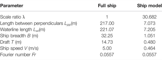
TABLE 1. Main parameters of the ship model.
Numerical Simulation Setup
A full ship model was used in the numerical simulation because of the asymmetric brash force on the ship. In accordance with the HSVA ice tank test conditions, the width of the brash ice channel was two times the ship breadth, and the calculated domain sizes of the brash ice channel were −2.5 Lpp ≤ x ≤ 3 Lpp, −2.0 Lpp ≤ y ≤ 2.0 Lpp, and −2.0 Lpp ≤ z ≤ 1.0 Lpp. The brash ice was arranged by an injector. The calculation domain of the brash ice channel is shown in Figure 3.
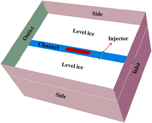
FIGURE 3. Computational domain setting of the brash ice channel.
The overall mesh of the computational domain is shown in Figure 4A. The boundary layer mesh adopted a prism layer mesh, and the volume mesh adopted the trimmed mesh. Meshes were refined on the hull surface, bow and stern, and free surface. To ensure reasonable simulation of the motion of brash ice in water and the ship–ice contact load, the hull surface mesh and free surface mesh of the ship–ice contact area were further refined, and the mesh of the brash ice movement region was smaller than the size of the brash ice, as shown in Figure 4B. Since the ship speed was very low, Fr number is only 0.0557. Therefore, to ensure the uniform transition of the boundary layer mesh to the body mesh, the value of wall Y+ of the hull surface below the waterline was less than 1, and the prism layer mesh before and after is shown in Figure 4C. The wall Y+ of the hull surface is shown in Figure 4D. In order to verify the mesh independence, based on the same mesh topology, three sets of grids were generated by adjusting the basic parameters of the trimmed mesh, which were the coarse, medium, and refine meshes.
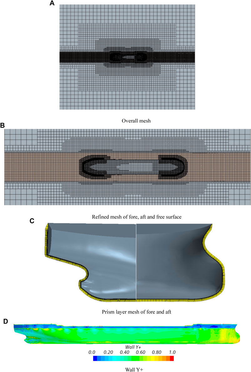
FIGURE 4. Computational domain mesh and wall Y+.
DEM Model of Brash Ice
The DEM brash ice particle model is the main factor affecting the brash ice resistance. References available mainly used the method of compounding brash ice particles to make brash ice models, and in this way, a combination of multiple basic spherical particles was used for a given geometric shape (Luo et al., 2020). The brash ice obtained by this method has two disadvantages: 1) the volume of combined brash ice does not match the actual, so the mass of combined brash ice is smaller than that of brash ice of the same size, and the resistance to the hull is also small. 2) Each combined brash ice consists of multiple or even dozens of spherical particles, resulting in a large number of DEM particles, and the calculation efficiency is reduced. Therefore, the straight brash ice geometry was adopted in this study, which could simulate the brash ice shape relatively realistically and reduce the number of DEM particles to improve the computational efficiency. The shape and size of the brash ice model were determined according to the brash ice distribution image of the HSVA ice tank test (as shown in Figures 5A,B), and the arrangement of the brash ice channel is shown in Figure 5C.
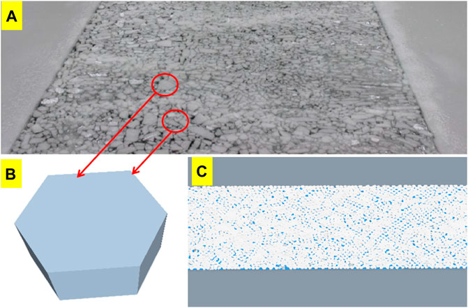
FIGURE 5. Shape of the brash ice model and the arrangement of the brash ice channel. (A) Brash ice distribution image of the HSVA ice tank test; (B) hexagonal brash ice model; (C) channel arranged by hexagonal brash ice.
In order to ensure that the numerical simulation was consistent with the ice tank test, the characteristic parameters of the brash ice model were set according to the data in the Hamburg ice tank test. The characteristic parameters of the model-scaled brash ice are shown in Table 2, and the target brash ice thickness is shown in Table 3. The length of brash ice models is set to about 50 mm, and the corresponding length of full-scale brash ice is about 1.5 m. But the actual length of brash ice is slightly different due to the influence of the injector. In the ice tank test, the ice thickness of FSICR IA and IB is selected as the test conditions according to the FSICR, and the corresponding target full-scale brash ice thickness is 1.42 and 1.22 m, and the corresponding target model-scaled brash ice thickness is 46.3 and 39.8 mm.
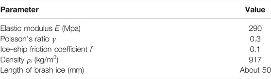
TABLE 2. Characteristic parameters of brash ice.
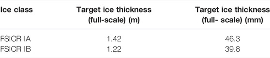
TABLE 3. Target brash ice thickness.
Numerical Parameters Determination
For numerical simulation, the mesh number has some influence on the results, so it is necessary to conduct mesh independence analysis to determine the appropriate grid. With time step ∆t elapsing, hull, brash ice, and water move toward each other, and the expression of the relative displacement ∆x is ∆x = U·∆t. The time step determines the intensity of the ship–ice collision. Therefore, it is necessary to study the effect of the time step on numerical simulation results. The iteration determines whether the calculation of the ship–ice collision converges, so it is necessary to study the effect of the iteration on the simulation results. The bending strength and compressive strength of the brash ice in the ice tank test are low, and the elastoplastic deformation of the brash ice will occur when it contacts the hull, while the elastoplasticity of the brash ice in the numerical simulation is defined by the stiffness, so it is necessary to study the effect of the brash ice stiffness on the simulation results. In this section, the ice thickness of 46.3 mm was used, and the effects of the time step, iteration, and brash ice stiffness on the simulation results were studied and compared with the experimental results, respectively. The resistance simulated with the present method was the average total resistance (including water resistance and brash ice resistance), and the average total resistance of the ice tank test results was 36.35 N.
Grid Independence
Time histories curves of the total resistance of the three grids are shown in Figure 6. It can be seen that the total resistance is strongly non-linear because of the randomness of ship–ice contact. With the increase of the grid number, the total resistance tends to increase. We can get the mean total resistance at the time of 50–75 s, and the mean total resistance results of three sets of grids are listed in Table 4. Three sets of grids number are 1.51 million, 3 million, and 4.12 million, corresponding to coarse mesh, medium mesh, and fine mesh, respectively. The difference between numerical simulation results and experimental results is within 6% with the increase of the grid number. So the numerical simulation results are not affected by the number of grids. Considering the efficiency and precision of numerical simulation, we chose a medium mesh as the basis of the progressive study.
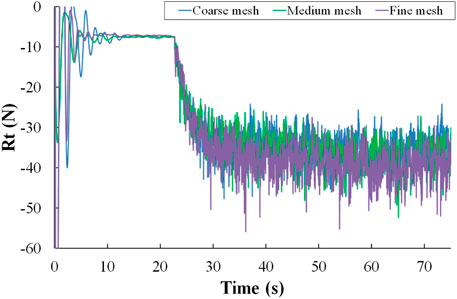
FIGURE 6. Time history curves of the total resistance of the three grids.
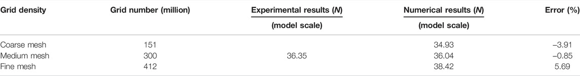
TABLE 4. Target brash ice thickness.
Time Step
The time step is usually determined according to the Courant number, which represents the relationship between the time step and the physical space. The Courant number CFL≈U·∆t/∆x, where ∆t is the time step and ∆x is the mesh size. According to the mesh size, the time step was usually set as 0.1 s. But for low Fr numbers, a smaller time step size is required.
To study the effect of time step on the simulation results, six groups of time steps were selected: 0.001, 0.01, 0.02, 0.05, 0.1, and 0.2 s. The relationship between the time step and the simulation results is shown in Figure 7A. It can find that the total resistance reaches its largest value as the time step is 0.001 s, while it changes from 0.01 to 0.02 s, the total resistance changes abruptly. When it changes from 0.02 to 0.2 s, the total resistance changes relatively gently, and the total resistance is the smallest as the time step size is 0.2 s. The reason is when the time step is smaller, the ship–ice collision is relatively moderate, the brash ice needs multiple time steps to complete the plastic deformation, and the ship–ice contact is more continuous. While the time step becomes larger, the process of plastic deformation cannot be completed within a one-time step, which leads to a decrease in the resistance of the brash ice. When the time step is 0.02 s, the total resistance is closer to the test results, and the Fr number is 0.0557. Therefore, 0.02 s is an appropriate time step to simulate the brash ice resistance more accurately.
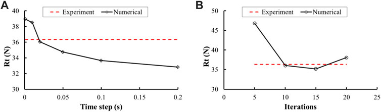
FIGURE 7. Influence of ship–ice friction coefficient and iterations.
Number of the Iteration
Numerical calculations for each time step require multiple iterations to obtain convergent results, so an appropriate iteration needs to be determined. In this section, we choose four sets of iterations: 5, 10, 15, and 20. The relationship between the iterations and the simulation results is shown in Figure 7B. It can be found that when the iterations are not less than 10, the error between the simulation results and the experimental results is small, and the calculation accuracy is high. Therefore, to balance the computational accuracy and computational efficiency, 10 is an appropriate iteration.
Brash Ice Stiffness
The stiffness of brash ice can show the elastoplasticity of brash ice. To make the actual mechanical properties of brash ice available, the stiffness should investigate further. In this work, five sets of brash ice stiffness including 10, 100, 1000, 10,000, and 100,000 N/m are analyzed. Figure 8 shows the effect of brash ice stiffness on the ship–ice collision. The relationship between the brash ice stiffness and the simulation results is shown in Figure 9A. It can be seen that when the stiffness of brash ice is 100,000 N/m, the total resistance is 31.15 N, 14.31% lower than the test result. It is because the ship–ice collision produces great elasticity just like the collision of two rigid bodies. At this moment, elasticity plays a leading role, so the brash ice quickly ricochets everywhere, as shown in Figure 8E, thus reducing the hull–ice contact time and resulting in reduced ice resistance. When the stiffness of brash ice is from 10,000 to 100 N/m, the elastic strength of ship–ice contact weakens and tends to the viscoelastic–plastic model of actual ship–ice collision. Therefore, the total resistance is closest to the test result, and the brash ice will not be bounced off, as shown in Figures 8B–D.When the stiffness of brash ice is reduced to 10 N/m, plasticity plays a leading role in ship–ice collision. The brash ice is like elastic ball, and the energy of ship–ice collision is absorbed by the plasticity of brash ice, resulting in a rapid decrease in ice resistance and a decrease in total resistance, as shown in Figure 8A. While the stiffness of the brash ice is 1000 N/m, the total resistance result is the closest to the test result. So the brash ice stiffness was chosen as 1000 N/m in the following investigation.

FIGURE 8. Influence of stiffness on the motion of brash ice.

FIGURE 9. Influence of stiffness and repeatability.
Robustness of the Simulation
According to the above research results, the time step of 0.02 s, the number of iterations of 10, and the brash ice stiffness of 1000 N/m were set in this section for further investigation. To verify the robustness of the numerical simulation, the aforementioned numerical simulation strategy was repeated 10 times. The numerical simulation results are shown in Figure 9B; the blue line is the mean total resistance of the 10 results. The results show that the total resistance fluctuates due to the randomness of the distribution of brash ice. The maximum value of the total resistance is 5.69% larger than the test result, the minimum value is 2.56% smaller than the test result, and the difference between the maximum value and the minimum value is 3N, which is 8.25% smaller than the test result. The average value of 10 times simulation results is 36.94 N, and the difference with the test results is 1.62%. Therefore, the numerical simulation strategy has good repeatability.
Numerical Simulation Validation
With simulation parameters determined in the previous section, the brash ice with different thicknesses were simulated and verified by experimental results in this section. The thickness of brash ice was 39.8 and 46.3 mm, and the speed of the brash ice was 0.464 m/s.
Analysis of Brash Ice Movement
Figure 10 shows the comparison between the simulation results and the ice tank test when the thickness of the brash ice model is 46.3 mm. When the ship model goes through the brash ice channel, the brash ice will be evacuated to both sides along with the bow of the ship (Figure 10A), leading to the accumulation of brash ice on both sides of the ship, and then push on the sides of the ship. It is the main reason for friction resistance between the ship and ice. The track of the brash ice among the stern is slightly closed after the ship passes through the brash ice channel (Figure 10B). The reason for this phenomenon is that the strength of the ice model using the similarity criterion is much smaller than that of the physical ice in the test, resulting in certain plasticity of the brash ice. The brash ice is pushed on both sides of the ship and plastic deformation occurs, so the brash ice in the stern track does not spread out due to the contact force between each other, and the stern track is slightly closed. In the numerical simulation, the brash ice is a polygonal solid, which will not be fractured or deformed but will be pushed below the ice surface and on the ice surface due to mutual extrusion when it is dislodged from the bow to both sides. (Figure 10C), but the effect of closing the ice channel in the stern of the ship is more obvious. Although the numerical simulation phenomenon and the ice tank test phenomenon are slightly different because of the different composition and performance, the overall phenomenon is in good agreement.
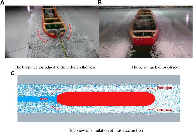
FIGURE 10. Comparison between numerical simulation and ice tank test when hi = 46.3 mm.
In the numerical simulation, the accumulation phenomenon and contact force of the brash ice on the bow are shown in Figure 11. Due to the influence of the bulbous bow and the large floating angle of the bow, the broken ice cannot slide downward along the hull and can only be discharged to both sides. In the process of displacement, it will accumulate in the bow and the shoulder of the bow, resulting in the contact force caused by the crushing of the ice and the hull. When the thickness of the brash ice increases from 39.8 to 46.3 mm, the brash ice is more difficult to be discharged to both sides, resulting in more serious accumulation and even the brash ice is squeezed onto or under the ice surface. So, 46.3 mm of brash ice induces a larger range of ship–ice contact force.

FIGURE 11. Brash ice accumulation and contact force on the bow.
Analysis of Resistance Results
Figure 12 shows the resistance–time curves of the ship in a brash ice channel when the ice thicknesses are hi = 39.8 mm and hi = 46.3 mm, where WaterRes is the water resistance, IceResX is the longitudinal brash ice resistance, and TotalResX is the total longitudinal resistance. The brash ice resistance components and the comparison with the test results are shown in Table 5.
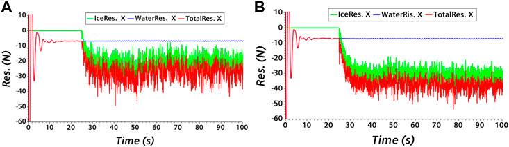
FIGURE 12. Time histories of resistance.
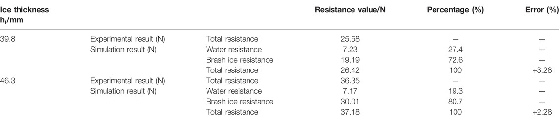
TABLE 5. Brash ice resistance components and comparison with the test results.
As shown in Figure 12, the hull began to contact the brash ice at time of 25 s, and the resistance of the brash ice began to gradually increase. With the randomness of ship–ice collisions and friction, the resistance of brash ice also fluctuates.
As shown in Table 5, the ice thickness increases from 39.8 to 46.3 mm, but the water resistance remains almost unchanged, and the brash ice resistance increases from 19.18 to 30.01 N, resulting in a decrease in the ratio of water resistance to the total resistance from 27.4 to 19.3%. The difference between the simulation results and the ice tank test results under the two ice thickness conditions is within 5%, indicating that the simulation results have good accuracy.
Numerical Simulation Applications
Brash ice parameters including the thickness and shape of brash ice, ship–ice friction coefficient, width of the brash ice channel, and concentration of the brash ice have an influence on the brash ice resistance. This section studied the influence of these parameters and compared with experimental results.
Influence of Ship–Ice Friction Coefficient
The ship–ice friction coefficient has an important influence on the ice resistance (Woolgar and Colbourne, 2010). Therefore, it is necessary to study the effect of the ship–ice friction coefficient on the average total resistance. The ice in this section is with a thickness of 46.3 mm, and the friction coefficient was changed from 0.01 to 0.02. Figure 13A shows the simulation results of the total resistance with the friction coefficient changed. When the ship–ice friction coefficient f is increased from 0.01 to 0.1, the total resistance increases almost linearly. When f is increased from 0.1 to 0.2, the total resistance gradually becomes larger. This result is well consistent with that obtained in Woolgar and Colbourne (2010) (see Figure 13B).
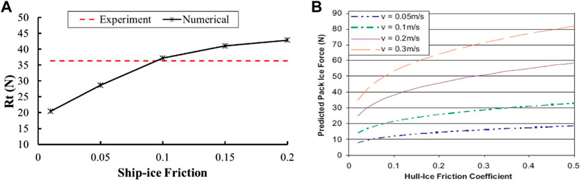
FIGURE 13. Influence of ship–ice friction coefficient on ice resistance.
Influence of Brash Ice Thickness
Ice thickness has an important influence on the resistance of brash ice. The numerical simulation settings remain the same as in the previous section, only the brash ice thickness was changed. Figure 14 shows the total resistance results for the thickness of the brash ice from 19.56 to 65.18 mm (the actual thickness of ice is from 0.6 to 2.0 m). As shown in Figure 14, the thickness of the brash ice has an important influence on the total resistance, and the total resistance is linear with the thickness of the brash ice. Since the thickness of the brash ice directly affects the mass of the ice, it affects the contact load between the ship and the ice and leads to the increase of the brash ice resistance. At the same time, due to the increase of the thickness of the brash ice, the volume of the brash ice in the channel increases, and the thickness of the brash ice that is dislodged to both sides of the ship increases, thus increasing the ship–ice contact area, which increases the ship–ice friction resistance, eventually leading to the increase of brash ice resistance.
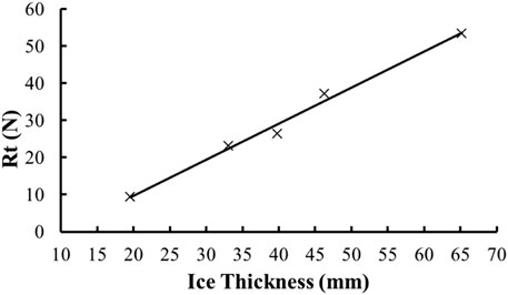
FIGURE 14. Influence of brash ice thickness on ice resistance.
Influence of Brash Ice Shape
In Section 3.3, we assumed that the hexagon was the shape of the brash ice in the actual channel, but the brash ice in the actual ice tank channel is composed of various irregular polygons. This section investigated the effect of other shapes of brash ice on resistance, including square, triangle, and circle. The numerical simulation conditions remained the same as in the previous section, only the shape of the brash ice was changed. Figures 15A–D show the numerical simulations of the ship interacting with different shapes of the brash ice.
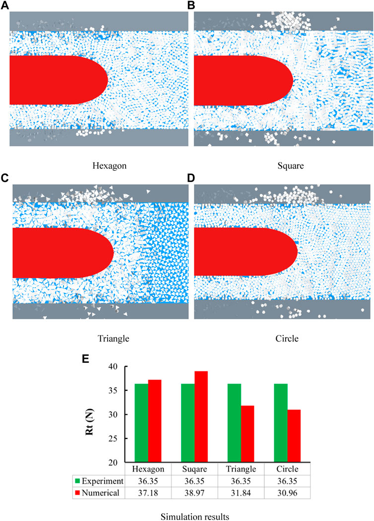
FIGURE 15. Numerical simulations with different shapes of brash ice and results.
Figure 15E shows the total resistance of the four shapes of brash ice. It is shown that the total resistance of the square brash ice is the largest, the total resistance of the hexagonal brash ice is the second, and the total resistance of the circular brash ice is the smallest. This is because the square has two pairs of parallel sides, and it is easier for the brash ice to form a dense accumulation on the bow and both sides, which makes it difficult for the brash ice to be discharged. At the same time, the square brash ice is more likely to increase the contact area with the hull, thereby resulting in an increase in the hull–ice frictional resistance. On the contrary, the circular fragments of brash ice are all tangent to each other, resulting in small ice–ice and ship–ice contact area, and small ship–ice contact force and friction resistance. This result is well consistent with that obtained in reference (Yang et al., 2021).
Influence of Channel Width
The width of the brash ice channel also has an important effect on the resistance of the icebreaker. The effect of the width of the brash ice channel on the resistance in the ice tank was done by Jeong and Kim (2019). In the present work, the width of the brash ice channel was changed from 1.2 times to 10.0 times the ship’s breadth. The numerical simulation conditions remained the same as in the previous section, only changed the width of the brash ice channel. Figure 16 shows the ship model in brash ice channels with eight different widths. In present work, the ship was fixed and the brash ice had a velocity moving toward to the ship. In Figure 16, we can find that when the brash ice channel is greater than eight times of the ship breadth, the overturning and translation of the brash ice on both sides of the brash ice field, and the brash ice tends to gather toward the center of the channel, which is different from the actual movement of the brash ice. However, due to the wide of the channel is large enough, the effect on the final result can be negligible. As the brash ice channel is less than eight times the ship breadth, the interaction between the brash ice and the water surface can also be ignored compared to ship–ice contact and ice–ice contact.

FIGURE 16. Numerical simulations with different widths of brash ice channels.
Figure 17A shows the numerical simulation results of the total resistance of brash ice channels with eight different widths. It can be seen that the total resistance decreases with the increase of the width of the brash ice channel, but when the width of the brash ice channel is greater than six times of the ship breadth, the total resistance decreases gradually. The reason is that as the width of the brash ice channel is greater than six times the ship breadth, the total resistance decreases gradually. When the width of the channel is less than two times the ship’s breadth, the total resistance is large. This is because the distance between the two sides of the ship and the ice is small, and the brash ice in the channel will be pushed to the narrow sides or even to the above or below the water surface, resulting in a thicker build-up of brash ice on the side of the ship, leading to the total resistance increased. Similar conclusions are reached by ice tank test in reference (Jeong and Kim, 2019), see Figure 17B.
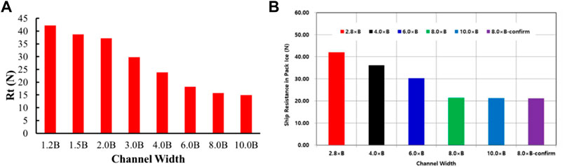
FIGURE 17. Influence of channel width on ice resistance.
Figure 18 show the transverse force of brash ice in 8 times channel width. The transverse force of the brash ice is positive to port and negative to starboard. As shown in Figure 18A, when the width of the brash ice channel is from 1.2 times to 2.0 times of the ship breadth, the pulsation amplitude of the transverse force–time curves of the brash ice is not significantly reduced, but the pulsation range is still large, which is from −20 to 30 N, the total transverse force of the brash ice is positive. It concluded that the transverse force of the brash ice points to the port side, which means that the accumulation of brash ice on the starboard side is heavier than that on the port side. When the width of the brash ice channel is from 2.0 times to 3.0 times of the ship breadth, the pulsation amplitude of the transverse curve is significantly reduced, and the total transverse force of the brash ice is negative when three times of the ship breadth. It concluded that the transverse force of the brash ice points to the starboard side, indicating that the accumulation of brash ice on the port side is more serious than that on the starboard side. The width of the brash ice channel ranges from 3.0 times to 4.0 times of the ship breadth, the total transverse force of the brash ice changes from a negative value to a positive value, and the pulsation range of the transverse force of the brash ice is −20 to 15 N. The pulsation amplitude of the transverse force curve is significantly reduced, when the width of the brash ice channel is from 6.0 times to 10.0 times of the ship breadth. The pulsation amplitude of the transverse force curve of the brash ice has been significantly weakened, and the pulsation range of the transverse force of the brash ice is −8–8 N. We find that the transverse force amplitude of brash ice is affected by the width of the brash ice channel. The smaller the width of the brash ice channel, the larger the transverse force amplitude and the greater the friction resistance.
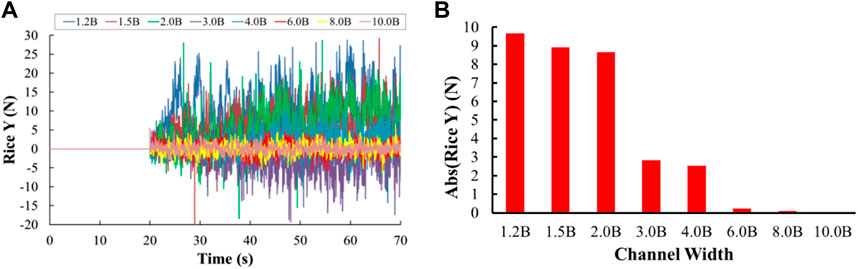
FIGURE 18. Transverse force.
As shown in Figure 18B, the absolute value of the average brash ice transverse force decreases with the decrease of the width of the brash ice channel. When the width of the brash ice channel is from 1.2 times to 2.0 times of ship breadth, the absolute value of the average transverse force decreases slightly from 9.68 to 8.66 N, and when the width of the brash ice channel is from two times to three times of ship breadth, the absolute value of the average transverse force of brash ice decreases greatly from 8.36 to 2.82 N, and the absolute value of the average transverse force of brash ice decreases slightly from 2.82 to 2.54 N when the width of the brash ice channel is from three times to four times of ship breadth. When the width of the brash ice channel is four times to six times of ship breadth, the absolute value of the average transverse force of the brash ice decreases obviously from 2.54 to 0.21 N, and when the width of the brash ice channel is 6.0 times to 10.0 times of ship breadth, the absolute value of the average transverse force of brash ice is very small, from 0.21 to 0.04 N.
Influence of Brash Ice Concentration
The concentration of brash ice is an important factor affecting the resistance of ships. The influence of the concentration of brash ice on the resistance was performed by the test method or numerical simulation methods (Woolgar and Colbourne, 2010; Cho et al., 2013; Kim et al., 2013; Kim et al., 2014; Guo et al., 2018a; Guo et al., 2018b; Jeong and Kim, 2019; Xue et al., 2020). According to the conclusion in channel width section, the brash ice channel of eight times of ship breadth was selected. The numerical simulation settings were kept consistent with channel width section using eight times of ship breadth, and only the brash ice concentration was changed. In the present work, four brash ice concentrations were simulated: 40, 50, 60, and 70%, and the brash ice channels of each concentration are shown in Figure 19.

FIGURE 19. Brash ice channels of different concentrations.
Figure 20A shows the simulation results of the total resistance of different widths of brash ice concentration. It can be seen that the total resistance increases with the concentration of the brash ice. From 40 to 70% brash ice concentration, total resistance has increased by 75%. Similar conclusions are reached by the ice tank test in reference (Cho et al., 2013), see Figure 20B.
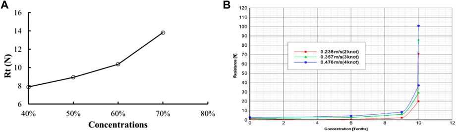
FIGURE 20. Influence of brash ice concentration on ice resistance.
Conclusion
In this study, a numerical simulation study of the resistance of the brash ice channel was investigated with the coupling method of CFD and DEM. The influence of numerical simulation parameters (including time step, iterations, and brash ice stiffness) was analyzed and compared with the experimental results. The effects of ship–ice friction coefficient, thickness of brash ice, brash ice shape, channel width, and brash ice concentration on resistance were analyzed. It can be concluded that:
(1) The numerical simulation parameters selected as the time step of 0.02 s, iterations of 10, and the brash ice stiffness of 1000 N/m can obtain reasonable results.
(2) The phenomenon of brash ice movement in the channel was in good agreement with the test results. The brash ice was dislodged from the bow to the sides of the ship, and the accumulation of the brash ice on the bow, the stern track of the brash ice, and the contact force between the hull and the brash ice could be captured.
(3) The precision of numerical simulation was high. As the ice thickness is 39.8 and 46.3 mm, the difference between the total resistance of the brash ice channel and the experimental results was 3.28 and 2.28%, respectively, and both of the errors were within 5%. Brash ice resistance accounted for more than 70% of the total resistance of the brash ice channel. The proportion of the brash ice resistance increased with the increase of ice thickness.
(4) The influence of the ship–ice friction coefficient on the total resistance is attenuated with the increase of the friction coefficient. The thickness of the brash ice had a linear relationship with the total resistance. The shape of the brash ice also affected the total resistance; the closer the opposite side of brash ice to the parallel, the greater the resistance, and the ice resistance is smaller to the smoother side of the brash ice. The larger the width of the brash ice channel, the smaller the total resistance. When the width of the brash ice channel was greater than eight times the ship breadth, the total resistance of the brash ice channel would not decrease with the increase of the channel width. The total resistance of the brash ice channel increased with the increase of the concentration of the brash ice.
Data Availability Statement
The original contributions presented in the study are included in the article/Supplementary Material, further inquiries can be directed to the corresponding author.
Author Contributions
LZ and TW contributed to the conception and design of the study. RL and SZ organized the database. CX performed the statistical analysis and wrote the first draft of the manuscript. All authors contributed to manuscript revision and read and approved the submitted version.
Funding
This work is funded by the National Key Research and Development Program (Grant No. 2022YFE0107000) and National Natural Science Foundation of China (Grant No. 52171259). The numerical study based on CFD and DEM coupling in this study has been guided by Yongze Xu and Wendong Liu from Siemens PLM Software, and we are deeply grateful for this.
Conflict of Interest
Author CX was employed by Nantong COSCO KHI Ship Engineering Co., Ltd.
The remaining authors declare that the research was conducted in the absence of any commercial or financial relationships that could be construed as a potential conflict of interest.
Publisher’s Note
All claims expressed in this article are solely those of the authors and do not necessarily represent those of their affiliated organizations, or those of the publisher, the editors, and the reviewers. Any product that may be evaluated in this article, or claim that may be made by its manufacturer, is not guaranteed or endorsed by the publisher.
References
Cho, S.-R., Jeong, S.-Y., and Lee, S. (2013). Development of Effective Model Test in Pack Ice Conditions of Square-Type Ice Model Basin. Ocean. Eng. 67, 35–44. doi:10.1016/j.oceaneng.2013.04.011
Cundall, P. A., and Strack, O. D. L. (1979). A Discrete Numerical Model for Granular Assemblies. Géotechnique 29 (1), 47–65. doi:10.1680/geot.1979.29.1.47
Dobrodeev, A., and Sazonov, K. (2019). “Ice Resistance Calculation Method for a Ship Sailing via Brash Ice Channel[C],” in Proceedings of the 25th International Conference on Port and Ocean Engineering under Arctic Conditions, Delft, Netherlands, June 9–13, 2019, 1–12.
Guo, C.-Y., Xie, C., Zhang, J.-Z., Wang, S., and Zhao, D.-G. (2018). Experimental Investigation of the Resistance Performance and Heave and Pitch Motions of Ice-Going Container Ship under Pack Ice Conditions. China Ocean. Eng. 32 (2), 169–178. doi:10.1007/s13344-018-0018-9
Guo, C.-Y., Zhang, Z.-T., Tian, T.-P., Li, X.-Y., and Zhao, D.-G. (2018). Numerical Simulation on the Resistance Performance of Ice-Going Container Ship under Brash Ice Conditions. China Ocean. Eng. 32 (5), 546–556. doi:10.1007/s13344-018-0057-2
Guo, W., Zhao, Q.-S., Tian, Y.-K., and Zhang, W.-C. (2020). Research on Total Resistance of Ice-Going Ship for Different Floe Ice Distributions Based on Virtual Mass Method. Int. J. Nav. Archit. Ocean Eng. 12, 957–966. doi:10.1016/j.ijnaoe.2020.11.006
Haider, A., and Levenspiel, O. (1989). Drag Coefficient and Terminal Velocity of Spherical and Nonspherical Particles. Powder Technol. 58 (1), 63–70. doi:10.1016/0032-5910(89)80008-7
Huang, L., Tuhkuri, J., Igrec, B., Li, M., Stagonas, D., Toffoli, A., et al. (2020). Ship Resistance when Operating in Floating Ice Floes: A Combined CFD&DEM Approach. Mar. Struct. 74, 102817. doi:10.1016/j.marstruc.2020.102817
Jeong, S-Y., and Kim, H-S. (2019). “Study of Ship Resistance Characteristics in Pack Ice Fields[C],” in Proceedings of the 25th International Conference on Port and Ocean Engineerin g under Arctic Conditions, Delft, The Netherlands, June 9 19, 2019, 9–13.
Jeong, S.-Y., Jang, J., Kang, K.-J., and Kim, H.-S. (2017). Implementation of Ship Performance Test in Brash Ice Channel. Ocean. Eng. 140, 57–65. doi:10.1016/j.oceaneng.2017.05.008
Ji, S., Li, Z., Li, C., and Shang, J. (2013). Discrete Element Modeling of Ice Loads on Ship Hulls in Broken Ice Fields. Acta Oceanol. Sin. 32 (11), 50–58. doi:10.1007/s13131-013-0377-2
Karulina, M. M., Karulin, E. B., and Tarovik, O. V. (2019). “Extension of FSICR Method for Calculation of Ship Resistance in Brash Ice Channel[C],” in Proceedings of the 25th International Conference on Port and Ocean Engineering under Arctic Conditions, Delft, The Netherlands, June 9 13, 2019, 9–13.
Kim, J.-H., Kim, Y., Kim, H.-S., and Jeong, S.-Y. (2019). Numerical Simulation of Ice Impacts on Ship Hulls in Broken Ice Fields. Ocean. Eng. 182, 211–221. doi:10.1016/j.oceaneng.2019.04.040
Kim, M.-C., Lee, S.-K., Lee, W.-J., and Wang, J.-Y. (2013). Numerical and Experimental Investigation of the Resistance Performance of an Icebreaking Cargo Vessel in Pack Ice Conditions. Int. J. Nav. Archit. Ocean Eng. 5 (1), 116–131. doi:10.2478/ijnaoe-2013-0121
Kim, M.-C., Lee, W.-J., and Shin, Y.-J. (2014). Comparative Study on the Resistance Performance of an Icebreaking Cargo Vessel According to the Variation of Waterline Angles in Pack Ice Conditions. Int. J. Nav. Archit. Ocean Eng. 6 (4), 876–893. doi:10.2478/ijnaoe-2013-0219
Liu, R. W., Xue, Y. Z., Lu, X. K., and Cheng, W. X. (2018). Simulation of Ship Navigation in Ice Rubble Based on Peridynamics. Ocean. Eng. 148, 286–298. doi:10.1016/j.oceaneng.2017.11.034
Liu, R., Xue, Y., Han, D., and Ni, B. (2021). Studies on Model-Scale Ice Using Micro-Potential-Based Peridynamics. Ocean. Eng. 221, 108504. doi:10.1016/j.oceaneng.2020.108504
Liu, R., Yan, J., and Li, S. (2020). Modeling and Simulation of Ice-Water Interactions by Coupling Peridynamics with Updated Lagrangian Particle Hydrodynamics. Comp. Part. Mech. 7 (2), 241–255. doi:10.1007/s40571-019-00268-7
Luo, W.-Z., Guo, C.-Y., Wu, T.-C., and Su, Y.-M. (2018). Experimental Research on Resistance and Motion Attitude Variation of Ship-Wave-Ice Interaction in Marginal Ice Zones. Mar. Struct. 58, 399–415. doi:10.1016/j.marstruc.2017.12.013
Luo, W., Jiang, D., Wu, T., Guo, C., Wang, C., Deng, R., et al. (2020). Numerical Simulation of an Ice-Strengthened Bulk Carrier in Brash Ice Channel. Ocean. Eng. 196, 106830. doi:10.1016/j.oceaneng.2019.106830
Menter, F. R. (1994). Two-Equation Eddy-Viscosity Turbulence Models for Engineering Applications. AIAA J. 32 (8), 1598–1605. doi:10.2514/3.12149
Norouzi, H. R., Zarghami, R., Sotudeh-Gharebagh, R., and Mostoufi, N. (2016). Coupled CFD-DEM Modeling: Formulation, Implementation and Application to Multiphase flows[M]. Tehran, Iran: John Wiley & Sons.
Polojärvi, A., Gong, H., and Tuhkuri, J. (2021). “Comparison of Full-Scale and DEM Simulation Data on Ice Loads Due to Floe Fields on a Ship Hull[C],” in International Conference on Port and Ocean Engineering under Arctic Conditions (POAC’21), June, 2021, Moscow, Russian Federation.
Trafi (2010). Finnish-Swedish Ice Class Rules 2010. Espoo, Finland: Finnish Transport Safety Agency Espoo. (Report No. TRAFI 31298).
TraFi, S. T. A. (2011). Guidelines for the Application the Finnish-Swedish Ice Class Rules. Helsinki: Finnish.
Van Den Berg, M., Lubbad, R., and Løset, S. (2019). The Effect of Ice Floe Shape on the Load Experienced by Vertical-Sided Structures Interacting with a Broken Ice Field. Mar. Struct. 65, 229–248. doi:10.1016/j.marstruc.2019.01.011
Wang, C., Hu, X., Tian, T., Guo, C., and Wang, C. (2020). Numerical Simulation of Ice Loads on a Ship in Broken Ice Fields Using an Elastic Ice Model. Int. J. Nav. Archit. Ocean Eng. 12, 414–427. doi:10.1016/j.ijnaoe.2020.03.001
Woolgar, R. C., and Colbourne, D. B. (2010). Effects of Hull–Ice Friction Coefficient on Predictions of Pack Ice Forces for Moored Offshore Vessels[J]. Ocean. Eng. 37 (2-3), 296–303. doi:10.1016/j.oceaneng.2009.10.003
Xue, Y., Liu, R., Li, Z., and Han, D. (2020). A Review for Numerical Simulation Methods of Ship-Ice Interaction. Ocean. Eng. 215, 107853. doi:10.1016/j.oceaneng.2020.107853
Xue, Y., Liu, R., Liu, Y., Zeng, L., and Han, D. (2019). Numerical Simulations of the Ice Load of a Ship Navigating in Level Ice Using Peridynamics. Comput. Model. Eng. 121, 523–550. doi:10.32604/cmes.2019.06951
Yang, B., Sun, Z., Zhang, G., Wang, Q., Zong, Z., and Li, Z. (2021). Numerical Estimation of Ship Resistance in Broken Ice and Investigation on the Effect of Floe Geometry. Mar. Struct. 75, 102867. doi:10.1016/j.marstruc.2020.102867
Yang, B., Zhang, G., Huang, Z., Sun, Z., and Zong, Z. (2020). Numerical Simulation of the Ice Resistance in Pack Ice Conditions. Int. J. Comput. Methods 17 (01), 1844005. doi:10.1142/s021987621844005x
Zhang, J. N., Shang, Y. C., and Zhang, L. (2013). Ice Resistance Model Test Technology for 110K Tanker Adopting FSICR Ice Class IA. Adv. Mater. Res. 779-780, 1117–1123. doi:10.4028/www.scientific.net/amr.779-780.1117
Zhou, L., Ling, H., and Chen, L. (2019). Model Tests of an Icebreaking Tanker in Broken Ice. Int. J. Nav. Archit. Ocean Eng. 11 (1), 422–434. doi:10.1016/j.ijnaoe.2018.07.007
Keywords: discrete element method (DEM), CFD and DEM coupling, numerical simulation, brash ice resistance, brash ice channel width
Citation: Xie C, Zhou L, Wu T, Liu R, Zheng S, Tsuprik VG and Bekker A (2022) Resistance Performance of a Ship in Model-Scaled Brash Ice Fields Using CFD and DEM Coupling Model. Front. Energy Res. 10:895948. doi: 10.3389/fenrg.2022.895948
Received: 14 March 2022; Accepted: 07 April 2022;
Published: 26 May 2022.
Edited by:
Enhua Wang, Beijing Institute of Technology, ChinaReviewed by:
Jianqiao Sun, Tianjin University, ChinaMingsheng Chen, Wuhan University of Technology, China
Copyright © 2022 Xie, Zhou, Wu, Liu, Zheng, Tsuprik and Bekker. This is an open-access article distributed under the terms of the Creative Commons Attribution License (CC BY). The use, distribution or reproduction in other forums is permitted, provided the original author(s) and the copyright owner(s) are credited and that the original publication in this journal is cited, in accordance with accepted academic practice. No use, distribution or reproduction is permitted which does not comply with these terms.
*Correspondence: Li Zhou, MjAxNjAwMDAwMDc4QGp1c3QuZWR1LmNu