Short-Term Probability Density Function Forecasting of Industrial Loads Based on ConvLSTM-MDN

Load forecasting for industrial customers is essential for reliable operation decisions in the electric power industry. However, most of the load forecasting literature has been focused on deterministic load forecasting (DLF) without considering information on the uncertainty of industrial load. This article proposes a probabilistic density load forecasting model comprising convolutional long short-term memory (ConvLSTM) and a mixture density network (MDN). First, a sliding window strategy is adopted to convert one-dimensional (1D) data into two-dimensional (2D) matrices to reconstruct input features. Then the ConvLSTM is utilized to capture the deep information of the input features. At last, the mixture density network capable of directly predicting probability density functions of loads is adopted. Experimental results on the load datasets of three different industries show the accuracy and reliability of the proposed method.

1 Introduction

The improvement of the demand-side electrical energy management is of critical importance to reliable and economical operation of the modern power system (Wang et al., 2021a). Accurate short-term load forecasting (STLF) can help the department of demand-side management to understand and analyze electricity consumption behavior and further make intelligent control strategy to strengthen energy management. In many developing countries, electricity consumption by industrial customers is the major part of total electricity consumption on the demand side (Tan et al., 2020). For example, in China, about 67% of electrical energy is consumed by industrial customers (National Bureau of Statistics of the People’s Republic of China, 2021). However, the complex electricity tariff rules (Wang et al., 2020) and the high uncertainty of industrial loads make it difficult for industrial customers to make a correct electricity strategy, which leads to excessively high electricity costs and non-essential losses. To solve the aforementioned problems, industrial customers can adjust production planning in advance to improve energy efficiency and economic benefits. Therefore, high-accuracy STLF for industrial customers is urgently needed.

As a typical time series forecasting problem, many STLF methods have been a hot topic in academia and industry (Cai et al., 2017; Hou et al., 2020a; Hou et al., 2020b; Cai et al., 2021; Hou et al., 2021), which can be roughly categorized into statistical methods and artificial intelligence methods (Kuster et al., 2017). Among them, the statistical methods (Zhao and Li, 2021; López et al., 2019) are difficult to handle load time series with high randomness and non-linearity (Wang et al., 2021b) and usually result in low forecasting accuracy. The artificial intelligence methods can be further divided into the shallow machine learning (Wang et al., 2021c) and deep learning (Ruan et al., 2021). These methods have powerful non-linear processing capabilities, which address the drawback of statistical methods. However, shallow structure-based methods need additional feature extraction and selection due to their poor performance in feature mining, so they are not suitable to be implemented in different datasets (Afrasiabi et al., 2020). In addition, the depth limitation of shallow machine learning also restricts the forecasting accuracy.

Deep learning models can capture deep features from historical load data through multi-layer non-linear mapping and can handle various relevant factors. Jiao et al. (2018) used the long short-term memory (LSTM) network to predict the load of non-residential customers, which brings a significant improvement compared with several shallow machine learning models. A single model suffers the limitations of the algorithm and some accidental factors, resulting in poor generalization performance (Fallah et al., 2019). Hence, Farsi et al. (2021) adopted the combined model of CNN-LSTM, which can comprehensively utilize the information provided by each model to improve the forecasting accuracy.

However, commonly used two-dimensional (2D) CNNs are not suitable for one-dimensional (1D) time series data, while using 1D CNN to learn time series faces the problem of overfitting, unless increasing the number of CNN layers. Therefore, applying CNN to the time series forecasting problem is suboptimal (Essien and Giannetti, 2020). The convolutional LSTM (ConvLSTM) proposed by Shi et al. (2015) has both powerful feature extraction capabilities of CNN and excellent time sequence processing capability of LSTM, so it can not only capture features but also perform well in sequential learning. Essien and Giannetti (2020) established a deep ConvLSTM encoder–decoder architecture for multistep machine speed prediction. Experimental results show that the proposed method has higher test accuracy (root mean square error (RMSE) ranges from 64.23 to 64.93) than the deep LSTM and the CNN-LSTM encoder–decoder models. In addition, ConvLSTM has been successfully applied to time series forecasting problems such as wind power forecasting (Sun and Zhao, 2020) and solar irradiation forecasting (Hong et al., 2020). All the studies described before prove that ConvLSTM has a significant performance in forecasting time series data. Hence, applying ConvLSTM to STLF is expected to improve the probability forecasting accuracy of industrial customers.

The aforementioned approaches are implemented as point forecasts, which only provide the future point value without information about the associated uncertainty. To measure the uncertainty of load and accommodate the risk brought by the uncertainty of load, probabilistic load forecasting (PLF) gets more attention in industrial applications (Zhang et al., 2019a). The existing PLF methods can be divided into prediction intervals (PIs), quantile prediction, and probabilistic density function (PDF) forecasting according to the output form, and they provide the statistical information of the future load. Among all methods, PDF forecasting can fully reflect distribution information of future load data, which provides far more information than other forms of PLF (Xie et al., 2019), (Zhang et al., 2020). Therefore, PDF forecasting is an essential tool to quantify uncertainty in load forecasting.

On PDF forecasting, He et al. (2017) used kernel-based support vector quantile regression to generate complete probability distribution of future values and then predicted PDFs according to copula theory. He et al. (2019) developed the least absolute shrinkage and selection operator-quantile regression neural network (LASSO-QRNN) for electricity consumption forecasting. As mentioned before, many PDF forecasting methods focus on indirectly predicting PDF in current research, but the forecasting errors of indirect forecasting models grow with each iteration, resulting in low forecasting accuracy (Afrasiabi et al., 2021). It is necessary to research the method of directly forecasting PDF. In Zhang et al. (2020), an improved deep mixture density network (MDN) was built to predict wind power of multiple wind farms, and then a laconic and accurate PDF at each time step was produced. To enhance the learning ability of MDN, He et al. (2019) combined the deep learning approach and MDN to characterize PDF of wind speed. This method can directly construct PDFs by processing raw data and enhance forecasting accuracy and computational efficiency. Afrasiabi et al. (2020) also merged the deep learning model into MDN to directly predict PDFs of residential loads. In case studies, the accuracy rates of median prediction were 10.024 and 6.694% in terms of mean absolute percentage error (MAPE), respectively, which demonstrated the effectiveness of the deep mixture model.

A critical issue is that although PDF forecasting techniques based on MDN have been applied to wind power probabilistic forecasting and residential load probabilistic forecasting, none of the methodologies proposed so far are looking into industrial load forecasting. The amount of literature on PLF of industrial loads is quite limited. Berk et al. (2018) proposed an inhomogeneous Markov switching method to achieve PLF of industrial customers. Da Silva et al. (2019) combined the bottom-up approach with hierarchical linear models for PLF in the industrial sector. Due to the continuous development of the industry and the increasing variability of customers’ activities (Wang et al., 2021a), PLF that can predict uncertain information is more suitable for industrial load forecasting. Based on the aforementioned analysis, we merged the deep learning model into MDN as a solution for industrial load forecasting.

With the aim of directly learning the severe uncertainty of industrial loads and providing accurate load forecasting results, we developed a new deep mixture model based on ConvLSTM and MDN. The model exploits the strengths of ConvLSTM in feature extraction and sequence learning to learn deep features of load data. ConvLSTM and MDN are combined by using a dense layer to directly predict PDF. The main contributions of this study are described as follows:

(1) This study introduces an emerging deep learning model into the field of industrial load forecasting, namely, ConvLSTM. Meanwhile, in order to make full use of the load and various types of data related to the load, a simple input construction method for ConvLSTM is proposed. ConvLSTM can extract key features of these data well to improve the performance of probabilistic forecast accuracy.

(2) The probability density function forecasting is new to the industrial load forecasting literature. We built a novel mixture model combining ConvLSTM and MDN. The model aims to acquire full statistical information about future industrial load consumption in the form of PDF. The proposed method can predict industrial loads with strong non-linear relationship, high variability, and severe uncertainty.

(3) Comprehensive case studies are conducted on load datasets of different industrial customers and compared with multiple state-of-art models. Experimental tests results show that the proposed model has stronger robustness, better generalization performance, and higher forecasting accuracy. For instance, ConvLSTM improves the accuracy of LSTM by more than 20%.

The rest of the study is organized as follows: Section 2 presents basic knowledge about CNN, LSTM, convolutional LSTM, and MDN. Section 3 analyzes the relevant characteristics of the load, and the proposed ConvLSTM-MDN model and methodological approach are introduced in Section 4. Numerical simulations results are reported and discussed in Section 5. Finally, Section 6 concludes the study.

2 Technical Preliminaries

2.1 CNN

CNN is a deep neural network with convolution operation, which can extract features among input data with two advantages: local perception and weight sharing. Therefore, CNN has less number of parameters than ordinary neural networks. The typical CNN consists of convolutional layers, pooling layers, and fully connected layers. Convolutional layers employ a set of learnable kernels to perform the convolution operation on input data, in order to extract features or patterns from inputs. Pooling layers can shrink the parameter dimensions and control overfitting. Fully connected layers are put at the end of a sequence of the layers, which can summarize features extracted by previous layers to generate outputs.

2.2 LSTM

As a special variant of recurrent neural networks (RNNs), LSTM can effectively surmount the problems of gradient vanishing and gradient exploding when RNN learns long-term temporal correlations. Based on the architecture of RNNs, memory cell and three control gates are included in the architecture of the LSTM to control information flow. The memory cell can accumulate the state information and remain unchanged. Three control gates, namely, input gate, output gate, and forget gate, are used to record new information selectively and clear previous information selectively, thus solving the long-term dependence problem in sequence learning.

2.3 ConvLSTM

In order to satisfy the requirements of different tasks, various modified versions are developed from LSTM. On the basis of the fully connected LSTM (FC-LSTM) network, Shi et al. replaced the FC layer operators in the state-to-state and input-to-state transitions with convolution operators to obtain ConvLSTM models with the complementary strengths of LSTM and CNN models. Therefore, the network topology of ConvLSTM enables it to perform convolution operation on multidimensional data to capture the spatial and temporal features rather than just temporal features. Figure 1 illustrates the inner structure of the ConvLSTM. Similarly, the ConvLSTM also uses the forget gate to decide which information is to be “remembered” or “forgotten.” Different from LSTM, the input matrix x_t of ConvLSTM is fed as image (i.e., 2D or 3D matrix). In the ConvLSTM, the future cell state is determined by the input at the current time step, output at the previous time step, and cell state at the previous time step. The key formulas of the overall ConvLSTM connections are shown in (1) to (5):

$f_t=\sigma \left(w_{xf}\ast x_t+w_{hf}\ast h_{t-1}+w_{cf}\circ c_{t-1}+b_f\right),(1)$

$i_t=\sigma \left(w_{xi}\ast x_t+w_{hi}\ast h_{t-1}+w_{ci}\circ c_{t-1}+b_i\right),(2)$

$o_t=\sigma \left(w_{xo}\ast x_t+w_{ho}\ast h_{t-1}+w_{co}\circ c_t+b_o\right),(3)$

$c_t=f_t\circ c_{t-1}+i_t\circ \tanh \left(w_{xc}\ast x_t+w_{hc}\ast h_{t-1}+b_c\right),(4)$

$h_t=o_t\circ \tanh \left(c_t\right),(5)$

where t is the time step; f, i, o, and c represent forget gate, input gate, output gate, and cell state, respectively; the variables x, h, w, and b are input vector, output vector, weight matrix, and bias vector, respectively; $\sigma$ denotes the sigmoid activation function; tanh denotes the hyperbolic tangent activation function; $\circ$ denotes the Hadamard product; and $\ast$ denotes the convolution operator.

FIGURE 1

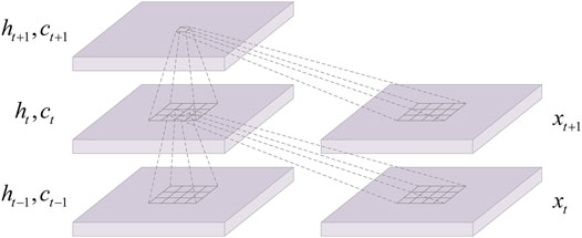
FIGURE 1. Inner structure of ConvLSTM.

2.4 MDN

The MDN can predict PDFs of the target variables, which was first introduced by Christopher M. Bishop in the 1990s. The structure of MDN is composed of a Gaussian mixture model and a feed-forward network. MDN uses Gaussian function as the basic component and superposes a sufficient number of Gaussian functions in a certain proportion to fit the final PDF. Gaussian function enables the MDN to flexibly and accurately represent arbitrary probability distributions (Zhang et al., 2019b). The output variables of model are used to construct final PDFs, which include mean, standard deviation, and proportion of Gaussian distribution. Theoretically, when the mixing coefficients and Gaussian parameters are correctly chosen, MDN can approximate any PDF (Bishop, 1994).

For any given value of a, the Gaussian mixture model provides a general form that approximates any conditional density function $p\left(y_t|a\right)$. The equation is as follows:

$\begin{array}{l}p\left(y_t|a\right)={\displaystyle \sum _{k=1}^K{\pi }_k\left(a,t\right)\phi \left(y_t|{\mu }_k\left(a,t\right),{\nu }_k\left(a,t\right)\right)},\\ \forall t\in \{1,\dots ,T\},\forall k\in \{1,\dots ,K\},\end{array}(6)$

where K is the number of components in the mixture model; ${\pi }_k\left(a,t\right)$, ${\mu }_k\left(a,t\right)$, and ${\nu }_k\left(a,t\right)$ represent mixing coefficient, mean, and standard deviation of the kth component, respectively. It should be noted that the sum of mixing coefficients must be 1, which can be achieved by controlling the output through the softmax function. The softmax function is given by

$\begin{array}{cc}{\displaystyle \sum _{k=1}^K{\pi }_k\left(a,t\right)}=1,& 0\le {\pi }_k\left(a\right)\le 1\end{array},(7)$

${\alpha }_k\left(a,t\right)=\frac{\exp \left({\pi }_k\left(a,t\right)\right)}{{\displaystyle {\sum }_{l=1}^K\exp \left({\pi }_k\left(a,t\right)\right)}}.(8)$

Similarly, to ensure that the variance is greater than or equal to 0, ${\nu }_k\left(a\right)$ can be reformulated as follows:

${\beta }_k\left(a,t\right)=\exp \left({\nu }_k\left(a,t\right)\right).(9)$

In order to control the output value of the MDN model within reasonable bounds, the modified exponential linear unit (ELU) activation function can be used as follows:

$g\left(a\right)=\text{elu}\left(a\right)+1.(10)$

The loss function of standard MDN is maximum likelihood method, which may lead the loss function to NaN value. The reason is that the function approaches infinitesimal as the input value approaches 0. To mitigate the possibility of NaN value, this study employs continuous ranked probability score (CRPS) as the loss function. CRPS is computed as the integral of the square, which avoids infinitesimal or infinite situations.

3 Analysis of Industrial Load Temporal Relevancy and Relevant Factors

3.1 Industrial Load Temporal Relevancy

Industrial load is time series data, so an essential element of it is time. Temporal relevancy is important information that cannot be ignored. In this study, some industrial load data is randomly selected to perform Pearson correlation analysis on the load at adjacent times and the adjacent daily load at the same time. The analysis results are shown in Figure 2. It can be seen that the degree of correlation between loads in both cases tends to weaken with the increase of the time interval, that is, the load temporal relevancy gradually weakens. Therefore, it is important to select historical load data in a suitable time range as the input features of model.

FIGURE 2

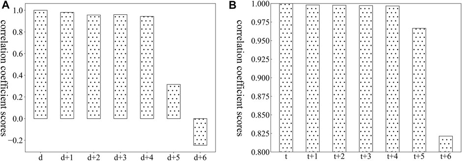
FIGURE 2. Load correlation of adjacent time to d (day) and t (time). (A) shows the Pearson correlation analysis results of adjacent daily loads, and (B) shows the Pearson correlation analysis results of the load at adjacent times.

3.2 Industrial Load Relevant Factors

This study considers two types of relevant factors: temperature and calendar information. First, the influence of temperature on load is analyzed by Pearson correlation coefficient. If the correlation coefficient score is greater than 0.6, temperature is selected as the input feature of the model. Taking the load data of an industrial customer in 2018 as an example, the correlation coefficient score is 0.827, which indicates a strong correlation. Meanwhile, Figure 3 presents the load and temperature profiles. It is obvious that the load increases with decreasing or increasing temperature in winter and summer.

FIGURE 3

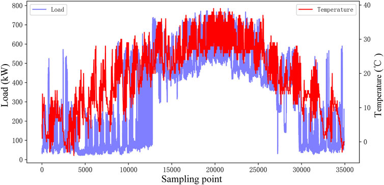
FIGURE 3. Load and temperature profiles.

Calendar information includes working days, weekends and holidays. Industrial loads relate to production plan and activities of workers. Due to the work schedule, the load from Monday to Friday and the load on the weekend are significantly different. In addition, holidays are also an important factor. For example, in China, during important traditional festivals such as the Spring Festival, the National Day, and the Mid-Autumn Festival, employees of most industrial enterprises rest. Therefore, we cannot ignore the effect of calendar information on the load.

4 The Load Forecasting Framework Based on ConvLSTM-MDN Model

This study proposes a deep model for probability density forecasting of industrial load, based on ConvLSTM-MDN. The framework of the proposed method is established by three steps, including data pro-processing, 1D time series to 2D matrices transforming and probability density forecasting of industrial load. Each step in the framework is introduced in the following sections.

4.1 Data Pro-Processing

For load data of industrial customers, the main reasons for missing data include acquisition equipment failures and signal transmission interruption. In order to prevent missing data from destroying the continuity of load data, the following method is adopted: when the proportion of missing data on a certain day is low, linear interpolation is employed to process these data. Instead, all data for the day are deleted.

Then, in order to accelerate convergence speed of the model, we use the min-max normalization (Farsi et al., 2021) method to scale load data and temperature data to the range (0,1). Because the calendar information is discrete data, we adopt One-Hot encoding method to convert it into a form that can be processed by deep learning algorithms. This study marks Monday–Friday as 0 and weekends as 1. According to the actual holiday date of industrial customer, the holiday is marked as 1, and other days are marked as 0.

4.2 1D Time Series to 2D Matrices Transforming

Although the ConvLSTM algorithm takes into account the advantages of the CNN in feature extraction and the LSTM in sequential learning, the use of ConvLSTM in industrial load forecasting will face the problem of data dimension mismatch, that is, the structure of standard ConvLSTM is not suitable for directly processing load data which is 1D time series data. To tackle this problem, we adopted a method to convert the 1D data into 2D matrices that can be processed by ConvLSTM.

The load dataset is denoted as D = {l₁, l₂, …, l_S} with K instances per day; the temperature dataset, date dataset, and holiday dataset are denoted as T = {T₁, T₂, …, T_S}, W = {W₁, W₂, …, W_S}, and H = {H₁, H₂, …, H_S}, respectively. We reconstruct these time series into a series of 2D matrices [N×M], where N is manually set, M is equal to (K+3), and they are integers and greater than 2. The reconstruction method is as follows.

First, construct the first matrix graph: The l₁ to l_K data on the first day are the first row of the matrix. The l_K+1 to l_2K data of the second day are the second row of the matrix. N days of data are selected to construct the 2D matrix [N×K]. Then, temperature, date type, and holiday corresponding to the moment of the first column load are added to the matrix in order to obtain the first 2D matrix [N×M]. This matrix can be used to predict l_N×k+1 data. The first 2D matrix is as follows:

$\{\begin{array}{cccccc}{l}_1& \cdots & l_K& T_1& W_1& H_1\\ ⋮& \ddots & ⋮& ⋮& ⋮& ⋮\\ l_{\left(N-1\right)\times K+1}& \cdots & l_{N\times K}& T_{\left(N-1\right)\times K+1}& W_{\left(N-1\right)\times K+1}& H_{\left(N-1\right)\times K+1}\end{array}\}.(11)$

Second, other matrix graphs are constructed: a fixed-length sliding window method of 1D time series load dataset (with a length of N×K and one step size) is used to capture the other load matrix. That is, the l₂ to l_K+1 data are the first row of the second matrix. The l_K+2 to l_2K+1 data are the second row of the second 2D matrix. N rows of data are selected to construct the second load matrix. The second matrix is also obtained by adding temperature, date type, and holidays to the load matrix in order. The second matrix can be used to predict l_N×K+2 data.

Finally, following the fixed-length sliding window method described before, the last 2D matrix is obtained. A total of (S-N×K) 2D matrices can be obtained. Figure 4 shows the diagram of 2D matrix conversion.

FIGURE 4

FIGURE 4. Diagram of 1D time series to 2D matrix transforming.

4.3 Probability Density Forecasting of Industrial Load

1) Hyper-Parameters Optimization

Hyper-parameters are important factors that directly influence the prediction accuracy of models. In this study, the prediction accuracy is largely related to ConvLSTM layer parameters (number of filters, kernel size) and MDN parameters (the number of components). Too many filters will increase model training time and result in overfitting. On the contrary, models may not get good accuracy results. In addition, a larger kernel size can capture better global features, but the amount of calculation will slow down training process. A smaller kernel size can improve learning speed, but may not capture features well. Similarly, appropriate number of components can better fit PDFs.

Therefore, we applied the grid search method for the hyper-parameter optimization. The grid search method loops through all selectable candidates to find the optimal parameters set. This method is simple to implement and has great versatility. It is described as follows: Given the possible values of three hyper-parameters, then find the optimal set of hyper-parameters that minimizes the validation loss. Table 1 shows the search space of the three hyper-parameters in ConvLSTM layer and MDN. The other benchmark models included in this study use the similar approach to optimize the model hyper-parameters.

2) ConvLSTM-MDN Model

TABLE 1

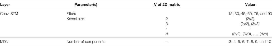
TABLE 1. Hyper-parameters of ConvLSTM layer and MDN.

The converted 2D matrices are used as the input data of the model. The input set is a dimensional tensor with (Y, 1, N, M, 1) size, where Y is the number of samples. The model designed in this study is composed of ConvLSTM layer, flatten layer, dense layer, and MDN. The number of three layers is 1. The activation function of ConvLSTM layer is a rectified linear unit (ReLU). The flatten layer is a transition layer which can flatten the multidimensional array into a linear vector. The dense layer is used to extract the association between the previous features, and the activation function of dense layer is linear function. Afterward, the hidden layers mentioned earlier are merged into MDN to output the approximated parameters (m mean values, m standard deviation, and m mixing coefficients) in parallelized manner, where m is the number of components in the MDN model. The future PDFs are obtained according to the approximated parameters. Furthermore, the loss function of the model is CRPS.

3) Evaluation Metrics

To evaluate the deterministic forecasting performance of the proposed model, two commonly used evaluation metrics are adopted in this work, which are RMSE and MAPE. RMSE can measure the deviation between the forecasted and the actual value. But it is sensitive to data that fluctuates greatly in short time. MAPE measures the accuracy by calculating the relative error between the forecasted value and the actual value, which can solve the problem of RMSE. If the actual value is zero, MAPE cannot be calculated. The advantages of two evaluation metrics can be leveraged. The aforementioned evaluation metrics are defined as follows:

$RMSE=\sqrt{\frac{1}{n}{\displaystyle \sum _{i=1}^n{\left({\widehat{y}}_i-y_i\right)}^2}},(12)$

$MAPE=\frac{100\%}{n}{\displaystyle \sum _{i=1}^n\left|\frac{{\widehat{y}}_i-y_i}{y_i}\right|}.(13)$

Furthermore, we select CRPS as probabilistic evaluation metrics to evaluate the performance of predicted PDF. CRPS is widely used in the field of probabilistic forecasting, which can comprehensively assess the calibration and sharpness of the forecasted PDF. CRPS is expressed as follows:

$CRPS=\frac{1}{n}{\displaystyle \sum _{i=1}^n{\displaystyle \underset{-\infty }{\overset{+\infty }{\int }}{\left[\stackrel{⌢}{F}\left(x\right)-F\left(x\right)\right]}^{2}dx}}.(14)$

The general research framework based on the ConvLSTM-MDN model is visualized in Figure 5.

FIGURE 5

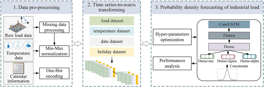
FIGURE 5. Load forecasting framework based on the ConvLSTM-MDN model.

5 Case Study

The proposed model is tested on three different types of industrial customers to assess the feasibility of the probabilistic forecasting method in load forecasting for industrial customers. Two industrial datasets are collected from a nonferrous metal smelting industry and a medical industry in Hunan Province, China, with a temporal resolution is 15-min interval. Another dataset is retrieved from the Irish Smart Metering Electricity Customer Behaviour Trials (CBTs) (Commission for Energy Regulation (CER), 2012). Temperature data are acquired from the National Oceanic and Atmospheric Administration (NOAA) website. After converting the aforementioned data into 2D matrices by using the fixed-length sliding window method mentioned in Subsection 4.2, the input dataset of the model is obtained. Then, 70% of the input dataset is dedicated to training, 10% for validating, and 20% for testing.

For the sake of comparison, eight different models are integrated into the MDN to construct PDFs with the same dataset, including linear regression (LR), autoregressive integrated moving average model (ARIMA), SVR, random forest (RF), feedforward neural network (FFNN), LSTM, 2D-CNN, and 2D-CNN-LSTM. The hyper-parameters of all models are given in Table 2. The first to sixth model in the contrast models directly use 1D time series data as the input data. The rest of model use 2D matrices as input data. The activation function of the neural network in all models is ReLU. Adam Optimizer is used to optimize the network parameters to minimize loss function. The number of components in the MDN network of all contrast models is 3.

TABLE 2

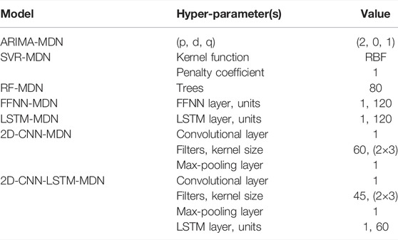
TABLE 2. Hyper-parameters of the contrast models.

5.1 Experiment 1: Load Forecasting of the Nonferrous Metal Smelting Industrial Customer

The nonferrous metal smelting industry data collected between 1 March 2018 and 31 August 2018 are selected for a short-term probability density function forecasting case study. After converting a 1D time series to 2D matrices, the input dataset is split into three parts for training (1 March 2018 to 6 July 2018), validation (7 July 2018 to 24 July 2018), and testing (25 July 2018 to 31 August 2018).

5.1.1 2D Matrix Size Analysis

According to the conversion method described in Subsection 4.2, the size of converted 2D matrix is [N×M]. From Section 3.1, we know that temporal relevancy between loads weakens as the time interval increases. Since the M of the matrix is fixed, time length of historical load is determined by N. Too large N may result in longer processing time and running out of memory. On the contrary, too small N may lead to insufficient extraction of information. Therefore, we need to select an appropriate value of N. Considering the processing time, we set the value range of N to [2,7] in this study. By comparing the optimal result corresponding to each N, the N with minimum error is selected as the final N. The result corresponding to each N is shown in Table 3.

TABLE 3

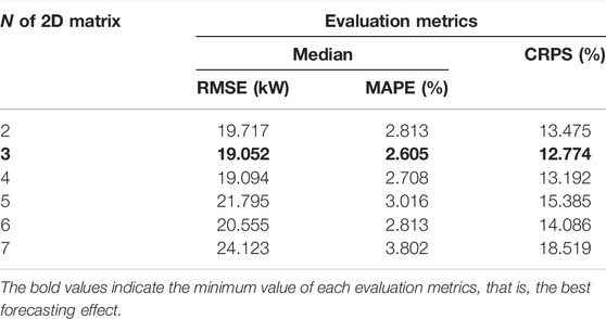
TABLE 3. Forecasting results of each N.

It is observed that the most accurate results are obtained when N = 3, that is, the RMSE, MAPE, and CRPS values are lower than the other values of N. When N = 7, the three error are the largest. The difference between the error of other N is little. Furthermore, the optimal hyper-parameters (filters, kernel size, and the number of components in the MDN) of the model corresponding to N = 3 are 30, (2 × 2), and 3.

5.1.2 Forecasting Result

After determining the size of 2D matrix and hyper-parameters of the model, training set and validation set are used to train the model to obtain the optimal model. Finally, the testing set is input into the optimized ConvLSTM-MDN model to forecast PDFs of industrial load. Figure 6 shows the predicted PDFs for two different times of a day in the testing set and associated real values. Figure 6A,B show the PDFs for peak hours and off-peak hours, respectively. As shown in the figures, real values are very close to the peak of the PDF curve, especially real value in Figure 6B almost coincides with the peak, which indicates that the sharpness of predicted PDF is clear.

FIGURE 6

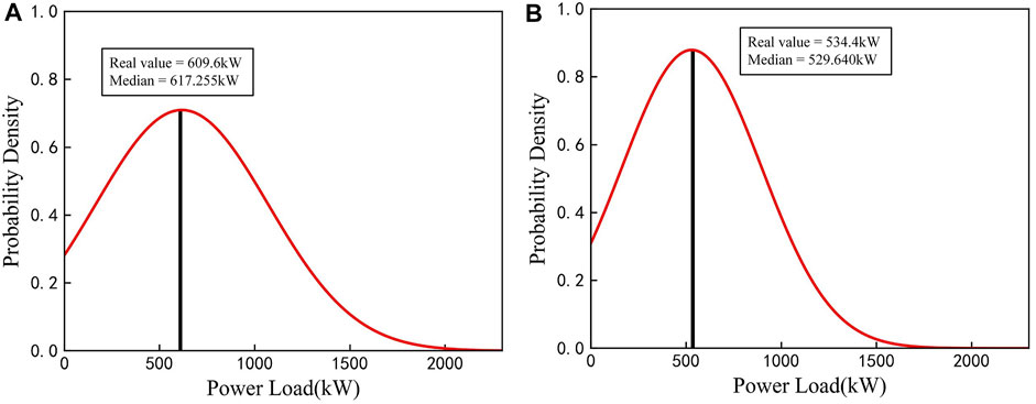
FIGURE 6. ConvLSTM-MDN model predictive distribution and real values for a day at (A) 8:00 and (B) 16:00 in experiment 1.

Taking two sample days in testing set as an example, the PIs under different confidence level obtained by the proposed ConvLSTM-MDN framework are shown in Figure 7. As presented in Figure 7, the PIs under a higher confidence level can cover the PIs under a lower confidence level. In addition, the PIs under different confidence levels and real values of the load have similar fluctuation. Since the PIs under a low confidence level is narrower than the PIs under a high confidence level, the small number of real loads falls outside the PI with lowest confidence level. The PIs becomes narrower when the value of load rises or falls rapidly, and the PIs for peak hours become wider.

FIGURE 7

FIGURE 7. PIs under different confidence levels obtained by the proposed ConvLSTM-MDN model in experiment 1.

5.1.3 Comparisons Analysis

The forecasting result comparisons between the proposed model and contrast models are all provided in Table 4, with the best performance being highlighted. In the table, the forecasting effect of statistical method integrated into the MDN obviously worse than machine learning algorithms integrated into the MDN, and shallow machine learning algorithms worse than deep learning algorithms. For deep learning algorithms, the model combining 2D-CNN and LSTM can achieve better performance than LSTM and 2D-CNN alone for forecasting. The ConvLSTM, which leverages the strengths of CNN and LSTM, performs better than 2D-CNN-LSTM. For instance, the RMSE improvement rates is 19.64%, the MAPE improvement rates is 27.67%, and the CRPS improvement rates is 26.67%. It indicates that ConvLSTM can better capture features of industrial load. In addition, the application of ConvLSTM network to the load forecasting of industrial customers is feasible and effective. Compared with comparison models, the proposed model achieves the most accurate results, which shows the superiority of the model in PLF and DLF. Above all, it can be concluded that the ConvLSTM-MDN model is effective for solving the load forecasting problem of industrial customers.

TABLE 4

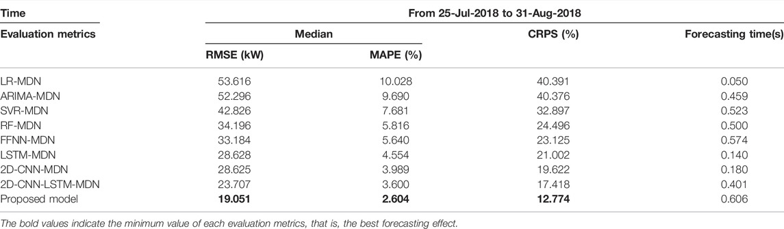
TABLE 4. Load forecasting evaluation on the testing set.

In order to clearly display the prediction results of all models, the load of 2 days in the testing set is selected for further analysis, as shown in Figure 8. It is observed that the load of industrial customer in experiment 1 has strong volatility and high nonlinearity, which brings challenges to all models. According to curves in the figure, contrast models have large deviations from the real load, but the proposed model in this study generally fits and catches the trend of actual load.

FIGURE 8

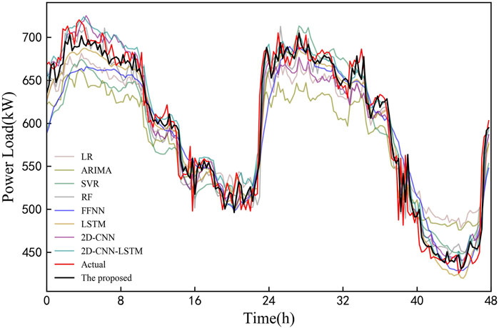
FIGURE 8. Load forecasting profiles of all models in experiment 1.

5.2 Experiment 2: Load Forecasting of Medical Industrial Customer

In this experiment, the load data of the medical industry from 1 March 2018 to 31 August 2018 are used to run simulations. Similarly, the approximate time range of testing set is from 25 July 2018 to 31 August 2018.

5.2.1 2D Matrix Size Analysis

According to the comparison in Table 5, the most accurate results are obtained when N = 4. Although the values of three evaluation metrics fluctuate with the change of N, the fluctuation range is small, that is, the difference between the maximum and minimum of RMSE, MAPE, and CRPS is 1.288, 0.25, and 1.315, respectively. It reflects the stability of the model under different input features. Furthermore, in the case of N = 4, filters, kernel size and the number of components are 75, (2 × 2), and 3.

TABLE 5

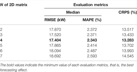
TABLE 5. Forecasting results of each N

5.2.2 Forecasting Result

Figure 9 shows the PDFs of the peak hour (Figure 9A) and off-peak hour (Figure 9B) of a day in the testing set and the associated real values. It can be observed from the figure that real values all falls near the peak of the PDF curve, especially real value in Figure 9B is the closest to the peak. It indicates that the high forecasting accuracy of the proposed model.

FIGURE 9

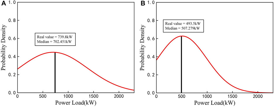
FIGURE 9. ConvLSTM-MDN model predictive distribution and real values for a day at (A) 8:45 and (B) 23:00 in experiment 2.

Figure 10 shows the PIs under different confidence level obtained by the proposed ConvLSTM-MDN model and real values in two sample days. It can be seen that a few real values fall outside the PI with lowest confidence level, and all real values fall within the PI with highest confidence level. The PIs under all confidence levels and real values of the load have similar fluctuation trend, which shows that the proposed model can capture the dynamic changes of the load.

FIGURE 10

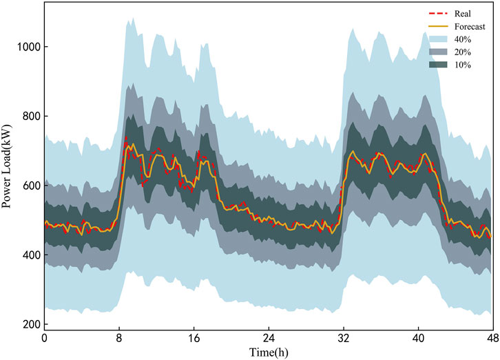
FIGURE 10. PIs under different confidence levels obtained by the proposed ConvLSTM-MDN model in experiment 2.

5.2.3 Comparisons Analysis

Table 6 shows the evaluation metrics of all models on the testing set. The performance of deep learning algorithms integrated into the MDN significantly outperform the performance of shallow machine learning algorithms and statistical method integrated into the MDN in the term of all metrics. Among contrast models, the 2D-CNN-LSTM-MDN model has the best forecasting results. But compared with the 2D-CNN-LSTM-MDN model, the ConvLSTM-MDN model has the minimum errors, which indicate that the proposed model improves the forecasting accuracy. Although the forecasting time is the longest, it is acceptable in practical application with the popularization of cloud computing.

TABLE 6

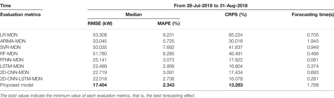
TABLE 6. Load forecasting evaluation on the testing set.

Figure 11 shows the comparison between the prediction results and actual values for 2 days in the testing set. It is observed that the proposed model can better fit the trend of actual load, and other models have large deviations from the real load, especially the LR-MDN model.

FIGURE 11

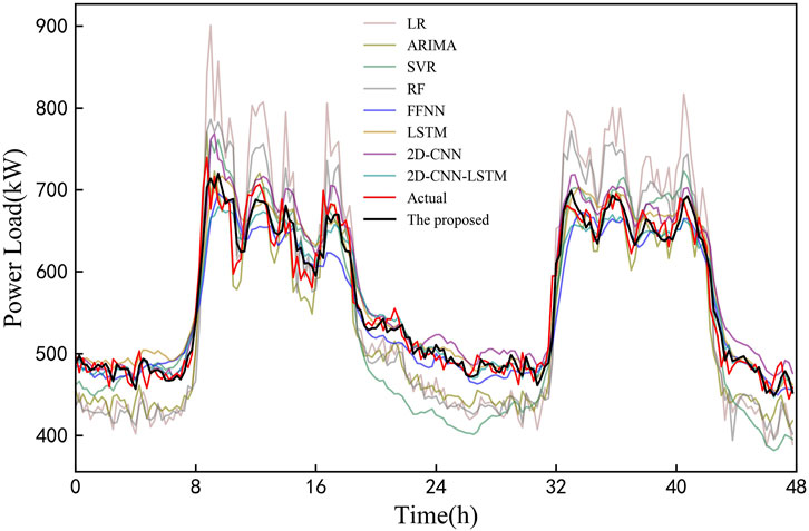
FIGURE 11. Load forecasting profiles of all models in experiment 2.

5.3 Experiment 3: Load Forecasting of the Irish Industrial Customer

In this experiment, public dataset small-to-medium industrial customer collected from Irish is from 1 January 2010 to 31 December 2010 with a 30-min interval. According to the splitting rules, the approximate time range of testing set is from 21 October 2010 to 31 December 2010.

5.3.1 2D Matrix Size Analysis

Table 7 shows the minimum error for each N. This experiment also achieves the best forecasting result when N = 4, which is the same as experiment 2. In the case of N = 4, filters, kernel size and the number of components are 15, (2 × 2), and 3. There is a significant difference between Irish industrial load and other industrial loads, for example, the maximum values of the three industrial loads are 8.257 kWh, 971.2 kWh, and 785.4 kWh. Therefore, the value of the evaluation metrics in this experiment is completely different from the evaluation metrics in the previous two experiments.

TABLE 7

TABLE 7. Forecasting results of each N.

5.3.2 Forecasting Result

Figure 12 shows the PDFs of the peak hour and off-peak hour of a day in the testing set and the associated real values. It can be observed from the figure that the real value in Figure 12A is the closest to the peak. Figure 13 shows the PIs under different confidence level and real values in two sample days. In order to better display the forecasting result, we adjust the value of confidence level. As the value of confidence level decreases, real values that falls outside the PI increases. In addition, The PIs under all confidence levels can capture the dynamic changes of the load.

FIGURE 12

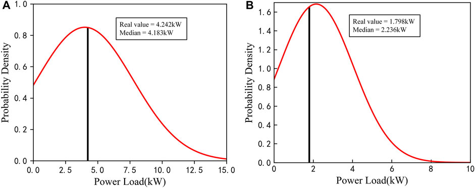
FIGURE 12. ConvLSTM-MDN model predictive distribution and real values for a day at (A) 10:00 and (B) 13:00 in experiment 3.

FIGURE 13

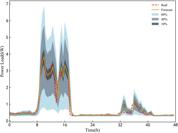
FIGURE 13. PIs under different confidence levels obtained by the proposed ConvLSTM-MDN model in experiment 3.

5.3.3 Comparisons Analysis

Table 8 shows the evaluation metrics of all models on the testing set. The results of shallow machine learning algorithms are far inferior to deep learning algorithms. Among all the models, the proposed model has the best forecasting performance. Figure 14 shows the comparison between the prediction results and actual values for 2 days in the testing set. It can be seen that contrast models are quite different from the real load, and the proposed model can better fit the trend of actual load.

FIGURE 14

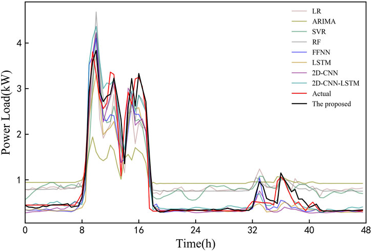
FIGURE 14. Load forecasting profiles of all models in experiment 3.

TABLE 8

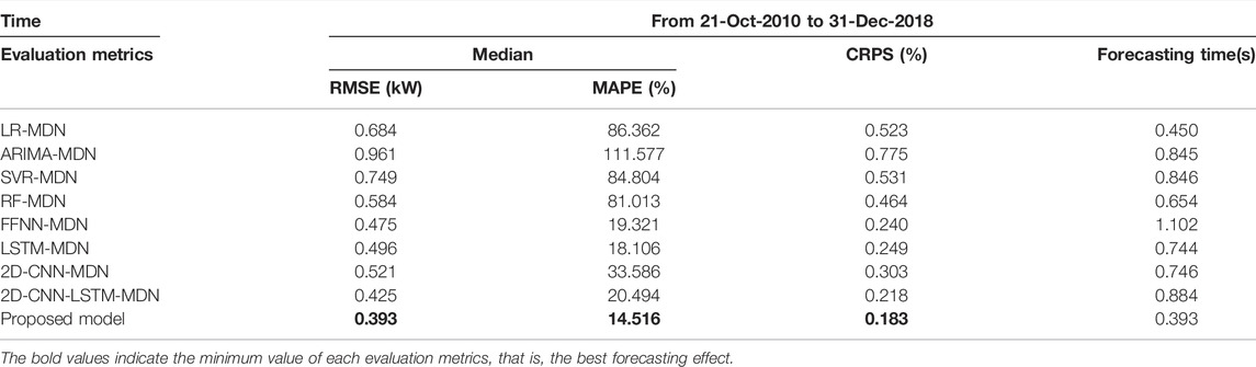
TABLE 8. Load forecasting evaluation on the testing set.

6 Conclusion

In this study, we propose a new probabilistic forecasting method, which can capture the uncertainty of a single industrial customer’s load. By restructuring the load and various relevant factors into 2D matrices using a sliding-window approach, the forecasting model—ConvLSTM-MDN—was applied to the short-term probability forecasting problem of industrial loads. In order to verify the performance of the proposed method, this study builds the classical statistical methods, state-of-the-art deep- and shallow-based models for comparison, and conducts numerical simulations in three experiments. The following results were noted.

1) For three completely different industrial customers, the experimental results of 2D matrix size analysis show that the best forecasting results are obtained when N is 3 or 4. Therefore, when N is in the range of (3, 4), the historical load of a reasonable time interval can be obtained as input feature, which can not only ensure the forecasting accuracy but also reduce the training time.

2) The proposed model takes full advantage of the capabilities of ConvLSTM in feature extraction and sequence learning and the capabilities of MDN in describing uncertainty. The final results show that the model can effectively improve the forecasting accuracy of industrial load. For example, 15–60% improvement in accuracy compared to deep-based models.

3) The hybrid model used in this study is not complex, and a variety of external factors are considered, which is beneficial to be extended to various industrial customers. The forecasting results for three industrial customers show that the model generalizes well.

In our future work, we will study how to reduce computational demand and training time when the value of N increases. Moreover, the feature factors affecting industrial customer such as electricity price will be considered to improve forecasting accuracy.

Data Availability Statement

The data analyzed in this study are subject to the following licenses/restrictions: Because the load data of industrial enterprises are a commercial secret, they cannot be disclose. Requests to access these datasets should be directed to yuanyuan.wang.1980@ieee.org.

Author Contributions

YW: resources, supervision, project administration, and funding acquisition. TW: experiments, research methods, data processing, and write the original draft. XC: guide experiments. XZ: project administration, fund acquisition. JH: perform the writing-review on references. XT: funding acquisition.

Funding

This work is supported by the National Natural Science Foundation of China (No. 52177069), National Natural Science Foundation of China (No. 51777014), Hunan Provincial Key Research and Development Program (No. 2018GK 2057), Research projects funded by Department of Education of Hunan Province of China (18A124), and National Natural Science Foundation of Hunan Provincial (2020JJ5585).

Conflict of Interest

The authors declare that the research was conducted in the absence of any commercial or financial relationships that could be construed as a potential conflict of interest.

Publisher’s Note

All claims expressed in this article are solely those of the authors and do not necessarily represent those of their affiliated organizations, or those of the publisher, the editors, and the reviewers. Any product that may be evaluated in this article, or claim that may be made by its manufacturer, is not guaranteed or endorsed by the publisher.

References

Afrasiabi, M., Mohammadi, M., Rastegar, M., and Afrasiabi, S. (2021). Advanced Deep Learning Approach for Probabilistic Wind Speed Forecasting. IEEE Trans. Ind. Inf. 17 (1), 720–727. doi:10.1109/tii.2020.3004436

CrossRef Full Text | Google Scholar

Afrasiabi, M., Mohammadi, M., Rastegar, M., Stankovic, L., Afrasiabi, S., and Khazaei, M. (2020). Deep-Based Conditional Probability Density Function Forecasting of Residential Loads. IEEE Trans. Smart Grid 11 (4), 3646–3657. doi:10.1109/tsg.2020.2972513

CrossRef Full Text | Google Scholar

Berk, K., Hoffmann, A., and Müller, A. (2018). Probabilistic Forecasting of Industrial Electricity Load with Regime Switching Behavior. Int. J. Forecast. 34 (2), 147–162. doi:10.1016/j.ijforecast.2017.09.006

CrossRef Full Text | Google Scholar

Bishop, C. M. (1994). Mixture Density Networks. Citeseer, Princeton, NJ, USA: Rep. NCRG/94/004.

Google Scholar

Cai, Y., Huang, T., Bompard, E., Cao, Y., and Li, Y. (2017). Self-Sustainable Community of Electricity Prosumers in the Emerging Distribution System. IEEE Trans. Smart Grid 8 (5), 2207–2216. doi:10.1109/tsg.2016.2518241

CrossRef Full Text | Google Scholar

Cai, Y., Liu, Y., Tang, X., Tan, Y., and Cao, Y. (2021). Increasing Renewable Energy Consumption Coordination with the Monthly Interprovincial Transaction Market. Front. Energ. Res. 9, 719419. doi:10.3389/FENRG.2021.719419

CrossRef Full Text | Google Scholar

Commission for Energy Regulation (Cer) (2012). CER Smart Metering Project Electricity Customer Behaviour Trial. [Online]. Available at: https://www.ucd.ie/issda.

Google Scholar

Da Silva, F. L. C., Cyrino Oliveira, F. L., and Souza, R. C. (2019). A Bottom-Up Bayesian Extension for Long Term Electricity Consumption Forecasting. Energy 167, 198–210. doi:10.1016/j.energy.2018.10.201

CrossRef Full Text | Google Scholar

Essien, A., and Giannetti, C. (2020). A Deep Learning Model for Smart Manufacturing Using Convolutional LSTM Neural Network Autoencoders. IEEE Trans. Ind. Inf. 16 (9), 6069–6078. doi:10.1109/tii.2020.2967556

CrossRef Full Text | Google Scholar

Fallah, S. N., Ganjkhani, M., Shamshirband, S., and Chau, K. W. (2019). Computational Intelligence on Short-Term Load Forecasting. A Methodological Overview” 12 (3). doi:10.3390/en12030393

CrossRef Full Text | Google Scholar

Farsi, B., Amayri, M., Bouguila, N., and Eicker, U. (2021). On Short-Term Load Forecasting Using Machine Learning Techniques and a Novel Parallel Deep LSTM-CNN Approach. IEEE Access 9, 31191–31212. doi:10.1109/access.2021.3060290

CrossRef Full Text | Google Scholar

He, Y., Liu, R., Li, H., Wang, S., and Lu, X. (2017). Short-term Power Load Probability Density Forecasting Method Using Kernel-Based Support Vector Quantile Regression and Copula Theory. Appl. Energ. 185, 254–266. doi:10.1016/j.apenergy.2016.10.079

CrossRef Full Text | Google Scholar

He, Y., Qin, Y., Wang, S., Wang, X., and Wang, C. (2019). Electricity Consumption Probability Density Forecasting Method Based on LASSO-Quantile Regression Neural Network. Appl. Energ. 233-234, 565–575. doi:10.1016/j.apenergy.2018.10.061

CrossRef Full Text | Google Scholar

Hong, Y.-Y., Martinez, J. J. F., and Fajardo, A. C. (2020). Day-Ahead Solar Irradiation Forecasting Utilizing Gramian Angular Field and Convolutional Long Short-Term Memory. IEEE Access 8, 18741–18753. doi:10.1109/access.2020.2967900

CrossRef Full Text | Google Scholar

Hou, H., Liu, P., and Xiao, Z. f. (2021). Capacity Configuration Optimization of Standalone Multi-Energy Hub Considering Electricity, Heat and Hydrogen Uncertainty. IET Energ. Convers. Econ. 2021, 12028. doi:10.1049/enc2.12028

CrossRef Full Text | Google Scholar

Hou, H., Xu, T., and Wu, X. X. (2020). Optimal Capacity Configuration of the Wind-Photovoltaic-Storage Hybrid Power System Based on Gravity Energy Storage System. Appl. Energ. 271, 115052. doi:10.1016/j.apenergy.2020.115052

CrossRef Full Text | Google Scholar

Hou, H., Xue, M. Y., and Xu, Y. (2020). Multi-objective Economic Dispatch of a Microgrid Considering Electric Vehicle and Transferable Load. Appl. Energ. 262, 114489. doi:10.1016/j.apenergy.2020.114489

CrossRef Full Text | Google Scholar

Jiao, R., Zhang, T., Jiang, Y., and He, H. (2018). Short-Term Non-residential Load Forecasting Based on Multiple Sequences LSTM Recurrent Neural Network. IEEE Access 6, 59438–59448. doi:10.1109/access.2018.2873712

CrossRef Full Text | Google Scholar

Kuster, C., Rezgui, Y., and Mourshed, M. (2017). Electrical Load Forecasting Models: A Critical Systematic Review. Sustain. Cities Soc. 35, 257–270. doi:10.1016/j.scs.2017.08.009

CrossRef Full Text | Google Scholar

López, J. C., Rider, M. J., and Wu, Q. (2019). Parsimonious Short-Term Load Forecasting for Optimal Operation Planning of Electrical Distribution Systems. IEEE Trans. Power Syst. 34 (2), 1427–1437.

Google Scholar

National Bureau of Statistics of the People’s Republic of China (2021). China Energy Statistical Yearbook 2020. Beijing, China: China Statistics Press, 195–199.

Google Scholar

Ruan, Y. J., Wang, G., Meng, H., and Qian, F. Y. (2021). A Hybrid Model for Power Consumption Forecasting Using VMD-Based the Long Short-Term Memory Neural Network. Front. Energ. Res. 9.

Google Scholar

Shi, X., Chen, Z., and Wang, H. (2015). Convolutional LSTM Network: A Machine Learning Approach for Precipitation Nowcasting. Proc. 28th Int. Conf. Neural Inf. Process. Syst. 2015, 802–810.

Google Scholar

Sun, Z., and Zhao, M. (2020). Short-Term Wind Power Forecasting Based on VMD Decomposition, ConvLSTM Networks and Error Analysis. IEEE Access 8, 134422–134434. doi:10.1109/access.2020.3011060

CrossRef Full Text | Google Scholar

Tan, M., Yuan, S., Li, S., Su, Y., Li, H., and He, F. H. (2020). Ultra-Short-Term Industrial Power Demand Forecasting Using LSTM Based Hybrid Ensemble Learning. IEEE Trans. Power Syst. 35 (4), 2937–2948. doi:10.1109/tpwrs.2019.2963109

CrossRef Full Text | Google Scholar

Wang, R., Xia, X. Y., Li, Y. P., and Cao, W. M. (2021). Clifford Fuzzy Support Vector Machine for Regression and its Application in Electric Load Forecasting of Energy System. Front. Energ. Res. 9. doi:10.3389/fenrg.2021.793078

CrossRef Full Text | Google Scholar

Wang, Y., Chen, J., Chen, X., Zeng, X., Kong, Y., Sun, S., et al. (2021). Short-Term Load Forecasting for Industrial Customers Based on TCN-LightGBM. IEEE Trans. Power Syst. 36 (3), 1984–1997. doi:10.1109/tpwrs.2020.3028133

CrossRef Full Text | Google Scholar

Wang, Y., Kong, Y., Tang, X., Chen, X., Xu, Y., Chen, J., et al. (2020). Short-Term Industrial Load Forecasting Based on Ensemble Hidden Markov Model. IEEE Access 8, 160858–160870. doi:10.1109/access.2020.3020799

CrossRef Full Text | Google Scholar

Wang, Y., Sun, S., Chen, X., Zeng, X., Kong, Y., Chen, J., et al. (2021). Short-term Load Forecasting of Industrial Customers Based on SVMD and XGBoost. Int. J. Electr. Power Energ. Syst. 129, 106830. doi:10.1016/j.ijepes.2021.106830

CrossRef Full Text | Google Scholar

Xie, W., Zhang, P., Chen, R., and Zhou, Z. (2019). A Nonparametric Bayesian Framework for Short-Term Wind Power Probabilistic Forecast. IEEE Trans. Power Syst. 34 (1), 371–379. doi:10.1109/tpwrs.2018.2858265

CrossRef Full Text | Google Scholar

Zhang, H., Liu, Y., Yan, J., Han, S., Li, L., and Long, Q. (2020). Improved Deep Mixture Density Network for Regional Wind Power Probabilistic Forecasting. IEEE Trans. Power Syst. 35 (4), 2549–2560. doi:10.1109/tpwrs.2020.2971607

CrossRef Full Text | Google Scholar

Zhang, J., Yan, J., Infield, D., Liu, Y., and Lien, F.-s. (2019). Short-term Forecasting and Uncertainty Analysis of Wind Turbine Power Based on Long Short-Term Memory Network and Gaussian Mixture Model. Appl. Energ. 241, 229–244. doi:10.1016/j.apenergy.2019.03.044

CrossRef Full Text | Google Scholar

Zhang, W., Quan, H., and Srinivasan, D. (2019). An Improved Quantile Regression Neural Network for Probabilistic Load Forecasting. IEEE Trans. Smart Grid 10 (4), 4425–4434. doi:10.1109/tsg.2018.2859749

CrossRef Full Text | Google Scholar

Zhao, X., and Li, R. (2021). A Novel Decomposition and Combination Technique for Forecasting Monthly Electricity Consumption. Front. Energ. Res. 9.

Google Scholar