 Yating Hu1†
 Qiong Zhang
- 1University of Electronic Science and Technology of China, Chengdu, China
- 2Research Institute of Petroleum Exploration and Development, Beijing, China
Due to the complexity of unconventional reservoir measurement, log data acquired are often incomplete, which results in inaccurate formation evaluation and higher operational risks. Common solutions, such as coring, are typically high cost related while not being sufficiently representative. In recent years, neural network has received increasing attention given its strong ability in data prediction. Nevertheless, most neural networks only focus on one specific feature of the selected data, thus prohibiting their prediction accuracy for reservoir logs where data are often dominated by more than one key feature. To address this challenge, a novel multi-channel hybrid Long Short-Term Memory (LSTM) neural network for effective acoustic log prediction is proposed. The network combines Convolutional Neural Network (CNN) and LSTM, where CNN is used to extract spatial features of the logs and LSTM network extracts temporal features with the assistance of an adaptive attention mechanism implemented for key feature recognition. In addition, the strong heterogeneity of unconventional reservoirs also increases the difficulty of prediction. Therefore, according to the characteristics of the unconventional reservoir, we designed three feature enhancement methods to mine the hidden information of logs. To prove the performance of the proposed network, a case study is presented with data acquired from Jimusar Oilfield, one of the largest unconventional reservoirs in China. Four groups of experiments are conducted, and the proposed network is employed for acoustic log prediction. The predicted results are validated against measurement (R2: 92.27%, 91.42%, 93.31%, and 92.03%; RMSE: 3.32%, 3.92%, 3.06%, and 3.53%). The performance of the proposed network is compared to other networks such as CNN, LSTM, CNN-LSTM, and random forest (RF). The comparisons show that the proposed network has the highest accuracy level of prediction, which means it provides an effective approach to complement missing data during complicated unconventional reservoir measurement and, therefore, could be of significant potential in energy exploration.
1 Introduction
As the difficulty of discovering conventional reservoirs increases year by year, the proportion of unconventional reservoirs in the field of oil and gas exploration is increasing. Different from conventional reservoir evaluation, unconventional shale reservoirs must be stimulated by fracturing to obtain industrial hydrocarbon flow (Guo et al., 2019; Wang H. et al., 2016). The key rock mechanical parameters of fracturing can only be obtained through core analysis and acoustic logs (Eshkalak et al., 2014). However, since core experiments are expensive and time consuming, acoustic logs are often used to calculate rock mechanical parameters, such as Poisson’s ratio and Young’s modulus. However, the scale and quality of the data, especially for shear wave slowness (DTS), can be easily affected owing to the complex borehole environment during the operation on site, which results in an even more expensive cost of obtaining the reliable DTS logging in contrast to the compressional wave slowness (DTC).Therefore, the prediction of DTS has been proposed instead of measurement for saving the cost, which has drawn interest from both academic and industrial realms during the last 40 years.
To address this problem, many researchers have tried methods of generating logs. For example, according to parameters such as geological parameters, logs are inverted based on physical models, or logs are obtained by fitting empirical formulas according to other information of logs. Although these methods are very convenient and efficient, the established physical models often greatly simplify the real information of the formation, and the empirical formulas need to be fitted separately for different situations (Castagna et al., 1985; Greenberg & Castagna, 1992). For these reasons, the quality of logs obtained by these two methods cannot be guaranteed.
In recent years, machine learning (ML) has become the mainstream method for well logs prediction because of its advantages of automatically mining the internal relationship of data. Zhang et al. (2018) established a log reconstruction method based on LSTM for acoustic log prediction. Based on assembly of clustering, classification, and regression, Du et al. (2019) proposed a new method to improve the accuracy of shear wave estimation. Feng et al. (2021) used random forest to predict well logs and evaluated simultaneously the uncertainty of the prediction. You et al. (2021) proposed to use transfer learning to improve the performance of LSTM and applied the prediction results to morphology identification and saturation inversion of gas hydrate. Wang et al. (2021) proposed a spatial-temporal neural network (STNN) algorithm that combines the advantages of CNN and LSTM. Also, it successfully predicted acoustic logs from natural gamma, density, compensated neutron, resistivity, and borehole diameter logs. Given the interdependence of the well logs in the depth domain sample sequence, Shan et al. (2021) proposed a new intelligent construction method based on the bi-directional LSTM and CNN. Zhang et al. (2022) used a 1D-CNN to achieve the prediction of DTS for carbonate and sandstone reservoirs, demonstrating that the network outperforms traditional backpropagation neural network (BP) and support vector regression (SVR). Wang et al. (2022) developed a hybrid model of CNN and LSTM to predict shear wave velocity. Zeng et al. (2022) proposed a multi-stage attention mechanism based on the GRU neural network, which realized the prediction of DTC. Pan et al. (2022) demonstrated that the XGBoost algorithm can achieve log prediction by using the grid search method and the genetic algorithm to optimize the hyperparameters. However, most of these studies only consider one single feature, e.g., the temporal or spatial feature of well logs (Pham & Naeini, 2019; Song et al., 2021). Very few of the studies take into account multiple features, nor have fully explored the implicit information between various features. Since many log data are dominated by more than one feature, this leaves room for prediction accuracy enhancement (Zhou et al., 2021). For example, during the reservoir appraisal stage, formation heterogeneity casts a significant impact on prediction accuracy for various logs.
In view of this, this study further investigates the effect of each feature of well logs on the prediction accuracy and develops a neural network for predicting logs of the unconventional reservoir to reduce the cost of hydrocarbon exploration. This study proposes a multi-channel Hybrid Feature Enhancement Network (HFEN) based on CNN-LSTM in the scope of acoustic log prediction, and the log feature enhancement method is investigated to enhance fluctuation trends and expand feature space. The new log feature enhancement method and the extract of each feature by the hybrid network contribute to the improvement of prediction accuracy. The proposed HFEN is validated on field data from Jimusar Oilfield, and satisfactory results are achieved.
2 Workflow of the Proposed Network
2.1 Development Strategy
The sedimentation of the stratum is gradual in time, and the logs have different responses to the sedimentary characteristics of different strata. Therefore, the well log is the ordered sequence along with the depth. LSTM is suitable for predicting data with time-series features, such as well logs (Zhang et al., 2018; Li et al., 2019). However, LSTM only considers the trend of log changes with depth, and the perception of local features is still lacking. The CNN network uses the convolution kernel to capture the local correlation features in the logs, but due to the limitation of the filter size, it is difficult for the network to learn the pre- and post-dependency of the sequence logs (Shan et al., 2021). Therefore, to combine the advantages of the two networks, a parallel structure of CNN and LSTM is proposed in this study, and an attention mechanism is added to the network. The novel multi-channel hybrid feature enhancement network (HFEN) structure is shown in Figure 1.

FIGURE 1. Conceptual overview of the multi-channel CNN-LSTM network.
Existing literature studies have confirmed that introducing domain knowledge can effectively improve the prediction accuracy of neural networks (Chen & Zhang et al., 2018; Downton et al., 2020). Therefore, based on the characteristics of well logs, domain knowledge is introduced into HFEN. Three log feature enhancement methods are designed, which make it easier for the network to learn the feature of log and improve the prediction accuracy. In addition, in the training process, each input feature is treated equally by the neural network, which means that their contribution to the output is the same. However, in fact, different input features have different correlations and similarities with the output, so the attention mechanism is introduced into the network to adjust the importance of each feature. (Wang Y. et al., 2016; Li et al., 2020; Wang et al., 2020). The workflow of the proposed method is shown in Figure 2.
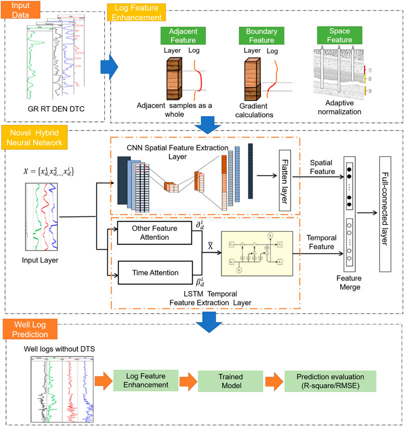
FIGURE 2. Workflow for acoustic prediction using the proposed hybrid feature enhancement network.
In this study, the feature of the log is referred to using three terms. “Log Feature” is used to represent the fluctuating feature of the logs derived from the domain knowledge. “Spatial Feature” represents the spatial feature that exists between logs measuring different physical properties. “Temporal Feature” represents the temporal (depth) continuity of the log. For the attention mechanism, “Other Feature Attention” refers to the importance of logs with different physical properties, and “Time Attention” refers to the importance of different log depths converted to time scale.
2.2 Log Feature Enhancement
The current ML or neural network research focuses on using high-quality data to obtain highly accurate predictions. However, due to the strong heterogeneity in unconventional petroleum resources, the feature mapping relationship between known logs and missing logs is complex and fuzzy, which will reduce the reliability of prediction logs. In addition, in the case of a small input sample size, feature enhancement methods improve the diversity of the sample by emphasizing its feature space and thus compensate small sample size. In this regard, feature enhancement methods guided by domain knowledge are proposed. The three most representative features (adjacent feature, boundary feature, and space feature) of the log are enhanced to strengthen the correlation between the input logs and the output log and to highlight the details of the log.
Based on the logging principle, in the vertical direction, there is a correlation between the log value of the reservoir at a certain point and the log from the adjacent formation (Li et al., 2019), as shown in Figure 3. Therefore, multiple adjacent depth samples are combined as the one input of the network, to realize the adjacent feature enhancement, instead of using conventional single-point-to-single-point prediction. In this study, the upper and lower four points of the sampling point are combined as one sample of input (i.e. five sample points as a whole).
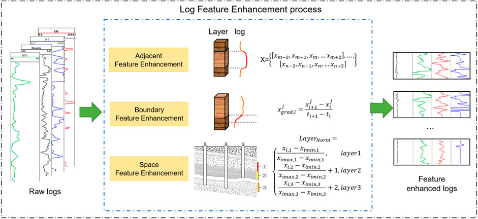
FIGURE 3. The log feature enhancement process includes adjacent feature enhancement, boundary feature enhancement, and space feature enhancement.
For heterogeneous reservoirs, the vertical variation of formation physical properties is large, especially between strata with different properties and types, as shown in Figure 3. Consequently, they change drastically in different small ranges (different small geological layers). However, the log is averaged by the logging tool, which may weaken the reflection of a boundary change, resulting in the correct characteristics that cannot be shown in the target prediction log. Boundary feature enhancement refers to the gradient calculation of the original data in order to make the input data more clearly reflect the vertical changes in the physical properties of the reservoir (Hall et al., 2017). The gradient attribute calculation formula is as follows:
where x is the value of the log samples, m denotes the different logs feature, and n refers to the number of log samples.
The target sweet spot usually contains multiple geological layers as shown in Figure 4. There is some variance in the logs reflecting the characteristics of each geological formation. Intuitively, the distribution of log values is different. If the data of different strata are mapped to the overall stratigraphic interval according to the traditional normalization method, the accuracy of the neural network will be limited (Zhang et al., 2018). Therefore, space feature enhancement is used to solve this problem, that is, different formation layer spaces will be mapped to different numerical ranges for adaptive normalization, which is calculated by Eq. 2. It is worth noting that this enhancement method can be omitted if there is no geological layer depth in some cases.
where
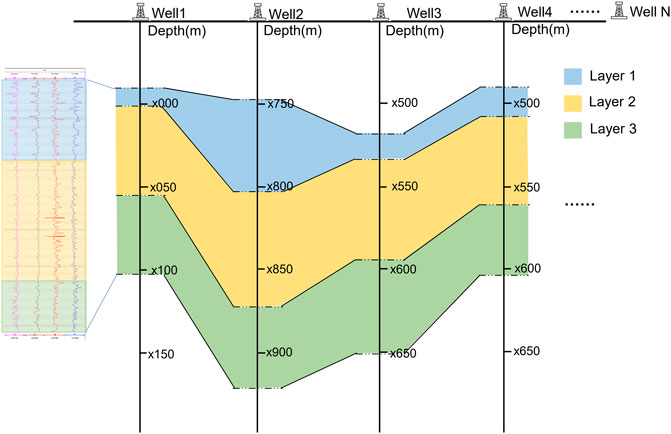
FIGURE 4. Schematic diagram of target formation depth for different wells, which is the known information in the research field.
2.3 Spatial Feature Extraction
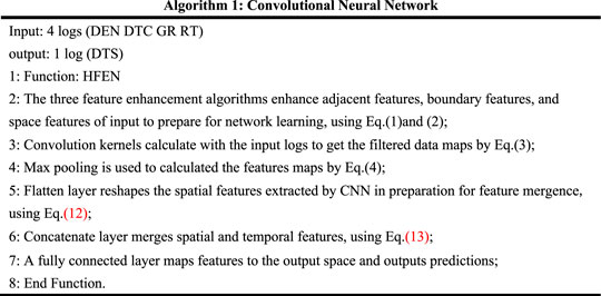
CNN is a feed-forward neural network. Existing studies have shown that the CNN network not only has good performance in image processing, it also has good performance in natural language processing (Yang et al., 2016; Kim et al., 2019). In this study, since the log is typical one-dimensional data, the convolution kernel can only scan along depth dimension, therefore, 1D-CNN is adopted. It consists of three layers: an input layer that accepts raw data, a hidden layer that extracts characteristics, and an output layer. Generally, the hidden layer includes a convolutional and pooling layer, which realize spatial feature extraction and dimensionality reduction, respectively. Convolution calculation and pooling operation are shown in the following equations:
where ∗ is convolution operation;
The algorithm flow of the CNN branch of the hybrid feature enhancement network is as follows.
2.4 Temporal Feature Extraction
2.4.1 Attention Mechanism Implementation
The attention mechanism was first proposed in the field of human vision research (Wang Y. et al., 2016; Lin et al., 2019). In recent years, it has been widely used in engineering applications, such as restoring the missing sensor response and leak detection in the oil pipeline network (Hu et al., 2020; Hu et al., 2021). The attention mechanism allows the network to capture more important ones from different log features. Its specific implementation method is to automatically extract the key information of each feature through calculation and then assign weights according to the similarity between the input log and the target log. The larger the weight, the more important the input log is for predicting the target log. The main role of the attention mechanism introduced into the network is to improve its ability to capture the dynamic features of the data and its interpretability. For this study, the attention mechanism is added to the features dimension and the time dimension, respectively, and finally, their outputs are merged as the input vector of LSTM. The following is a detailed description of them.
Logs acquired at the same depth may have different importance to the predicted log, which is based on the physical quantities they measure, and the principle of measurement. Although, the researcher can judge and choose which logs are more suitable as input according to the previous rules. But in neural networks, it is more inclined to be selected by the network, because it can understand some associations that we cannot intuitively observe. Typically, the network treats any input features equally. Therefore, it is necessary to assign higher weights to logs of greater importance. The method achieved is to introduce the key feature attention mechanism into the network, that is, measure the correlation between the input logs and the target log at the same depth, and extract the most critical feature information for the output.
The logging sequence data can be represented as a matrix X as shown in Eq. 5. The superscript of X represents different logs, such as DEN, DTC, GR, etc., and the subscript represents the depth value corresponding to the sample. For simplicity, it is written in vector
where
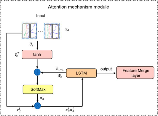
FIGURE 5. The structure of key features attention mechanism module, where
Then, the SoftMax function is used to normalize the score
The introduction of the time attention mechanism can give the relationship between the current moment and other times, and automatically select the key information at different times, avoiding the loss of information in LSTM due to the long input sequence. The attention mechanism strengthens the contribution of important information by assigning different weights to features at different times, making it easier for the network to capture long-distance interdependent features in the sequence. Its structure is the same as that in Figure 5, only the parameters are changed.
where
The time weight,
where
Then, the input of the LSTM network can be obtained from the following equation:
Figure 6 shows the update of the input features importance by the attention mechanism. Figure 6A shows the default importance assigned by the network to each input feature when the attention mechanism is not introduced. Figure 6B shows that the importance of each input feature is automatically updated after the attention mechanism. The importance of DTC is the strongest in prediction, which can also be explained at the physical level because DTC and DTS are both acoustic logs and they have great similarities.
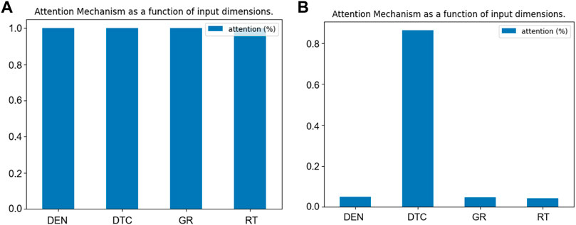
FIGURE 6. (A) The importance of each feature by default. (B) The importance of each feature after the attention mechanism algorithm.
2.4.2 Temporal Feature Extraction
Traditional neural networks have high accuracy in dealing with complex relational mappings, such as CNN and BP, but they cannot effectively deal with historical dependencies of data. To address this problem, recurrent neural networks (RNN) are proposed, which can process dependencies using information accumulated in previous time steps, thereby improving prediction accuracy. But RNN can only handle short-term dependencies, otherwise, there will be a gradient explosion problem. Therefore, LSTM, a recurrent neural network improved by RNN, is proposed. It is a kind of recurrent neural network proposed by Hochreiter & Schmidhuber (1997). LSTM contains a special gate structure (input gate, output gate, and forget gate), which enables a powerful memory function (Mosavi et al., 2019; Ardabili et al., 2022). It has been widely applied in the text analysis, sentiment analysis, speech recognition, and other fields (Long et al., 2019; Rehman et al., 2019; Xie et al., 2019). The log is the typical sequential data, so it is suitable to use LSTM to predict it. Eq. 11 represents the gate mechanism information related to the LSTM network.
where
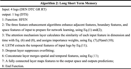
The algorithm flow of the LSTM branch of the hybrid feature enhancement network is as follows:
2.5 Feature Merge Process
For different networks, pertaining feature extraction methods could vary considerably, therefore, it is important to deploy proper methods to enhance prediction accuracy (Li et al., 2019). In HFEN, the CNN branch extracts the spatial feature of sequence data, while the LSTM branch extracts the temporal feature. The two features are consequently merged as input for the fully connected layer, the output of which is the predicted log. Figure 7 shows the complete process of feature merge. As shown in the following, the data acquired from the CNN branch is processed via matrix transformation as shown in Eq. 12, this is to ensure initial data out of CNN and LSTM are of the same dimension for sequential processing, which is commonly referred to as data merging, as shown in Eq. 13. In this step, a concatenate layer is employed. Then, the merged features are mapped to the output space through the fully connected layer, and the output is obtained, in this case, predicted logs.
where Matrix
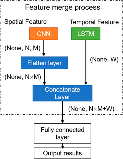
FIGURE 7. Feature merge process.
3 Network Feasibility Validation Using Field Data
3.1 Field Background and Dataset Introduction
The data are collected from the Jimusar Shale Oilfield (referred to as JSO). The Jimusar Shale Oilfield in the Junggar Basin, West China, is an important unconventional oilfield and typical shale oil reservoir that covers a surface area exceeding 300,000 acres, as shown in Figure 8. (Guo et al., 2019). Abundant shale oil was discovered in the Permian Lucaogou Formation. The Lucaogou Formation has the characteristics of large burial depth, poor physical properties, strong heterogeneity, and high crude oil viscosity, and the reservoir lithology is complex and changes rapidly vertically. This results in highly nonlinear relations between logs reflecting different geophysical properties. Due to oilfield environmental factors and cost factors, there is a situation in which the log is missing in the measurement. The method proposed in this study can complement the missing log, which is of great significance for the reservoir analysis, production operations, and even cost reduction.

FIGURE 8. (A) Location of Junggar Basin and (B) location of wells.
Figure 9 shows the relevant data and schemes used in the experiment. The existing logs from four wells are applied to conduct experiments. These logs include density (DEN), natural gamma (GR), deep resistivity (RT), compressional wave slowness data (DTC), and shear wave slowness (DTS), with a sampling interval of 0.125 m. DEN, GR, DTC, and RT are used as input for the prediction of DTS.
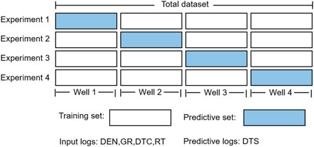
FIGURE 9. Experimental datasets and schemes for predicting DTS.
3.2 HFEN Utilization and Parameter Setup
The HFEN network is utilized to predict DTS based on aforementioned data . The structure of the HFEN is presented in Figure 10 for the given scenario. The network includes a CNN branch and an LSTM branch. In order to identify relevant network parameters, it is critical to search for the optimized balance between accuracy and efficiency. Table 1 shows the finalized parameters for the designated network. The CNN branch contains two CNN layers with a kernel size of three and a max pooling layer with a size of 2. In the LSTM branch, there are two LSTM layers with units of 128 and 64, and two Dropout layers. Finally, the dimension of the output layer is set to 1, since the predicted results are one-dimensional data.
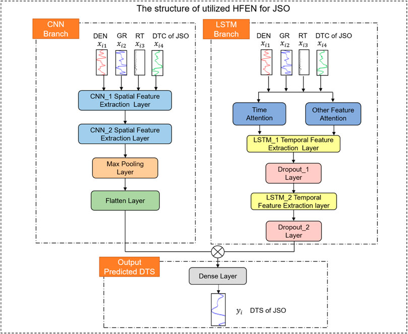
FIGURE 10. The structure of utilized HFEN for JSO.
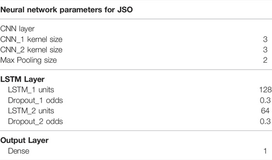
TABLE 1. Neural network parameters.
3.3 Performance Evaluation Indicators
Root mean square error (RMSE) and coefficient of determination (R2) are selected as evaluation indicators in this study, as shown in Eq.14 and 15. The R2 reflects the proximity of the real values and the predicted results. The smaller RMSE, the smaller the deviation between the predicted value and the real value.
where SST is the sum of squares of the difference between the original data and the mean; SSE is the sum of squares of the errors between the fitted data and the corresponding points of the original data.
where
3.4 Performance Evaluation of Hybrid Neural Network
To verify the performance of HFEN, the leave-one-out method is used to conduct experiments, namely the experimental method in Figure 9. The comparison of HFEN with measurement is shown in Table 2. Specifically, in the four experiments, the RMSE of the HFEN prediction compared to the measurement are 3.32%, 3.92%, 3.06%, 3.53%, and the R2 are 92.27%, 91.42%, 93.31%, 92.03%, respectively. Figures 11–14 show the actual measurements of DTS and the predicted DTS via the HFEN network. The black and purple lines represent the actual measurements and prediction of HFEN, respectively. It can be observed from Figures 11–14 that the proposed HFEN achieve a good fitting between the predicted and the measurements. Even though the reservoir in the study area is highly heterogeneous and the geological conditions are complex, the trend of the prediction still matches the trend of the measured data, which shows the advantage of the HFEN network.
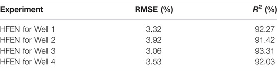
TABLE 2. Comparison of HFEN-predicted results to measurement.

FIGURE 11. HFEN vs. Measurement in well 1.
The prediction results are compared to a few common machine learning algorithms (CNN and LSTM) to verify the ability of HFEN to capture the temporal and spatial features of the logs. The comparison results are shown in Figures 15, 16 and Table 3. The results show that compared to stand-alone CNN and LSTM networks, the prediction results of HFEN have improved significantly. The comparison is made with the base CNN-LSTM network (under the same experimental conditions, except that the feature enhancement methods are not used) to verify the effectiveness of the feature enhancement methods in HFEN. The comparison results are shown in Figures 11–14. The green line in the figure represents the prediction results of base CNN-LSTM. The results demonstrate that compared to the base CNN-LSTM network, the RMSE is reduced by 2.27%, 2.87%, 2.48%, and 2.83%, and the R2 is improved by 6.47%, 6.67%, 7.93%, and 6.05%. It is also compared with the popular integration algorithm, random forest (Breiman, 2001), to verify the performance of HFEN. The results show that the prediction accuracy of HFEN is higher than that of random forest. In addition, the prediction results of the proposed method also show advantages compared with similar studies (Wang and Peng, 2019; Wang et al., 2021; Mehrad et al., 2022). Compared to a previous study regarding the JSO field (Song, et al., 2021), HFEN provides results that are closer to actual measurements with lower errors which prove that the network is effective.

TABLE 3. Comparison of HFEN-predicted results with other methods.
The comparison between base CNN-LSTM and HFEN is used as an example to further analyze the performance of HFEN. In general, the results of both HFEN and base CNN-LSTM reflect the trend of the measured values, as shown in Figures 11–14. However, in terms of numerical accuracy, the novel HFEN is significantly better than the CNN-LSTM model (especially as shown in Figures 12, 14). From 4010 to 4015 m in Figure 11 and 3490–3525 m in Figure 14, the prediction of the base CNN-LSTM model has a large deviation from the actual measurement log, while the predicted result of HFEN is similar to the actual measurement log. The characteristics of the logs of these two experiments are that the logs change greatly due to the influence of formation heterogeneity and the presence of hydrocarbon. The reason for the good performance of HFEN is that the multi-channel hybrid network effectively extracts the spatial and temporal features of logs, fully coupling the features in the logs of different physical measurement principles. In addition, the feature enhancement method extends the feature space of the logs so that the input logs contain more features, and enhances the correlation between the input logs and the target logs, making the network more capable of handling mutation points and the prediction results closer to the actual measurement. This proves that HFEN can accurately predict log trends and values for engineering demand.
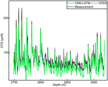
FIGURE 12. HFEN vs. Measurement in well 2.

FIGURE 13. HFEN vs. Measurement in well 3.
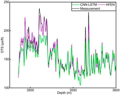
FIGURE 14. HFEN vs. Measurement in well 4.
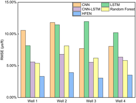
FIGURE 15. Comparison of predicted results (RMSE) between HFEN and other networks: CNN, LSTM, base CNN-LSTM, and random forest.
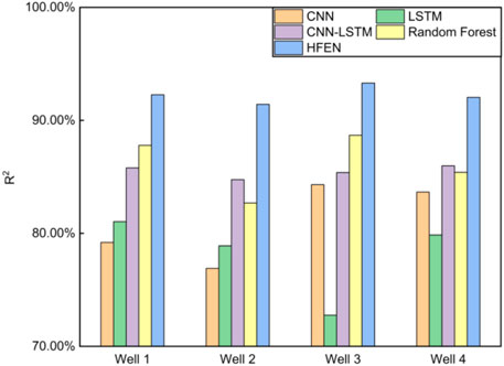
FIGURE 16. Comparison of predicted results (R2) between HFEN and other networks: CNN, LSTM, base CNN-LSTM, and random forest.
4 Conclusion
A novel multi-channel CNN-LSTM hybrid network is proposed in this study to improve acoustic log prediction in unconventional reservoirs where acquired data is often incomplete. To verify the performance of HFEN, the log data of Jimusar Shale Oilfield are taken as an example to conduct experiments and analyses. Compared with the actual measurement, the R2 of the four experiments are 92.27%, 91.42%, 93.31%, and 92.03%, and the RMSE are 3.32%, 3.92%, 3.06%, and 3.53%, respectively. This proves that the prediction is successful, and the predicted log has a high degree of similarity with the actual measurement log, which can accurately describe the formation properties and meet the subsequent engineering application requirements. All evaluation metrics of HFEN outperform the separate CNN and LSTM networks. The prediction results also demonstrate that the temporal and spatial features of the well logs are critical to the prediction accuracy, and HFEN can extract these two features effectively. The feature enhancement method boosts the input log features, to reflect fluctuating data trend and expand the feature space of the log to increase the diversity of log features for a small input sample size, thus improving the accuracy of the prediction. Future research will focus on the investigation into measurement-related physics processes to further enhance the feasibility of the current network as well as considering application towards other measurements, e.g., resistivity, nuclear, and NMR, to obtain a comprehensive evaluation of the reservoir and, therefore, reduce hydrocarbon exploration cost.
Data Availability Statement
The raw data supporting the conclusions of this article will be made available by the authors, without undue reservation.
Author Contributions
YH: methodology, conceptualization, writing original draft preparation. OL: original draft preparation. LS: data acquisition. ZL: data acquisition. QZ: supervision, writing, reviewing and editing. HW: reviewing and editing. YW: programming guidance. YZ: programming guidance.
Funding
The work was funded by the National Natural Science Foundation of China (Grant No. 52171253).
Conflict of Interest
The authors declare that the research was conducted in the absence of any commercial or financial relationships that could be construed as a potential conflict of interest.
Publisher’s Note
All claims expressed in this article are solely those of the authors and do not necessarily represent those of their affiliated organizations, or those of the publisher, the editors, and the reviewers. Any product that may be evaluated in this article, or claim that may be made by its manufacturer, is not guaranteed or endorsed by the publisher.
References
Ardabili, S., Abdolalizadeh, L., Mako, C., Torok, B., and Mosavi, A. (2022). Systematic Review of Deep Learning and Machine Learning for Building Energy. Front. Energy Res. 10. doi:10.3389/fenrg.2022.786027
Castagna, J. P., Batzle, M. L., and Eastwood, R. L. (1985). Relationships between Compressional‐wave and Shear‐wave Velocities in Clastic Silicate Rocks. Geophysics 50 (4), 571–581. doi:10.1190/1.1441933
Downton, J. E., Collet, O., Hampson, D. P., and Colwell, T. (2020). Theory-guided Data Science-Based Reservoir Prediction of A North Sea Oil Field. Lead. Edge 39 (10), 742–750. doi:10.1190/tle39100742.1
Du, Q., Yasin, Q., Ismail, A., and Sohail, G. M. (2019). Combining Classification and Regression for Improving Shear Wave Velocity Estimation from Well Logs Data. J. Petroleum Sci. Eng. 182, 106260. doi:10.1016/j.petrol.2019.106260
Eshkalak, M. O., Mohaghegh, S. D., and Esmaili, S. (2014). Geomechanical Properties of Unconventional Shale Reservoirs. J. Petroleum Eng. 2014, 1–10. doi:10.1155/2014/961641
Feng, R., Grana, D., and Balling, N. (2021). Imputation of Missing Well Log Data by Random Forest and its Uncertainty Analysis. Comput. Geosciences 152, 104763. doi:10.1016/j.cageo.2021.104763
Greenberg, M. L., and Castagna, J. P. (1992). Shear-wave Velocity Estimation in Porous Rocks: Theoretical Formulation, Preliminary Verification and Applications1. Geophys Prospect 40 (2), 195–209. doi:10.1111/j.1365-2478.1992.tb00371.x
Guo, X. G., He, W. J., Yang, S., Wang, J. T., Feng, Y. L., Jia, X. Y., et al. (2019). Evaluation and Application of Key Technologies of"Sweet Area"of Shale Oil in Junggar Basin:Case Study of Permian Lucaogou Formation in Jimusar Depression. Nat. Gas. Geosci. 30 (8), 1114. doi:10.11764/j.issn.1672-1926.2019.07.007
Hall, M., and Hall, B. (2017). Distributed Collaborative Prediction: Results of the Machine Learning Contest. Lead. Edge 36 (3), 267–269. doi:10.1190/tle36030267.1
Hochreiter, S., and Schmidhuber, J. (1997). Long Short-Term Memory. Neural Comput. 9 (8), 1735–1780. doi:10.1162/neco.1997.9.8.1735
Hu, X., Zhang, H., Ma, D., and Wang, R. (2021). A tnGAN-Based Leak Detection Method for Pipeline Network Considering Incomplete Sensor Data. IEEE Trans. Instrum. Meas. 70, 1–10. doi:10.1109/TIM.2020.3045843
Hu, X., Zhang, H., Ma, D., and Wang, R. (2021). Hierarchical Pressure Data Recovery for Pipeline Network via Generative Adversarial Networks. IEEE Trans. Autom. Sci. Eng., 1–11. doi:10.1109/TASE.2021.3069003
Kim, B. S., and Kim, T. G. (2019). Cooperation of Simulation and Data Model for Performance Analysis of Complex Systems. Int. J. Simul. Model. 18 (4), 608–619. doi:10.2507/IJSIMM18(4)491
Li, W., Qi, F., Tang, M., and Yu, Z. (2020). Bidirectional LSTM with Self-Attention Mechanism and Multi-Channel Features for Sentiment Classification. Neurocomputing 387, 63–77. doi:10.1016/j.neucom.2020.01.006
Li, Y., Sun, R., and Horne, R. (2019). Deep Learning for Well Data History Analysis,” in Proceedings - SPE Annual Technical Conference and Exhibition, Calgary, Alberta, Canada, September 2019. doi:10.2118/196011-MS
Lin, L., Luo, H., Huang, R., and Ye, M. (2019). Recurrent Models of Visual Co-attention for Person Re-identification. IEEE Access 7, 8865–8875. doi:10.1109/ACCESS.2018.2890394
Long, F., Zhou, K., and Ou, W. (2019). Sentiment Analysis of Text Based on Bidirectional LSTM with Multi-Head Attention. IEEE Access 7, 141960–141969. doi:10.1109/ACCESS.2019.2942614
Mehrad, M., Ramezanzadeh, A., Bajolvand, M., and Reza Hajsaeedi, M. (2022). Estimating Shear Wave Velocity in Carbonate Reservoirs from Petrophysical Logs Using Intelligent Algorithms. J. Petroleum Sci. Eng. 212, 110254. doi:10.1016/j.petrol.2022.110254
Mosavi, A., Ardabili, S., and Várkonyi-Kóczy, A. R. (2020). List of Deep Learning Models. Int. Conf. Glob. Res. Educ. 101, 202–214. doi:10.1007/978-3-030-36841-8_20
Pan, S., Zheng, Z., Guo, Z., and Luo, H. (2022). An Optimized XGBoost Method for Predicting Reservoir Porosity Using Petrophysical Logs. J. Petroleum Sci. Eng. 208, 109520. doi:10.1016/j.petrol.2021.109520
Pham, N., and Zabihi Naeini, E. (2019). “Missing Well Log Prediction Using Deep Recurrent Neural Networks,” in 81st EAGE Conference and Exhibition. doi:10.3997/2214-4609.201901612
Rehman, A. U., Malik, A. K., Raza, B., and Ali, W. (2019). A Hybrid CNN-LSTM Model for Improving Accuracy of Movie Reviews Sentiment Analysis. Multimed. Tools Appl. 78 (18), 26597–26613. doi:10.1007/s11042-019-07788-7
Shan, L., Liu, Y., Tang, M., Yang, M., and Bai, X. (2021). CNN-BiLSTM Hybrid Neural Networks with Attention Mechanism for Well Log Prediction. J. Petroleum Sci. Eng. 205, 108838. doi:10.1016/J.PETROL.2021.108838
Song, L., Liu, Z., Liu, Z., Li, C., Ning, C., Hu, Y., et al. (2021). “Prediction and Analysis of Geomechanical Properties of Jimusaer Shale Using a Machine Learning Approach,” in SPWLA 62nd Annual Logging Symposium, Virtual Event(online), May 2021. doi:10.30632/SPWLA-2021-0089
Wang, H., Ma, F., Tong, X., Liu, Z., Zhang, X., Wu, Z., et al. (2016). Assessment of Global Unconventional Oil and Gas Resources. Petroleum Explor. Dev. 43 (6), 925–940. doi:10.1016/S1876-3804(16)30111-2
Wang, J., Cao, J., You, J., Cheng, M., and Zhou, P. (2021). A Method for Well Log Data Generation Based on A Spatio-Temporal Neural Network. J. Geophys. Eng. 18 (5), 700–711. doi:10.1093/jge/gxab046
Wang, J., Cao, J., Zhao, S., and Qi, Q. (2022). S-wave Velocity Inversion and Prediction Using a Deep Hybrid Neural Network. Sci. China Earth Sci. 65, 724–741. doi:10.1007/s11430-021-9870-8
Wang, P., and Peng, S. (2019). On a New Method of Estimating Shear Wave Velocity from Conventional Well Logs. J. Petroleum Sci. Eng. 180, 105–123. doi:10.1016/j.petrol.2019.05.033
Wang, Y., Huang, M., zhu, x., and Zhao, L. (2016). “Attention-based LSTM for Aspect-Level Sentiment Classification,” in EMNLP 2016 - Conference on Empirical Methods in Natural Language Processing, Proceedings, Austin, Texas, January 2016. doi:10.18653/v1/d16-1058
Wang, Y., Zhang, X., Lu, M., Wang, H., and Choe, Y. (2020). Attention Augmentation with Multi-Residual in Bidirectional LSTM. Neurocomputing 385, 340–347. doi:10.1016/j.neucom.2019.10.068
Xie, Y., Liang, R., Liang, Z., and Zhao, L. (2019). Attention-based Dense LSTM for Speech Emotion Recognition. IEICE Trans. Inf. Syst. E102.D (7), 1426–1429. doi:10.1587/transinf.2019EDL8019
Yang, T., Li, Y., Pan, Q., and Guo, L. (2016). Tb-CNN: Joint Tree-Bank Information for Sentiment Analysis Using CNN. Chin. Control Conf. doi:10.1109/ChiCC.2016.7554468
You, J., Cao, J., Wang, X., and Liu, W. (2021). Shear Wave Velocity Prediction Based on LSTM and its Application for Morphology Identification and Saturation Inversion of Gas Hydrate. J. Petroleum Sci. Eng. 205, 109027. doi:10.1016/j.petrol.2021.109027
Zeng, L., Ren, W., Shan, L., and Huo, F. (2022). Well Logging Prediction and Uncertainty Analysis Based on Recurrent Neural Network with Attention Mechanism and Bayesian Theory. J. Petroleum Sci. Eng. 208, 109458. doi:10.1016/J.PETROL.2021.109458
Zhang, D., Chen, Y., and Meng, J. (2018). Synthetic Well Logs Generation via Recurrent Neural Networks. Petroleum Explor. Dev. 45 (4), 629–639. doi:10.1016/S1876-3804(18)30068-5
Zhang, Y., Zhang, C., Ma, Q., Zhang, X., and Zhou, H. (2022). Automatic Prediction of Shear Wave Velocity Using Convolutional Neural Networks for Different Reservoirs in Ordos Basin. J. Petroleum Sci. Eng. 208, 109252. doi:10.1016/J.PETROL.2021.109252
Zhou, T., Canu, S., Vera, P., and Ruan, S. (2021). Feature-enhanced Generation and Multi-Modality Fusion Based Deep Neural Network for Brain Tumor Segmentation with Missing MR Modalities. Neurocomputing 466, 102–112. doi:10.1016/J.NEUCOM.2021.09.032
Nomenclature
b Bias
bi-LSTM Bi-directional long short-term memory
BP Backpropagation neural network
CNN Convolutional neural network
ct Cell state
d A depth value of the log
DEN Density
DTC Compressional wave slowness
DTS Shear wave slowness
ft Forget gate
GR Natural gamma
GRU Gated recurrent unit
h Hidden state
i Number of different log types
it Input gate of lstm
JSO Jimusaer shale oilfield
layer Geological layer
LSTM Long short-term memory
max The maximum value of a sample value
min The minimum value of the sample value
RMSE Root mean square error
RNN Recurrent neural network
RT Deep resistivity
SSE The sum of squares of the errors
SST The sum of squares of the difference between the original data and the mean
STNN Spatio-temporal neural network
SVR Support vector regression
t Time
tanh Tanh activation function
w Weight
x Log sampling points
X Input sequential data
xgrad Log after gradient calculation
α Attention weight coefficient at different time
β Attention weight coefficients of different logs
σ Sigmoid activation function
Keywords: unconventional reservoir, hybrid neural network approach, acoustic data, CNN, LSTM
Citation: Hu Y, Li O, Song L, Liu Z, Zhang Q, Wu H, Wang Y and Zhang Y (2022) Acoustic Prediction of a Multilateral-Well Unconventional Reservoir Based on a Hybrid Feature-Enhancement Long Short-Term Memory Neural Network. Front. Energy Res. 10:888554. doi: 10.3389/fenrg.2022.888554
Received: 03 March 2022; Accepted: 02 May 2022;
Published: 13 June 2022.
Edited by:
Greeshma Gadikota, Cornell University, United StatesReviewed by:
Xuguang Hu, Northeastern University, ChinaSina Ardabili, University of Mohaghegh Ardabili, Iran
Copyright © 2022 Hu, Li, Song, Liu, Zhang, Wu, Wang and Zhang. This is an open-access article distributed under the terms of the Creative Commons Attribution License (CC BY). The use, distribution or reproduction in other forums is permitted, provided the original author(s) and the copyright owner(s) are credited and that the original publication in this journal is cited, in accordance with accepted academic practice. No use, distribution or reproduction is permitted which does not comply with these terms.
*Correspondence: Qiong Zhang, emhhbnFpb0B1ZXN0Yy5lZHUuY24=
†These authors have contributed equally to this work and share first authorship