A Possibilistic Risk Assessment Framework for Unmanned Electric Vehicles With Predict of Uncertainty Traffic

At present, electric vehicles (EV) have entered a stage of rapid development. Meanwhile, with artificial intelligence (AI) technology fast improving and implementing many inventions in electric vehicles (EV), almost all EV sold in China are equipped with automatic driving technology to achieve safer and more energy-saving driving. In order to solve the problem of anti-collision in self-driving Smart EV under complex traffic, especially at intersections, most of the existing methods make sequential predictions for the driving level of vehicles, and it becomes difficult to deal with sudden changes in intentions of other vehicles. Therefore, a collision risk assessment framework based on other vehicles’ trajectory prediction is proposed. The framework integrates the solutions of other vehicles’ expected path planning, uncertainty description of driving process, trajectory change caused by obstacle intrusion, etc., as well as adopts the Gaussian mixture model to evaluate the risk according to the probability of collision. It realizes the real-time evaluation of the probability of collision and makes safe decisions and trajectory planning of the vehicles. After simulation and verification, it effectively solves the decision-making planning problem of autonomous vehicles under complicated traffic flow and demonstrates that the method is better than the current sequential prediction method (SORT\Karlman filter, etc.).

1 Introduction

Crossroads are one of the traffic scenes with the most complicated driving conditions. For autonomous vehicles, it is of great significance to further improve and ensure vehicle safety if they can sense the intention of other vehicles in advance and predict possible collision risks between themselves and the other vehicles.

At present, in the problem of collision avoidance in autonomous driving scenes, the trajectory planning and behavior decision of autonomous driving vehicles mainly need to consider other dynamic obstacles in traffic scenes. At the same time, including but not limited to the driving trajectories of the other motor vehicles, to determine the behavior decision and trajectory planning of the autonomous driving vehicles. The two main methods in the industry for this are planning-based method and optimization-based control method. Trajectory planning is a typical control method which includes advance planning based on prior environmental information in addition to real-time planning based on online space exploration (Wang et al., 2019; Wang and Huang, 2021), aiming at finding an optimal free path of colliding vehicles. Trajectory planning and collision avoidance based on the potential field have also been widely studied (Gianibelli et al., 2018; Chen and Yu, 2019). This method avoids collision behavior based on the potential field and uses the potential field to push vehicles away from certain obstacles. Planning-based methods are faced with the challenge of designing suitable collision avoidance paths, and it is difficult to find suitable optimal paths for a complex dynamic road condition. On the other hand, optimization-based control method (MPC) (Rothmund and Johansen, 2019) is also widely used for collision avoidance of unmanned vehicles. Collision avoidance is regarded as a coupling constraint, and the best collision avoidance algorithm is found for vehicles. There are also some researchers who speculate the upper limit of collision probability of the minimum collision time TTC (Shalev-Shwartz et al., 2017) based on the linear space and time of trajectory crossing to constrain the behavior decisions of unmanned vehicles such as deceleration and braking. However, this does not take into account the uncertainty and conservatism of obstacles, nor does it take into account the risk in the sense of probability. In recent years, many researchers have used AI methods to study path planning and collision avoidance of unmanned vehicles in a complex dynamic scenario, including the reinforcement learning methods of RL (Q-Learning) (Zhao et al., 2017) and POMDP (Hsu et al., 2008; Ponzoni Carvalho Chanel et al., 2012; Ragi and Chong, 2013). According to environmental rewards, calculate possible actions and get the next step. Some work has been put forward for a POMDP solution to model the uncertainty of target trajectory. But this solution needs to consider a large number of possible action sequences and the state of other vehicles, which must be completed in an ideal time and consume a lot of system resources and computing power. RL methods may suffer from problems caused by overfitting due to the complexity of environment and various characteristics of tasks. At the same time, less environmental knowledge may slow down the learning speed and cause unmanned vehicles to fall into local optimum.

The main contribution of this article is to develop a framework based on the collision risk assessment for obstacle avoidance in an unknown environment. This method predicts the environment along with preplanned tracks of other vehicles and analyzes the uncertainties. It includes other vehicles’ expected path planning, uncertainty description of driving process, and trajectory change caused by obstacle intrusion. Through the analysis, modeling, and calculation of uncertainty, the prediction of other vehicles’ trajectory based on probability is realized. The risk probability of collision is evaluated based on the other vehicles’ trajectory. This result can be input to the decision control module for correcting or changing the motion planning of the own vehicle and can also trigger other safety algorithms of the own vehicle such as collision avoidance when necessary, moreover, ensuring vehicle safety to the greatest extent along with better driving efficiency.

2 Driving Uncertainty Analysis

Among the four factors that affect vehicle trajectory, the legal driving direction of the lane and geometric characteristics of the road are almost constant. This relevant information can be obtained through maps, high-precision maps, networks, or vehicle perception. The remaining three factors are uncertain with time and environment, which is the key and difficult point of other vehicles' trajectory prediction. It is also the key and difficult point of collision risk assessment. In this article, these three factors are summarized as three kinds of uncertainties that affect the trajectory of other vehicles and are analyzed, modeled, and calculated.

2.1 Uncertainty of Driving Intention

At present, the intelligent vehicle cannot accurately sense the driving intention of its driver, so the driving intention of its own vehicle is uncertain. As shown in Figure 1A, when turning around, turning left, going straight, and turning right are allowed in the lane in which other cars travel, the driving intention of the other cars is strongly uncertain when compared with that of the own car. Generally speaking, this uncertainty will decrease as the vehicle travels. For example, when a vehicle is at an intersection, there are possibilities of turning left, going straight, and turning around. When the vehicle travels halfway along the left-turn route, it can be judged that the vehicle is more likely to turn left. When the vehicle turns left and enters the other direction lane, the driving uncertainty disappears completely. Generally, an ego-vehicle’s driving intention will not change in a driving process, but in a few special cases, the driving intention may also change. As shown in Figure 1B, because the ego-vehicle is unfamiliar with the road environment or misreads the road signs, it may suddenly switch to the left turn after driving on the straight line for a period of time.

FIGURE 1

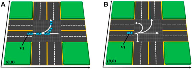
FIGURE 1. Example of driving intention uncertainty. (A) Lane has multiple legal driving directions. (B) Driver temporarily changes driving intention.

2.2 Driving Process Uncertainty

Because people’s perception, attention, operation ability, and other abilities cannot be as accurate as computers, and the vehicle’s power system and control system cannot control the vehicle absolutely accurately, there is always some uncertainty in the vehicle trajectory during the driving process. This kind of uncertainty is interfered by the external environment to a certain extent, for example, talking with the ego-vehicle will distract the driver’s attention, and fatigue driving will reduce the ego-vehicle’s driving ability. Another characteristic of this kind of uncertainty is that it only appears when the vehicle is moving and disappears naturally when the vehicle is stationary. This kind of uncertainty is called the uncertainty of driving process in this article. There are two types of uncertainties in driving process, each with different characteristics: the first type is mainly caused by the lack of ability of the drivers or vehicles, which is objective and inevitable. However, this kind of uncertainty is often small and occurs randomly near the true value of the driving intention; the second type is mainly caused by the ego-vehicle’s inattention. This kind of uncertainty may accumulate and enlarge and even eventually force drivers to change their driving intentions. For example, the vehicle originally wanted to go straight but because of the ego-vehicle’s mistake, the vehicle continued to turn left and finally entered the left-turn lane. At this time, the ego-vehicle had to temporarily change its driving intention to turn left.

2.3 Track Invasion Uncertainty

Due to the widespread existence of obstacles, vehicles often cannot drive according to the scheduled route, causing them to change the driving route constantly. However, obstacles may appear in any motion at any time and place, so the uncertainty caused by them is the most complicated and difficult to deal with. This kind of uncertainty is caused by external objects. In this article, it is called the uncertainty of other vehicles’ track invasion. Compared with the uncertainty of driving intention, obstacles appear to more frequently lead to a higher frequency of vehicle route change. Compared with the uncertainty of driving process, the change of driving trajectory caused by obstacle intrusion is bigger and more significant.

2.4 Trajectory Planning Analysis of Other Collision Avoidance Effects

In addition to the above factors and uncertainties, there are many factors that affect the driving of vehicles in reality. The most common of which are the right-of-way rules. The right-of-way rules stipulate the priority right-of-way of different vehicles on the same road in a specific scene. The right-of-way division affects the running of vehicles and thus the assessment of collision risk. Based on the actual driving situation, this article focuses on the influence of vehicle arrival time, vehicle type, and vehicle driving intention on the right of way. In this article, it is determined that when a vehicle arrives at a certain position at different times, the vehicle that arrives first enjoys the right of way, and the vehicle that arrives later should give way; when the vehicle arrives at a certain position at the same time, consider the driving intention of the vehicle, such as turning left and right should be straight; and if two cars have exactly the same right of way, they are in a constant competitive state, and the vehicles stop at random for a period of time and then compete for the right of way again.

Besides the right of way, when vehicles avoid each other, it also affects each of their driving. In order to make the calculation easy to realize, when predicting the driving track of other vehicles V_i, only the influence of the remaining vehicles on V_i is considered while the influence of V_i on the other vehicles is not considered. For example, if the driving track of V_i is invaded by V_j, V_i may change the driving route to avoid V_j. At this time, the influence of the V_i route change on V_j is no longer considered. If V_j is affected by V_i and the driving route is adjusted, the influence of V_j on V_i after changing the route should be reconsidered. So repeated recursion will fall into an infinite loop.

3 Implementation of Risk Assessment Framework

The calculation process of the risk assessment framework proposed in this article can be divided into three steps as a whole, as shown in Figure 2. The framework needs the injection of the sensing module and the driving track of the vehicle generated by the decision control algorithm in the future. The calculation results of the risk assessment can be returned to the decision control module for correcting or reestablishing the new driving track. Other safety algorithms can also be triggered when necessary such as directly starting the collision avoidance system when the collision probability is high. The whole calculation process needs to be iterated in real time while driving according to the changed environments.

FIGURE 2

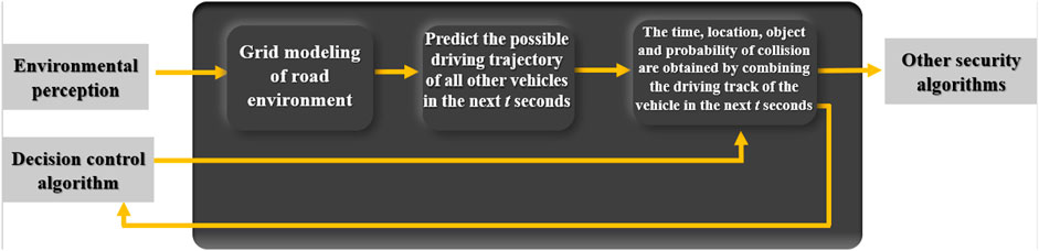
FIGURE 2. Overall calculation process of risk assessment framework.

3.1 Grid Modeling of Road Environment

The first step of calculation is to realize the perception of the surrounding environment. In order to facilitate the calculation, this article uses a two-dimensional coordinate system to realize the gridding description of the whole environment space. As shown in Figure 3, Figure 3A is a realistic intersection simulation diagram, while Figure 3B is a gridded coordinate space. The origin of the coordinate system can be chosen arbitrarily when gridding. It only affects the calculation process and does not affect the calculation result. In Figure 3, the lower left corner is taken as the origin of coordinates.

FIGURE 3

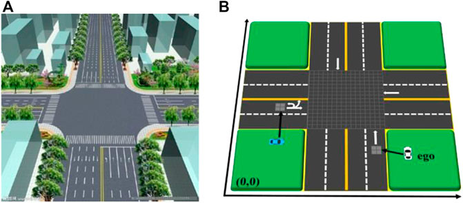
FIGURE 3. Road space gridding at crossroads. (A) Intersection simulation Ddiagram. (B) Intersection grid modeling results.

3.2 Uncertainty Modeling of Other Vehicles’ Trajectory

The second step is the focus of the whole calculation. It needs to deal with the three kinds of uncertainties mentioned above. Let the current time be t and the interval of iterative calculation be ∆t. Then, the evaluation of the risk of collision between the own vehicle and other vehicles in the next n cycles has to be done. Let us assume that there are n other cars at the current intersection and take any other car V as an example to explain the prediction and calculation process of its driving track in the intersection.

The essence of distribution probability lies in quantifying the uncertainty of driving intentions of various vehicles. This method holds that the probability distribution of the expected route is mainly affected by two factors: first, the statistical results of historical driving records, and second, the vehicle’s trajectory in the past period of time. As shown in Figure 4, let the vehicle drive from s to S₀ and enter the intersection at S₀. When the vehicle is located at S₀, because the driving track from S to S₀ is not helpful in distinguishing and identifying the driving intention of the vehicles, the probability of the vehicles traveling on various paths can be quantified more accurately by using historical statistical data. When the vehicle is located in S₁, it can be considered that the possibility of turning around decreases while the probability of turning left along P₂ and going straight along P₃ increases. When the vehicle is located at S₂, it can be considered that the probability of turning around and going straight continues to decrease and the probability of turning left along P₂ increases. When the vehicle is located at S₃, it can almost be considered that the vehicle will definitely turn left. When the vehicle finally arrives at S₄, it turns left. After the turn is completed, the driving intention of the vehicle is determined to turn left, and the uncertainty is completely eliminated.

FIGURE 4

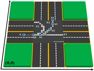
FIGURE 4. Example of vehicle driving.

K possible driving paths are planned when the vehicle V enters the intersection. Assuming that a total of N vehicles have passed from the S₀ position in the past period of time, and the number of vehicles traveling along route I is N_i, the driving probability $P_{\text{i}}=N_{\text{i}}/N$ can be assigned to route P_i, and when the vehicle travels along the expected path, the uncertainty of driving intention can be estimated and quantified by using the driving trajectory in the past period of time. As shown in Figure 5, the vehicle enters the intersection from S₀, and arrives at S₁ after driving for a period of time, with a driving distance of L. As P₂ and F₃ completely overlap in the L part, the process from S₀ to S₁ can be considered as follows: the vehicle has traveled a distance of L length along P₂, traveled a distance of L along P₃, and a distance of 0 along P₁. Theoretically, the probability of different expected paths of vehicles can be calculated by using the following formula:

$\begin{array}{l}N={\displaystyle {\sum }_{i=1}^K{N}_i},1={\displaystyle {\sum }_{i=1}^K{P}_i}\\ \{\begin{array}{l}{P}_{\text{around}}=\frac{0}{L+L+0}\\ P_{\text{left}}=\frac{L}{L+L+0}\\ P_{\text{straight}}=\frac{L}{L+L+0}\end{array}\end{array}(1)$

FIGURE 5

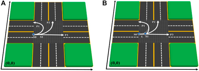
FIGURE 5. Calculate the expected path probability by using the traveled trajectory. (A) Vehicle initial position S_O. (B) Vehicle driving to S₁.

However, the above formula is prone to the extreme case of zero probability, which is inconsistent with the reality. Because even if the vehicle is located in S₁, there is still a certain probability of turning around, but this probability is smaller than turning left and going straight. Therefore, the above formula is adjusted based on Laplace’s smoothing idea to avoid the situation that the probability is 0 or 1. The adjusted formula is as follows:

$\{\begin{array}{l}{P}_{\text{around}}=\frac{0+1}{L+1+L+1+0+1}\\ P_{\text{left}}=\frac{L+1}{L+1+L+1+0+1}\\ P_{\text{straight}}=\frac{L+1}{L+1+L+1+0+1}\end{array}(2)$

The formula can be extended to the general situation, if the vehicle has k possible driving intentions at a certain position at the intersection, and the driving distance under the guidance of the i-th driving intention in the past period is L_i, the driving probability of the corresponding path under each intention in the future period is

$P_{\text{i}}=\frac{L_{\text{i}}+1}{{\displaystyle {\sum }_{i=1}^{K}L}+K},1={\displaystyle {\sum }_{i=1}^K{P}_{\text{i}}}(3)$

The above method can deal with the general case of path probability allocation, but there are two special cases to be explained: 1) when a vehicle enters an unplanned location for some reason, the distance from the previous location to the current location should be specially treated when calculating; 2) some planned routes may disappear and some new planned routes may come into being during the driving process of the vehicles.

As shown in Figure 6, when the vehicle is located at S₁, it should arrive at S₂ at the next moment according to the planned expected route. However, due to some reasons, such as the ego-vehicle’s inattention or obstacles at S₂, the vehicle actually enters S₃ at the next moment. However, the distance from S₁ to S₃ does not belong to any path among P₁, P₂, and P₃, so there will be ambiguity when using the above formula to calculate the probability. In order to ensure the smoothness of calculation, this article stipulates that d should be added to all L_i in this case, and the expected path of the vehicle should be replanned at the next moment.

FIGURE 6

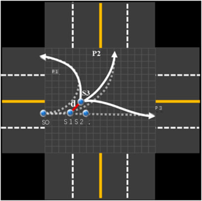
FIGURE 6. Vehicle driving into unplanned location.

In the second case shown in Figure 7, when the vehicle is in S₀, three expected paths are planned, namely P₁, P₂ and P₃. When the vehicle travels to S₁, because the direction of the front of the vehicle changes, the target area corresponding to P₁ is no longer visible (not within the 180-degree visual field), so P₁ disappears from the expected path and P₄ becomes the new expected path. At S₀, because the traffic rules stipulate that the inner lane is not allowed to turn right, there is therefore no driving intention to plan a right turn; at S₁, with the gradual exposure of the ego-vehicle’s driving intention, it is more and more possible for the vehicle to turn right, so a right-turn path is added. Since there is no P₄ path in the process from S₀ to S₁, the right turn probability cannot be calculated by the above formula. It is stipulated in this article that the probability of the disappearing path is no longer calculated, the initial probability of a new route is calculated.

FIGURE 7

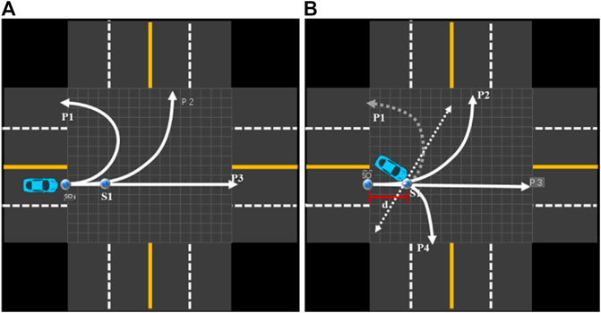
FIGURE 7. Add and delete expected paths. (A) Vehicle initial position. (B) Replanning path with change of head direction.

When calculating the expected path probability, it is not necessary to calculate the entire driving distance of the vehicle at the intersection. A time window can be set, and only the driving conditions within the time window can be considered, for example, only the driving conditions of the vehicle in the past 3 s can be considered.

Driving intention describes the uncertainty of vehicle trajectory from a macro perspective, while driving process describes the uncertainty of vehicle trajectory from a micro perspective. For the gridded intersection, the driving process of vehicles is equivalent to entering from one grid to another. Since the vehicle can travel to any feasible position in theory, it is also possible to enter a cell from any direction. As shown in Figure 8A, the vehicle may enter s from any direction of d1–d8. Similarly, as shown in Figure 8B, the vehicle may leave a cell from any angle. The essence of driving process uncertainty modeling is to measure the probability of leaving S from S along D₁–D₈. The traveling direction of the vehicle is controlled by the steering angle of the front wheel, and the direction of entering S affects the steering angle when the vehicle leaves. Therefore, the uncertainty modeling of driving process should consider both the direction when the vehicle enters and the direction when the vehicle leaves.

FIGURE 8

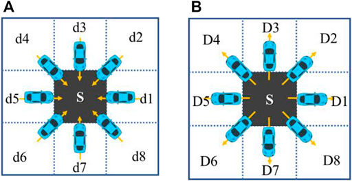
FIGURE 8. Entry and exit of vehicles relative to a certain cell. (A) Enters a cell in any direction. (B) Leaves a cell in any direction. Definition: L4 = d, with Pright = $\frac{L_4+1}{{\displaystyle {\sum }_{i=1}^{K^{\prime }}{L}_{\text{i}}+K^{\prime }}}$.

Uncertainty can be considered as random error based on driving intention. As shown in Figure 9, the actual trajectory of straight vehicles is often not an absolute straight line but an up-and-down disturbance. In this article, Gaussian distribution is used to describe the uncertainty of driving process. The sample of distribution is the steering angle of the vehicle, that is, the deflection angle of the front wheel during steering. In this article, negative values are used to indicate left turn, while a positive value indicates a right turn. For example, −3 means 3° to the left, +3 means 3° to the right, and 0° means straight without deflection. For Figure 9, the corresponding steering angle distribution during driving is shown in Figure 10.

FIGURE 9

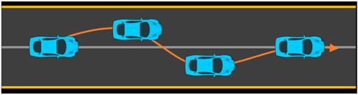
FIGURE 9. Possible driving results around the intention of going straight.

FIGURE 10

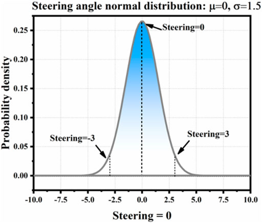
FIGURE 10. Example of Gaussian distribution of the steering angle when going straight.

There are two main reasons for describing the uncertainty of driving process with Gaussian distribution: 1) Gaussian distribution is a continuous distribution, and the steering angle which determines driving intention is taken as the distribution mean value, which can not only show the characteristics that the steering angle mainly changes around the mean value during driving but also allow the vehicle to deflect to any other direction, and the greater the deviation from the mean value, the smaller the probability. 2) Gaussian distribution is symmetrical about the mean, and its sampling probability on both sides of the mean is equal. This shows the randomness of driving deviation. As shown in Figure 9, the vehicle may shift above or below the centerline.

When the vehicle has only one expected path direction at the next moment, the steering angle distribution during driving from the current position to the next position can be described by Gaussian distribution, but there is often more than one expected path direction. This article uses Gaussian mixture distribution to deal with this situation. As shown in Figure 11A, when the vehicle is at S₁, there are three possible potential paths. Therefore, it is feasible to enter the next position from S₁ in three directions: D₂, D₁, and D₈. Let the probabilities in all directions be P₂, P₁, and P₈, and their specific values can be calculated by the method in the path probability allocation, in the previous section. Firstly, the steering angle distributions in the D₂, D₁, and D₈ directions are modeled, and the corresponding deflection angles are, respectively, μ₂, μ₁, and μ₈. The variance of the corresponding Gaussian distribution is σ₂, σ₁, and σ₈, so the steering angle Gaussian mixture model in the next period from S₁ is shown as follows, with its corresponding distribution graph shown in Figure 12:

$\{\begin{array}{l}P\left(X\right)=P_{2}G({\mu }_2,{\sigma }_2)+P_{1}G({\mu }_1,{\sigma }_1)+P_{8}G({\mu }_8,{\sigma }_8)\\ 1=P_2+P_1+P_8\end{array}(4)$

FIGURE 11

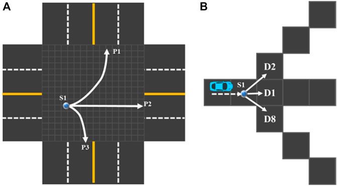
FIGURE 11. The vehicle has multiple expected driving directions. (A) Vehicle with multiple expected driving paths. (B) Vehicle with multiple expected driving directions.

FIGURE 12

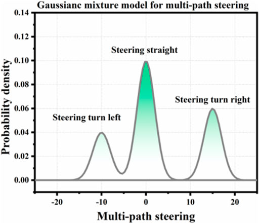
FIGURE 12. Probability distribution of Gaussian mixture model corresponding to the steering angle.

Although the probability is assigned to each expected path (the sum of the probabilities of each path is 1), this result cannot be directly used to measure the probability of vehicles traveling in all directions. Because under this result, the probability of the vehicle traveling beyond the expected direction is 0. As shown in the following figure, theoretically, there is only one expected S₂ direction in Figure 13, but in practice, the vehicle may still drive up to the light blue position. Combined with the uncertainty of driving process, this article uses the steering angular distribution function to calculate the driving probability of vehicles in all directions.

FIGURE 13

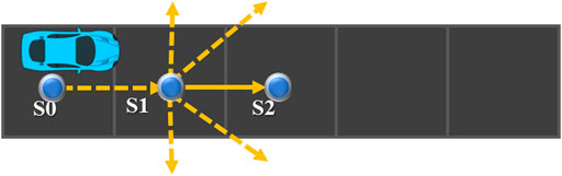
FIGURE 13. Single expected driving direction.

As shown in Figure 14A, when the vehicle is located at S₁, there are three possible paths, namely D₂, D_I, and D₈. However, due to the uncertainty of the driving process, there is a certain probability that the vehicle will drive in the D₃ and D₇ directions. As shown in Figure 14B, taking the 180-degree visual field in the front direction as all possible driving directions, the corresponding angles of D₁, D₂, D₈, D₇, and D₃ are α, β, and γ. If the side length of the cell square is 2, then $\sin \alpha =1/\sqrt{10},\alpha =\arcsin (1/\sqrt{10})$ The (radian) angle is about 18.4° (−90° to −72°, 72°–90°). According to the cosine formula of a triangle, $\beta =\arccos (a^2+b^2-c^2/2ab)$, then $\beta \approx 0.93$; it is about 53.1° (−72° to −19°, 19°–72°).

FIGURE 14

FIGURE 14. Multiple expected driving directions and distribution angles. (A) Multiple expected driving directions. (B) Corresponding angle of expected driving direction.

According to α, β, there is γ ≈ 0.66, which is about 38° (−19°, 19°). After calculating the values of α, β, and γ, combined with the probability density function of Gaussian mixture distribution, the corresponding probability areas at different angles can be obtained, which can be used as the probability of the vehicle traveling in this direction.

According to the above calculation results, the value of β is larger than α and γ, which is because the direction angles of D₂ and D₈ are larger than those of D₁, D₃, and D₇ in this scheme. The values of α, β, and γ can be adjusted according to the actual situation, or the variance value can be adjusted in the corresponding Gaussian distribution, to correct the probability of vehicles traveling in all directions. Generally speaking, the values of α, β, and γ and the variance of Gaussian components corresponding to each direction can be set as required or can be obtained by simulation and statistics according to the real situation. Let the probabilities of the preset directions D₂, D₁, and D₈ in Figure 14A be 0.2, 0.5, and 0.3, respectively, in which the variance of Gaussian distribution in D₁, D₃, and D₇ is 1.5, and the variance of Gaussian distribution in D₂ and D₈ is 2. The values of the corresponding steering distribution and the corresponding distribution of α, β, and γ are shown in Figure 15. In this example, the probability areas in the D₃ and D₇ directions corresponding to angle A are very small, so they are almost invisible in the figure.

FIGURE 15

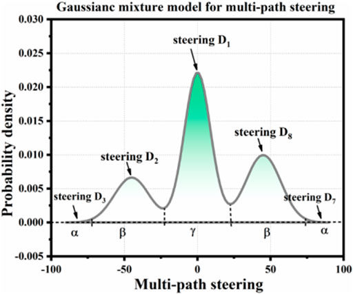
FIGURE 15. Steering unmixing Gaussian distribution function image.

Since the vehicle may enter a certain cell (position) from any direction, the probability of the vehicle arriving at a certain cell at time t is the sum of the probabilities of entering the cell in all directions, which can be used for the evaluation of the later collision risk. When the vehicle arrives at the t+∆t time position from the t time position, its probability calculation includes two steps: 1) based on the direction of the vehicle entering the current cell at time t, the probability of entering the next cell from this direction is calculated. In this calculation, firstly, we were required to establish the steering distribution based on the driving direction, and then use the steering distribution to calculate the probability of going to the next cell and multiplying it with the probability of entering the cell at t time. 2) Iterative calculation, always entering the current cell in all directions and driving into the next cell at t+∆t, and accumulating all the probabilities of reaching a certain cell at t+∆t to obtain the final probability of entering the cell at t+∆t.

As shown in Figure 16, if the vehicle could enter s from d₄, d₅, and d₆ directions at time t and their respective probabilities be P_d4, P_d5, and P_d6, the final probability of the vehicle reaching s at the moment of anti-engraving is P_s = P_d4 + P_d5 + P_d6, which in calculating the position and probability of time t+∆t is according to the calculation steps introduced above:

FIGURE 16

FIGURE 16. Entering and leaving a cell in multiple directions.

1) Firstly, based on the situation that the vehicle enters s based on d₅ direction, the expected driving direction of the vehicle at t+∆t time is only D₁ and the expected deflection angle of the vehicle when entering s from d₅ and leaving along D₁ is 0°. Therefore, the steering distribution of the vehicle in this case is a single Gaussian distribution with a mean value of 0. Let the standard deviation of the Gaussian distribution be assumed to be 16 (which can be set according to actual statistical results or simulation results in specific application), then the steering distribution of t time entering s along d₅ and t+∆t time leaving s along D₁ is shown in Figure 17. Under this distribution, the probability distribution of vehicles leaving S along D₁, D₂, D₈, D₃, and D₇ is the probability area of the steering distribution at the corresponding angles (the angles corresponding to each direction have been calculated and explained in the previous section), which is calculated as P_d1 ≈ 0.765, P_D2 = P_D8 ≈ 0.118, and P_D3 = P_D7 ≈ 0. Here, the sum of P_D1, P_D2, and P_D8 is greater than 1 due to rounding, not calculation error. The value of P_D3, P_D7 is 0 because of the limited calculation accuracy. Theoretically, their values are all greater than 0. Based on the above results, it can be obtained that the probability of the vehicle entering S from d₅ at t time and entering S₁ at t+∆t time is P_S1 = P_d5 × P_d1; the calculation of S₂, S₈, S₃, and S₇ is entered and then analogized to P_si = P_di × P_Di.

FIGURE 17

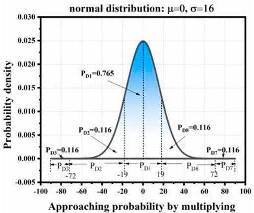
FIGURE 17. Gaussian distribution of vehicles when D₅ enters D₁ and leaves. and leaving along D₁ direction, which corresponds to P_D1 in the previous example.

2) Because it is possible for a vehicle to enter S from d₄, d₅, and d₆, the probabilities of entering S₁ at t+∆t are calculated in these cases, the probability of the vehicle at S₁ at t+∆t is the cumulative sum of the probabilities in all cases, $P_{S_1}^{t+\Delta t}={\displaystyle \sum P_{\left(S,di\right)}^t{P}_{Dj}^{di}}$, where $P_{S_1}^{t+\Delta t}$ means the probability of reaching S₁ at time t+∆t, $P_{(S,di)}^t$ indicates the probability of reaching S along di direction at time t, which corresponds to P_d5, P_d4, and P_d6 in Figure 16. In the above example, $P_{Dj}^{di}$ indicates the probability of entering S along the di direction.

Combining the above two calculation steps, based on the uncertainty of path planning and driving process, the probability formula of the vehicle arriving at S at t time is as follows $P_S^t={\displaystyle \sum _{i=1}^8{P}_{di}^t}$. The result can be used to evaluate the risk of collision at time t and position S. At t+∆t, the probability of the vehicle arriving at Sj is as formula, P^di_Dj is the path probability according to the planned path, the steering distribution of driving vehicles leaving S at time t is obtained, and then the probability area of the corresponding direction is obtained by using the distribution function.

In theory, vehicles can travel to any position in any direction, which not only makes trajectory prediction difficult but also increases the amount of calculation greatly. However, through analysis, it can be found that most of the calculations are at a very low level of probability. Therefore, this part of the calculations is almost meaningless to the final risk assessment and can be optimized by probability pruning and truncation (to reduce the calculation amount and improve calculation efficiency). As shown in Figure 18, dark green is the expected driving direction of the vehicle, that is, the planned path direction, while the other directions are unexpected driving paths caused by the uncertainty of driving process. If the probability of driving from the current cell to the next cell on the expected path decreases by 0.6 times, the probability of reaching a specific cell from t₁ to t₄ becomes 0.6, 0.36, 0.216 and 0.130, respectively. These probability values correspond to the most likely driving path of the vehicle, which is very valuable for risk assessment. However, under the other two paths, the probability value decreases exponentially and quickly drops to a very low level, such as 0.0001 > 0.00001, etc., and the probability value will only be lower after further calculation. In theory, the probability value of reaching any position at any time will be very low but not zero, but the probability value below a certain level is almost meaningless for practical application. If a collision probability of 0.00000000001 is evaluated, it can be almost considered that the collision will not occur. In this article, the threshold R_low is set as the minimum value of probability pruning truncation. When R_low is less than or equal to, the calculation will be cut off to reduce the amount of calculation. As shown in Figure 18, it can be set that when the probability of the vehicle arriving at s = 0.0001, the probability of leaving from S and arriving at the new cell at t5 will no longer be calculated.

FIGURE 18

FIGURE 18. Very low probability value of unexpected direction.

Probability truncation can not only reduce the amount of calculation but also avoid many meaningless calculations. As shown in Figure 19, the expected path of the vehicle is marked by dark green, but it is possible for the vehicle to enter the upper right cell at t₂ under the driving process uncertainty. Then, under the influence of driving process uncertainty, the vehicle may form a circle along the diamond; as shown in the figure, the gray arrow indicates the direction. This situation can continue indefinitely with the expansion of the time window, but under normal circumstances, almost no driver will drive the vehicle around the intersection.

FIGURE 19

FIGURE 19. Vehicle running in loop.

A direct manifestation of probability truncation is that the sum of probabilities of vehicles arriving at all positions at time t is less than 1 (without considering the loss of calculation accuracy and rounding), and the value of probability sum will gradually decrease with time. As shown in Figures 20A–C, the vehicle enters S at time t along the straight direction, theoretically departs from S, and reaches S_i, S₂, S₃, S₈, and S₇ at t₁. Let the probability be P₁–P₈. If only S_L, S₂, and S₈ are left to reach after probabilistic pruning, then the sum of probabilities of vehicles arriving at each feasible position at t₁ is the sum of P₁, P₂, and P₈, which is obviously less than the sum of P₁–P₈ and less than 1, which is the probability loss caused by pruning and truncation. Furthermore, the theoretically accessible positions at t₂ and S₁, S₂, and S₈ are shown in Figure 20E. After pruning, only the cells as shown in Figure 20F are left. The probability values of all accessible positions of the vehicle at t₂ are also determined by P₁′–P₈′. The sum becomes P₁′, P₂′, and P₉′. In addition, there is a probability loss. The loss of probability can be understood as the cost of precision due to reducing the amount of calculation.

FIGURE 20

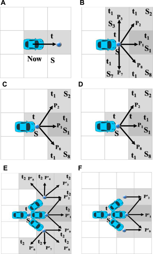
FIGURE 20. Pruning and truncation of vehicle running probability. (A) t time entry diagram. (B) All feasible directions at t₁. (C) Feasible direction after pruning at t₁ time. (D) Possible position at t₁. (E) All feasible directions at t₂. (F) Feasible directions after pruning at t₂.

The uncertainty of driving intention and driving process mainly aims at the uncertainty of vehicle interior and driver, while the uncertainty of trajectory invasion focuses on the impact of real-time change of the external environment on vehicle trajectory. When obstacles (possibly, motor vehicles, bicycles, motorcycles, pedestrians, suddenly dropped goods, etc.) intrude into the expected driving position of the vehicle, the vehicle will be forced to respond, such as make detours and stops, all of which will change the vehicle’s trajectory and thus change the time, location, and probability of collision with the vehicle.

In this article, we define trajectory intrusion from two aspects of time and space. In time, it includes the current time or future time in the time window. In space, it refers to the position where the current or future time of the obstacle overlaps with the possible entry position of other vehicles. As shown in Figure 21, if the other vehicle is located at s at the current moment, it may drive along D₁, D₂, D₃, D₄, and D₅ directions. The barrier is located at S₄, and it could be heading for S₃ at the next moment. When other vehicles drive into S₄ from S along the direction of D₄ because the position of obstacles at the current moment overlaps with the possible driving position of other vehicles at the next moment, the track of the other vehicles at S₄ is invaded at the next moment. When other vehicles enter S₃ from S along the direction of D₃, it is possible to drive into S₃ at the next moment due to obstacles. Therefore, the track of its car in S₃ is also invaded at the next moment. In short, if the obstacle is located at A at the moment, and if other vehicles drive to A at the next moment, then A is considered as a trajectory intrusion; if the obstacle and other vehicles are likely to drive to point B at the next moment, then point B is also a trajectory intrusion. In some special cases, such as different rights of way classes between vehicles, it can be considered that the tracks of vehicles with a higher right of way will not be invaded because they enjoy the right of way. At this time, only the tracks of vehicles with a lower right of way are invaded.

FIGURE 21

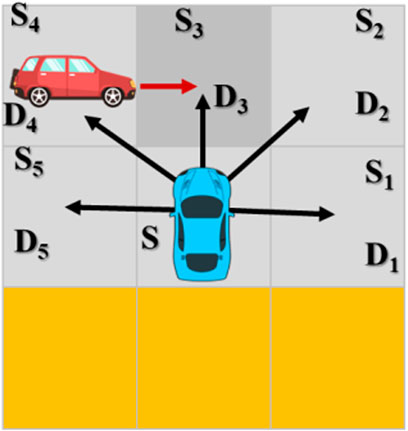
FIGURE 21. Example of trajectory intrusion.

When encountering the track invasion, the actions taken by the vehicle is to stop and wait, that is, the vehicle stays still at the current position until the obstacles leave and then resumes driving, or detour, that is, the vehicle does not stop but travels in a nonintrusive direction to bypass the obstacle. Trajectory intrusion changes the route of vehicles, and the route and its probability are determined by path planning and steering distribution. Therefore, the trajectory intrusion will change the original steering distribution of the vehicle and the probability of driving along each direction. When a vehicle enters the next cell with a probability greater than the cutoff probability, it may be necessary to delete or add new paths and reallocate the probability of each path. So, trajectory intrusion uncertainty modeling should be combined with path planning and steering distribution to quantify different situations.

Here, the probability of obstacles reaching the intrusion position is taken as the rejection rate, and the steering distribution is regenerated by the rejection sample. As shown in Figure 22A, at time t, other vehicles are located at S, obstacles are located at S₄, and obstacles may be located at S₃ at the next time. S₄ and S₃ are both the positions where the tracks of other vehicles are invaded at the next moment. Let it have three expected driving directions, say D₂, D₃, and D₄ and the distribution probabilities of the three expected paths are P_D4 = 0.3, P_D3 = 0.5, and P_D2 = 0.5, respectively, and their steering distribution is shown in Figure 22B. It can be seen that the probability areas in the D₃ and D₄ directions are large and the driving process in the D₄ direction is uncertain, so the Gaussian distribution variance in the steering D₄ area is large, and it is “stout” on the graph. D₅ and D₁ are not preset directions, therefore, the corresponding probability area is small, and the eye flesh is almost invisible.

FIGURE 22

FIGURE 22. Obstacle intrusion and original steering distribution of vehicles. (A) Expected driving direction of vehicles and position of obstacle intrusion. (B) Original steering distribution of vehicles.

Let the probabilities of obstacles reaching S₄ and S₃ at time t be P₀₁ = 0.7 and P₀₂ = 0.6, respectively, and P₀₁ and P₀₂ are D₄, sampling steering with rejection rate in the D₃ direction, and relearning steering distribution with sampled samples as shown in Figure 23. In the figure, the red dotted line indicates the steering distribution before rejecting sampling, and the blue solid line indicates the new steering distribution learned after rejecting sampling. It can be seen from the figure that the probability areas in the D₄ and D₃ directions decrease to a certain extent, while the probability areas in the D₂ direction increase greatly. The probability areas in D₁ and D₅ directions increase slightly.

FIGURE 23

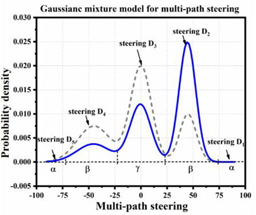
FIGURE 23. Newly generated steering distribution after rejecting sampling.

Although the new steering distribution can be obtained by taking the probability of obstacles reaching a certain position as the rejection rate, the simulation test shows that the discrimination between many new distributions and the old distributions is not obvious enough. As shown in Figure 24, let the arrival probabilities of obstacles in Figure 24A be P₀₁ = 0.3 and P₀₂ = 0.2, and the distribution probabilities of vehicles along the planned paths D₄, D₃, and D₂ before sampling rejection be P_D4 = 0.3, P_D3 = 0.5, and P_D2 = 0.2. With P₀₁ and P₀₂ as rejection rates, the obtained steering distribution after sampling is shown in Figure 24B, and the curve difference between before-sampling and after-sampling is not obvious. Especially, along the D₃ direction, the probability of the vehicles entering is hardly affected by obstacles, but in fact, P₀₁ = 0.3 and P₀₂ = 0.2 are already relatively high probability values. This shows that it is not enough to show the influence of obstacles on the driving track by directly using the probability of arrival of obstacles as the rejection rate. In this article, it is considered that squeeze operation can be performed according to a certain mapping rule P_oi, to realize the influence of obstacles on the vehicle trajectory.

FIGURE 24

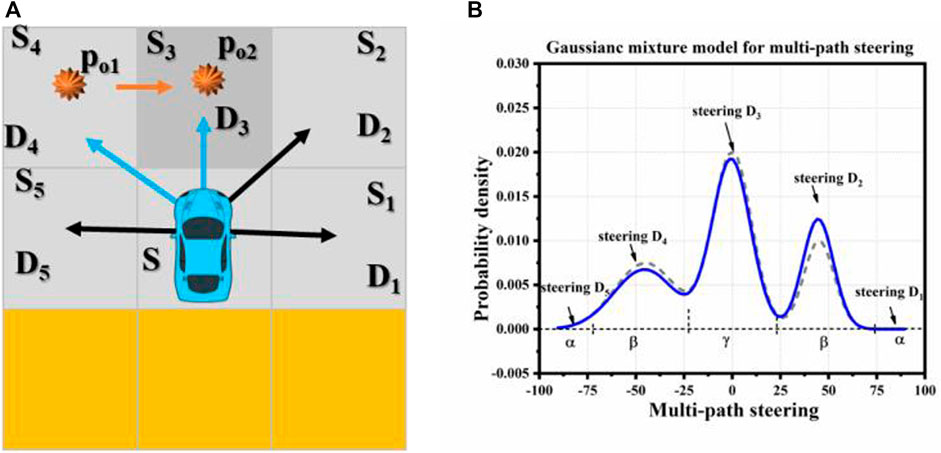
FIGURE 24. There is no obvious difference in the distribution of new and old steering. (A) Expected driving direction of vehicles and position of obstacle intrusion. (B) New and old steering distribution.

The squeeze mode can be flexibly selected according to the situation. For example, the analytic equation of a circle can be the squeezed function, and the value curve of P_oi can be extruded into the circular arc shape. As shown in Figure 25A, the red straight line is the original P_oi, according to the equation of circle, (x − 1)² + y² = 1 y = √(1 − (x − 1)²). The rejection rate after Squeeze is shown as the blue curve. Figure 25B shows the steering distribution generated by the rejection rate sampling after squeeze, which shows that the distribution difference is more obvious. Except for the equation of the circle, other functions that map P_oi to the range of 0–1 can be used as squeeze functions, such as deformed log function, logistic function, sigmoid function, etc., and the rejection rate is amplified in different ways by different functions. To influence the new steering distribution.

FIGURE 25

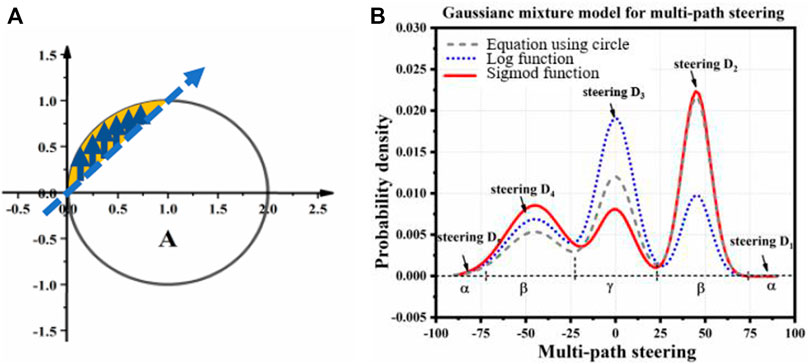
FIGURE 25. Squeeze the arrival rate of obstacles to get the rejection rate. (A) Squeeze the equation of a circle (B) Squeeze the steering distribution.

It is also a common in driving to choose to stop when facing obstacles, so it is necessary to allocate probabilities between stopping and detouring. Let ∆t be the time of iterative calculation of risk assessment, P_wait, P_bypass, then there is 1 = P_wait + P_bypass, indicating that it is possible for other vehicles to stop moving in the next time. In reality, the probability of stopping is related to the distribution of obstacles. If the possibility of obstacles invading the track is high or more positions in the track are invaded by obstacles, the possibility of stopping and so on will increase accordingly. As shown in Supplementary Figure S1, there are five possible driving directions within the visual field of other vehicles 180, and the probability of each direction can be obtained from the steering distribution before it refuses to sample, which is set as P_D1–P_D5. In extreme cases, these five directions may be invaded by obstacles. Let the invasion probability be P₀₁–P₀₅. If the values of P₀₁–P₀₅ are all 1, it is determined that the vehicle will be surrounded by obstacles at the next moment, then the probability of the vehicle stopping at this time is 1 to ensure driving safety. If the values of P₀₁–P₀₅ are all 0, it is determined that no obstacle will invade the trajectory of the other vehicles at the next moment. Then, the probability of the vehicle stopping should be 0, which accords with the driving habits of people. Because P_D1–P_D5 are calculated from the same steering distribution, there are $1={\displaystyle \sum }_{i=1}^5{P}_{Di}$. However, P₀₁–P₀₅ may be invaded by five different obstacles, so there are $5=\max {\displaystyle \sum }_{i=1}^5{P}_{oi}$ because there must be 0 ≤ P_wait ≤ 1, where P_wait can be calculated from the weighted sum of P₀₁–P₀₅, and the calculation formula is $P_{wait}={\displaystyle \sum }_{i=1}^5{P}_{Di}{P}_{oi}$, corresponding to P_bypass = 1 − P_wait.

The overall flow chart of calculation framework is shown as Supplementary Figure S2.

4 Calculation and Simulation Results

In this section, the calculation and simulation process are illustrated in the form of images. The simulation and verification are done using MATLAB and evaluated and verified using PreScan + CarSim. The calculation results show that the uncertain trajectory of interactive vehicles at intersections can be better predicted and analyzed, and the collision avoidance decision of unmanned vehicles can be better realized.

As shown in Supplementary Figure S2A, let us assume that there are three vehicles under the intersection at time t, namely, ego-vehicle and other vehicles v₁ and v₂; let us assume that there are general social vehicles with the same right-of-way level. Supplementary Figure S3B combines the sensing information of the sensing module. The driving intention uncertainty modeling method is used to plan the possible driving routes of other vehicles. Assume that the planning result is that the auto-driving vehicle v_L has three possible paths, which correspond to turning around, turning left, and going straight, as shown in the green cell of Supplementary Figure S3B; V₂ has a possible path (to simplify the explanation process, assume only one path), and the corresponding straight path is shown in the purple cell of Supplementary Figure S3B. Combined with the vehicle regulation and control module, the driving track of the vehicle in the future is obtained as shown in the blue cell in Supplementary Figure S3B.

Enlarge the red circle in Supplementary Figure S3B as shown. Before v_l reaches S, the three paths coincide, so the vehicle has only one expected heading direction. From time t to time t₁, the possible driving direction of v_l is shown in Supplementary Figure S4A, in which orange indicates the expected driving direction and blue indicates the unexpected but feasible direction. At this time, the steering distribution of v_l is a single Gaussian distribution. Let the variance of the Gaussian distribution be 12 when v_l goes straight, and its steering distribution is shown in Supplementary Figure S4B. According to the previous introduction, if the steering angle is greater than 0, it means turning right, less than 0 means turning left, and equal to 0 means going straight, including α₃∼(90°, −72°), α₂∼(72°, −19°), α₁∼(19°, 19°), and P₁ = 0.887, P₂ = 0.057, P₈ = 0.057 by using the distribution probability area. the probability of taking values of P₃ and P₇ is extremely small. Below 10^–9, pruning and truncation according to probability can be ignored. Therefore, the possible position and probability of t_l time v_l are shown in Supplementary Figure S4C, and the dark shaded area is the unreachable area after probability pruning.

Since V1 may enter the unexpected paths as S2 and S8, it is necessary to replan the trajectory of V1 synchronously. At the end of t1, the three possible positons of V1 should be calculated at t₂. Supplementary Figures S6A–C show the possible driving directions of v_l at t₂ when it is located in three positions. Pay attention to the red S position, which may enter from three different directions by v_l. They are from S₂ to the right, S₈ to the left, and S₁ straight. At this time, the probability of v_l finally entering S at t₂ should be calculated according to the probability accumulation introduced above. The steering distribution at S₂, S₈, and S₁ is as shown in Supplementary Figure S6B, which shows that the probability of entering s from S₂ is p = 0.057 × 0.057 ˜ 0.0032. The first 0.057 is the probability of arriving at S₂ at t₁, and the second 0.057 is the probability of arriving at s from S₂ at t₂. Similarly, the probability of entering S from S₈ is 0.0032. The probability of entering S from S₁ is p = 0.887 × 0.887 ˜ 0.787. Here, if the truncation probability is 0.01, then 0.0032 is discarded directly because the value is too small, so the probability of reaching s is about 0.787.

From a macro point of view, after considering the uncertainty of driving process based on driving intention uncertainty, some new v_l possible positions are added, as shown in bright green in Supplementary Figure S7. The turning direction and right turning direction plan out a new driving path, and in the straight direction is finally unified to the original path. This describes that there are random left and right offsets in the straight line, but under the intention of going straight, the ego-vehicle quickly corrects the offset and returns to go the straight line.

Suppose V_L is located at s at a certain time, and there are no obstacles in all directions of travel at the next moment. The steering distribution at s is shown in Supplementary Figure S8. There are three expected driving directions, namely, the probability in D₂ direction is P₂, the probability along D₁ direction is P₂, and the probability of driving along D₈ direction is P₈. And we know the expectation of the Gaussian component in the straight direction is μ₁ = 0°, α₂, α₈ direction is μ₂ = −45°, μ₈ = −45°. There are P₂ = 0.3, P₁ = 0.5, and P₈ = 0.2. At this time, the steering distribution Gaussian mixture model corresponding to V_L is shown in Supplementary Figure S8B, and it is assumed that the random offset of the vehicle going straight is small, and the variance of the D₁ direction component is σ₁ = 6. The random deviation of D₂ driving in the turning direction is slightly larger, σ₂ = 8. The shift of d₈ in the right turn direction is larger than that in D₈, σ3 = 10. In this case, P_D2 = 0.300, P_D1 = 0.500, P_D8 = 0.198, and the probability of the other directions is lower than the truncation probability and ignored.

Finally, the driving situation of V_L when encountering obstacles is considered. As shown in Supplementary Figure S9, the vehicle is located at s at time t, and it is possible for the vehicle to go to S₂ at time t₁, and it is possible for vehicles with obstacles to go to S₂ at time t₁. At this time, the possible trajectory evolution of V_L is shown in Supplementary Figure S10.

5 conclusion

Crossroads are one of the most complex and difficult driving scenarios for autonomous driving. This article proposes a collision risk assessment framework for unmanned vehicles based on the prediction of other vehicles’ driving trajectories with driving uncertainty. The framework is used to calculate the collision risk, collision position, and time between the vehicle and other vehicles in real time under the complex traffic environment of intersections, and the results can give more safe decision to optimize the driving trajectory of the vehicle. The results can also trigger other safety algorithms of the vehicle in case of emergency such as collision avoidance.

Through analysis, this method highlights that vehicle collision risk assessment lies in the prediction of other vehicles’ driving track, which is mainly affected by road geometry, driver’s driving intention, driver’s operation, and vehicle control system’s ability and traffic environments. Among them, there are large uncertainties, except the geometric features of roads, which are the difficulty of unmanned vehicles. In this article, the characteristics of three kinds of uncertainties and their relationship with other vehicles’ driving tracks are analyzed in depth. Different modeling methods are proposed for each kind of uncertainty which is quantitatively described by probability. Finally, the calculation process of the three kinds of uncertainties is unified so as to obtain the time-related collision risk assessment framework of unmanned vehicles. The risk assessment framework can provide safer trajectory planning and collision avoidance input constraints for unmanned vehicles. Thereby, this will be improving the overall safety of unmanned vehicles greatly.

Data Availability Statement

The original contributions presented in the study are included in the article/Supplementary Material; further inquiries can be directed to the corresponding author.

Author Contributions

The main contribution of this article is to develop a framework based on collision risk assessment for unmanned electric vehicles in unknown environment. This method predicts the environment along the preplanned driving track and analyzes the uncertainties in the driving process. It includes the solutions to other vehicles’ expected path planning, driving process uncertainty description, and trajectory change caused by obstacle intrusion, etc. Through the analysis, modeling, and calculation of uncertainty, the prediction of other vehicles’ running track based on probability is realized. The risk probability of collision is evaluated based on other vehicles’ running track. This result can be input to the decision control module for correcting or changing the running track of the own vehicle and can also trigger other safety algorithms of the own vehicle such as collision avoidance when necessary. Moreover, ensure vehicle safety to the greatest extent along with better driving efficiency.

Conflict of Interest

The authors declare that the research was conducted in the absence of any commercial or financial relationships that could be construed as a potential conflict of interest.

Publisher’s Note

All claims expressed in this article are solely those of the authors and do not necessarily represent those of their affiliated organizations, or those of the publisher, the editors, and the reviewers. Any product that may be evaluated in this article, or claim that may be made by its manufacturer, is not guaranteed or endorsed by the publisher.

Supplementary Material

The Supplementary Material for this article can be found online at: https://www.frontiersin.org/articles/10.3389/fenrg.2022.888298/full#supplementary-material

References

Chen, H., and Yu, H. (2019). Research on the Algorithm of Dynamic Obstacle Avoidance Path Planning for Unmanned Vehicles Based on Potential Field Search [J] (In Chinese). Beijing Automot. 000 (004), 131

Google Scholar

Gianibelli, A., Carlucho, I., and Paula, M. D. (2018). “An Obstacle Avoidance System for Mobile Robotics Based on the Virtual Force Field Method[C],” in IEEE Biennial Congress of Argentina (Argencon 2018. Ieee).

Google Scholar

Hsu, D., Lee, W. S., and Rong, N. (2008). A Point-Based POMDP Planner for Target Tracking, ICRA 2008,” in Robotics and Automation IEEE International Conference on, 2644

Google Scholar

Li, H., Deng, J., Feng, P., Pu, C., Arachchige, D. D. K., and Cheng, Q. (2021). Short-Term Nacelle Orientation Forecasting Using Bilinear Transformation and ICEEMDAN Framework. Front. Energy Res. 9, 780928. doi:10.3389/fenrg.2021.780928

CrossRef Full Text | Google Scholar

Li, H., Deng, J., Yuan, S., Feng, P., and Arachchige, D. D. K. (2021). Monitoring and Identifying Wind Turbine Generator Bearing Faults Using Deep Belief Network and EWMA Control Charts. Front. Energy Res. 9, 799039. doi:10.3389/fenrg.2021.799039

CrossRef Full Text | Google Scholar

Lulu, H., Xie, H., Kang, S., and Yan, L. (2021). Trajectory Prediction Algorithm of Unmanned Vehicles at Urban Intersection Based on Edge Computing[J]. J. Automot. Saf. Energy 12 (2), 163.

Google Scholar

Ponzoni Carvalho Chanel, C., Teichteil-Knigsbuch, F., and Lesire, C. (2012). “POMDP-based Online Target Detection and Recognition for Autonomous UAVs,” in ECAI 2012 20th European Conference on Artificial Intelligence, 955

Google Scholar

Ragi, S., and Chong, E. (2013). UAV Path Planning in a Dynamic Environment via Partially Observable Markov Decision Process. IEEE Trans. Aerosp. Electron. Syst. 49, 23972412. doi:10.1109/taes.2013.6621824

CrossRef Full Text | Google Scholar

Rothmund, S. V., and Johansen, T. A. (2019). Risk-Based Obstacle Avoidance in Unknown Environments Using Scenario-Based Predictive Control for an Inspection Drone Equipped with Range Finding Sensors.” in International Conference on Unmanned Aircraft Systems. ICUAS. doi:10.1109/icuas.2019.8797803

CrossRef Full Text | Google Scholar

Shalev-Shwartz, S., Shammah, S., and Shashua, A. (2017). On a Formal Model of Safe and Scalable Self-Driving Cars[J].

Google Scholar

Wang, Fei., and Huang, He. (2021). Research on Genetic Algorithm Based Anti⁃collision Control Strategy for Unmanned Vehicles[J]. Mod. Electron. Technol. 44 (9), 136⁃139

Google Scholar

Wang, Y., Zhao, S., and Wang, X. (2019). “A Novel Collision Avoidance Method for Multiple Fixed-Wing Unmanned Aerial Vehicles[C].” in 2019 Chinese Automation Congress. CAC.

Google Scholar

Xu, G., and Zong, X. (2019). A Research on Intelligent Obstacle Avoidance of Unmanned Vehicle Based on DDPG Algorithm[J] (In Chinese). Automot. Eng. 41

Google Scholar

Zhao, Y., Zheng, Z., and Zhang, X. (2017). “Q Learning Algorithm Based UAV Path Learning and Obstacle Avoidence approach[C].” in Chinese Control Conference. IEEE.

Google Scholar