Energy risk measurement and hedging analysis by nonparametric conditional value at risk model

The accurate measurement and management of energy risk have become important issues of the economic development and energy security for all countries. The existing literature generally adopts the Value at Risk (VaR). However, VaR does not satisfy the subadditivity axiom to measure the energy risk, which makes the calculation defective. In this paper, we use the Conditional VaR (CVaR) with the characteristics of coherent and convex risk measurement to measure energy risk under nonparametric kernel (NPK) framework. We consider how to use the energy derivatives to hedge the price risk of energy so that the result is more reasonable and effective. The empirical results show that the NPK method that we propose is more effective to measure the actual energy risk and carry out more effective risk hedging.

1 Introduction

Energy is an important driving force for the development of the world’s economy. The development of any country cannot be separated from the contribution of energy. However, due to its non-renewability, the total energy consumption is decreasing while the demand is increasing, which will inevitably lead to the imbalance between supply and demand, and the sharp fluctuation of energy price. In addition, energy is dominated by a few countries, and for political and economic purposes, some energy-exporting countries often control energy-importing countries by reducing or expanding their energy supplies, which raises the risk of energy price fluctuation. Energy risk involves national and even global economic development in all aspects. In particular, in those countries with greater energy dependence, the impact of the international energy market is more obvious (Youssef et al., 2015). Therefore, how to measure the energy risk accurately and how to monitor and manage the risk have become important issues that need to urgently be solved.

The Value-at-Risk (VaR) method is an effective tool in energy risk measurement. The method was first proposed by the J.P. Morgan Group in 1994 to estimate the maximum possible loss to an asset or portfolio of assets for a given future period, at a given level of confidence (Jorion, 2000). This concept not only covers the two risk characteristics of uncertainty and loss but also allows people to choose a specific subjective probability according to their own risk preferences, and its measurement of risk is very close to people’s psychological feelings of risk. Therefore, once VaR was proposed, it was promptly promoted and was included in the supervisory indicators successively by the Basel Accord (1995) and EU Capital Adequacy Directive (1996). Driven by the Basel Degiannakis (2004) Committee on Banking Supervision and the International Organization of Securities Commissions, VaR has gradually developed into a common international risk measurement standard (Duffie and Pan, 1997; Engle and Manganelli, 2004). Since the diffusion of the Risk Metrics (RM), there is a dispute on how to do calculate VaR. Several approaches have been proposed and may be classified into three families: nonparametric historic simulation approaches, the parametric model approaches based on an econometric model for volatility dynamics, and the extreme value theory. However, these methods which have not reflected the current volatility (Youssef et al., 2015). Mcneil and Frey (2000) propose a combined approach to overcome the drawbacks. At present, there is a large body of literature that has studied financial assets using VaR (Angelidis et al., 2004; Tang and shieh, 2006; Kang and Yoon, 2007; Jinbo et al., 2020), and there are many studies that have focused on energy risk (Costello et al., 2008; Fan et al., 2008; Marimoutou et al., 2009; Krehbiel and Adkins, 2015). Aloui and Mabrouk (2010) use three long memory models (i.e., FLGARCH, HYGARCH, and FLAPARCH) to estimate the VaR of energy products basis on different hypotheses of error distribution; based on Aloui’s study, Youssef et al. (2015) consider the extremum theory focusing on the tail distribution rather than on the entire distribution, and the results show that the FIAPARCH model with extreme value theory is more effective in prediction. In terms of energy risk management, Sadeghi and Shavvalpour (2006) believe that accurate price forecasting can help reduce portfolio risk. The existing literature is based on the principle that different kinds of products can be combined to invest and spread risk and propose that portfolio investment is applied to the field of energy risk management to avoid the risk brought by fluctuation of energy price. Wu et al. (2007) believe that the risk index model based on portfolio theory can guarantee the safety of China’s oil imports. Muñoz et al. (2009) have established the linetype system model to calculate the cash flow to get the ROI at the lowest risk and study the portfolio risk of Spain’s energy market. Vithayasrichareon and Macgill (2012, 2013) use the Monte Carlo method of portfolio analysis to setup Thailand’s energy pricing.

The wide application of VaR has led to many in-depth studies, and researchers quickly began to compare VaR with other indicators. Artzner et al. (1997, 2010) proposed the theory of coherent risk measurement, which they believe should satisfy at least four axiomatic conditions: monotonicity, subadditivity, positive homogeneity, and translation invariance. Artzner et al. (1997, 2010) pointed out that VaR does not satisfy the subadditivity axiom in the theory of coherent risk measurement; that is, the combined risk measured by VaR may not be less than the sum of the single risks, thus breaking the risk diversification principle in portfolio theory. Meanwhile, many scholars pointed out that the VaR only reports one quantile of the distribution of returns (or losses) and does not focus on the risk distribution behind the quantiles. Because of the VaR deficiencies, Rockafellar and Uryasev (2000) proposed the concept of CVaR, which refers to the mathematical expectation of all losses exceeding the VaR level. Studies by Acerbi and Tasche (2002) show that CVaR is an index of coherent risk measurement that compensates for the shortcomings that VaR does not satisfy the subadditive axioms. It can be seen from the definition of CVaR that it focuses on the mean value of the distribution tail of the rate of return, and thus is more sensitive to changes in the tail than the VaR, making up for the defect that VaR is only one quantile and is not concerned with the losses beyond the quantile Hu et al. (2017). In addition, CVaR is a convex risk measurement. It is theoretically accepted as a more reasonable and effective risk measurement tool than VaR. CVaR is now written into Basel III as a risk measurement and monitoring tool. Zhang et al. (2018) added CVaR to model constraints, established a two-stage unit commitment model, and considered energy storage and demand side response in the model. Hu et al. (2017) considered CVaR in the objective function, conducted risk modeling of unit combination of power system based on CVaR theory, and considered the uncertainty of wind power in the model. Jin et al. (2019) considered CVaR theory can also be extended to the risk analysis of energy system to describe energy price risk.

The existing literature rarely analyzes the risk of energy system with CVaR theory. In contrast, we use the Conditional VaR (CVaR) with the characteristics of coherent and convex risk measurement to measure energy risk under nonparametric kernel (NPK) framework. Because we consider how to use the energy derivatives to hedge the price risk of energy, the result is more reasonable and effective.

The content of this paper is arranged as follows. Section 2 introduces the nonparametric CVaR model. Section 3 describes the empirical analysis on the basis of the energy market price data. The final section summarizes our study.

2 Models and methods

2.1 Model

There are many management methods and problems about energy risk. This paper focuses on how to use energy futures to hedge the risk of energy spots. It is assumed that the rates of return on energy futures and spots are $r_1$ and $r_2$, respectively; the mean and standard deviation of $r_1$ are ${\mu }_1,{\sigma }_1$; the mean and standard deviation of $r_2$ are ${\mu }_2,{\sigma }_2$. The portfolio rate of return $r_p$ formed by 1 unit of long energy spots and $h$ units of short energy futures can be expressed as:

$r_p=r_1-h{r}_2(1)$

The mean and variance of $r_p$ are ${\mu }_p={\mu }_1-h{\mu }_2$ and ${\sigma }_p^2={\sigma }_1^2+h^2{\sigma }_2^2-2h\rho {\sigma }_1{\sigma }_2$ respectively, in which $\rho$ is the correlation coefficient of rates of return on energy spots and energy futures. Risk hedging strategy focuses on finding the best hedge ratio $h$ to minimize the risk of the hedge portfolio. According to the different risk measurement indicators, risk hedging strategies of futures and spots are different. The classic and most commonly-used risk measurement is the variance proposed by Markowitz (1952). The minimum variance hedging strategy is to find the hedging ratio that minimizes the variance of the portfolio.

It is assumed the cumulative distribution function of the rate of return $r_p$ on hedging portfolio is $F\left(x,h\right)$, and at a given confidence level of $1-\alpha$, the value-at-risk $VaR\left(h\right)$ of the hedging portfolio is expressed as (Jorion, 2000):

$VaR\left(h\right)=-\mathit{inf}\left\{x\in R:F\left(x,h\right)\ge \alpha \right\}(2)$

The confidence level $1-\alpha$ is given in advance, usually by investors according to their own preferences or by regulatory agencies. In the condition that the distribution function $F\left(x,h\right)$ satisfies the continuity, $VaR\left(h\right)$ is the opposite of the lower $\alpha$ quantile of $r_p$. Although VaR is a widely-used risk measurement index, many scholars show the defect that VaR does not satisfy the subadditivity and it ignores the tail risk (Acerbi and Tasche, 2002). Therefore, Rockafellar and Uryasev (2000) proposed the concept of CVaR, which refers to the mathematical expectation of all losses exceeding the VaR level. The mathematical expression of the CVaR of the hedging portfolio is:

$CVaR\left(h\right)=-E\left[r_p|r_p\le -VaR\left(h\right)\right](3)$

Risk hedging strategy on the basis of CVaR focuses on finding the hedging rate $h$ that minimizes the $CVaR\left(h\right)$ of the hedge portfolio. Under the assumption that $r_p$ is subject to normal distribution, the corresponding $CVaR\left(h\right)$ can be expressed as the linear function of the mean value and standard deviation (Alexander and Baptista, 2004), namely:

$CVaR\left(h\right)=\frac{\phi \left(z_{\alpha }\right)}{\alpha }{\sigma }_p-{\mu }_p(4)$

where ${\sigma }_p$ is the standard deviation of the combined rate of return. $z_{\alpha }$ is the lower $\alpha$ quantile of the standard normal distribution. $\phi$ is the density function of the standard normal distribution, The normal distribution assumption is not true in the real market. An equivalent definition of CVaR given by Rockafellar and Uryasev (2000) without any distribution setting is:

$CVaR\left(h\right)=\underset{v\in R}{min}{F}_{\alpha }\left(h,v\right)(5)$

where, $F_{\alpha }\left(h,v\right)=v+{\alpha }^{-1}E\left[{\left(-r_p-v\right)}^{+}\right]$, and ${\left(x\right)}^{+}=max\left(x,0\right)$. Meanwhile, the authors pointed out that the minimum CVaR model is equivalent to the following optimization problem:

$\underset{h\in R}{min}CVaR\left(h\right)=\underset{(h,v)\in R\times R}{min}{F}_{\alpha }\left(h,v\right)(6)$

2.2 Methodology

Given the distribution function or density function of $r_p$, $F_{\alpha }\left(h,v\right)$ can be obtained. However, we seldom know the specific form of distribution function or density function in real life and need to estimate it by using sample data. Supposing ${\left\{r_{1,t}\right\}}_{t=1}^T$ and ${\left\{r_{2,t}\right\}}_{t=1}^T$ are sample data of return rate on spots and futures, respectively, and ${\left\{r_{p,t}\right\}}_{t=1}^T$ is the sample data of portfolio rate of return in the period of $T$, and $r_{p,t}=r_{1,t}-h{r}_{2,t}$, thus the kernel estimator of the density function of the combined rate of return is:

$\widehat{f}\left(x,h\right)=\frac{1}{Tb}{\displaystyle {\sum }_{t=1}^{T}g\left(\frac{x-r_{p,t}}{b}\right)}(7)$

where $G\left(z\right)={\displaystyle \underset{-\infty }{\overset{z}{\int }}g\left(u\right)du}$, and $g\left(z\right)$ is a kernel function selected by the researcher. According to the study by Li and Racine (2007), the Gauss kernel function is a good candidate if we intend to estimate the density function and distribution function of the univariate, that is, $g\left(z\right)={\left(\sqrt{2\pi }\right)}^{-1}exp\left(-z^2/2\right)$. $b$ is bandwidth. According to the study by Li and Racine (2007), we set $b=1.06\times T^{-1/5}\times {\widehat{\sigma }}_p=a{\widehat{\sigma }}_p$, in which $a=1.06\times T^{-1/5}$, and ${\widehat{\sigma }}_p$ is the sample covariance of the portfolio rate of return. Thus, under the kernel estimation framework, according to the kernel estimator (7) of density function, the kernel estimator of $F_{\alpha }\left(h,v\right)$ can be expressed as:

$\begin{array}{l}{\widehat{F}}_{\alpha }\left(h,v\right)=v+{\alpha }^{-1}\widehat{E}\left[{\left(-r_p-v\right)}^{+}\right]\\ =v+{\alpha }^{-1}\underset{-\infty }{\overset{+\infty }{{\displaystyle \int }}}{\left(-x-v\right)}^{+}\widehat{f}\left(x,h\right)dx\\ =v+{\alpha }^{-1}{\displaystyle \underset{-\infty }{\overset{+\infty }{\int }}{\left(-x-v\right)}^{+}}\frac{1}{Tb}{\displaystyle \sum _{t=1}^{T}g\left(\frac{x-r_{p,t}}{b}\right)}dx\\ =v+\frac{1}{Tb\alpha }{\displaystyle \sum _{t=1}^T{\displaystyle \underset{-\infty }{\overset{-v}{\int }}\left(-x-v\right)g\left(\frac{x-r_{p,t}}{b}\right)}}dx\\ =v+\frac{1}{T\alpha }{\displaystyle \sum _{t=1}^T{\displaystyle \underset{-\infty }{\overset{R_t}{\int }}\left(-by-r_{p,t}-v\right)g\left(y\right)dy}}\\ =v-\frac{1}{T\alpha }{\displaystyle {\sum }_{t=1}^T\left(\left(r_{p,t}+v\right)G\left(R_t\right)+bH\left(R_t\right)\right)}\end{array}(8)$

where $y=(x-r_{p,t})/b$, $R_t=(-v-r_{p,t})/b$ and $H\left(x\right)=\underset{-\infty }{\overset{x}{{\displaystyle \int }}}yg\left(y\right)dy$. The minimum CVaR model under the kernel estimation framework can be expressed as:

$\begin{array}{l}\underset{h\in R}{min}\widehat{CVaR}\left(h\right)\\ =\underset{\left(h,v\right)\in R\times R}{min}{\widehat{F}}_{\alpha }\left(h,v\right)\\ =\underset{\left(h,v\right)\in R\times R}{min}v-{\left(T\alpha \right)}^{-1}{\displaystyle {\sum }_{t=1}^T\left(\left(r_{p,t}+v\right)G\left(R_t\right)+bH\left(R_t\right)\right)}\end{array}(9)$

Similar to the study of Yao et al. (2013), the convexity theorem of optimization problem (9) is given as follows:

Theorem 1. Optimization Problem (9) is a convex optimization problem.

Proof: Because the constraint set of the optimization problem (9) is a nonempty convex set, we only need to prove that the Hessian matrix of the objective function ${\widehat{F}}_{\alpha }\left(h,v\right)$ is a positive semi-definite matrix.According to the function ${\widehat{F}}_{\alpha }\left(h,v\right)$ and the formula $R_t=\left(-v-r_{p,t}\right)/b$, we have:

$\begin{array}{l}\frac{\partial {\widehat{F}}_{\alpha }\left(h,v\right)}{\partial R_t}\\ =-\frac{1}{T\alpha }{\displaystyle {\sum }_{t=1}^T\left(\left(r_{p,t}+v\right)g\left(R_t\right)+b{R}_{t}g\left(R_t\right)\right)=0}\end{array}(10)$

$\frac{\partial R_t}{\partial v}=-\frac{1}{b},\frac{\partial R_t}{\partial h}=\frac{r_{2,t}}{b}+\frac{v+r_{p,t}}{b^2}\frac{\partial b}{\partial h}(11)$

Furthermore, we take first order derivatives of $v$ and $h$ by the function ${\widehat{F}}_{\alpha }\left(h,v\right)$. By simplifying the formula using the results of (10) and (11), we can obtain:

$\frac{\partial {\widehat{F}}_{\alpha }\left(h,v\right)}{\partial v}=1-\frac{1}{T\alpha }{\displaystyle {\sum }_{t=1}^{T}G\left(R_t\right)}(12)$

$\frac{\partial {\widehat{F}}_{\alpha }\left(h,v\right)}{\partial h}=\frac{1}{T\alpha }{\displaystyle {\sum }_{t=1}^T\left[G\left(R_t\right)r_{2,t}-H\left(R_t\right)\frac{\partial b}{\partial h}\right]}(13)$

Furthermore, by Formulas 12, 13, we have the second partial derivatives, as follows:

$\frac{{\partial }^2{\widehat{F}}_{\alpha }\left(h,v\right)}{\partial v^2}=\frac{1}{Tb\alpha }{\displaystyle {\sum }_{t=1}^{T}g\left(R_t\right)}(14)$

$\frac{{\partial }^2{\widehat{F}}_{\alpha }\left(h,v\right)}{\partial v\partial h}=-\frac{1}{T\alpha }{\displaystyle {\sum }_{t=1}^{T}g\left(R_t\right)\frac{\partial R_t}{\partial h}}(15)$

$\begin{array}{l}\frac{{\partial }^2{\widehat{F}}_{\alpha }\left(h,v\right)}{\partial h\partial v}\\ =\frac{1}{T\alpha }{\displaystyle \sum }_{t=1}^T\left[g\left(R_t\right)\frac{\partial R_t}{\partial v}{r}_{2,t}-R_{t}g\left(R_t\right)\frac{\partial R_t}{\partial v}\frac{\partial b}{\partial h}\right]\\ =-\frac{1}{T\alpha }{\displaystyle \sum _{t=1}^{T}g\left(R_t\right)\left[\frac{r_{2,t}}{b}+\frac{v+r_{p,t}}{b^2}\frac{\partial b}{\partial h}\right]}\\ =-\frac{1}{T\alpha }{\displaystyle {\sum }_{t=1}^{T}g\left(R_t\right)\frac{\partial R_t}{\partial h}}\end{array}(16)$

$\begin{array}{l}\frac{{\partial }^2{\widehat{F}}_{\alpha }\left(h,v\right)}{\partial h^2}\\ =\frac{1}{T\alpha }{\displaystyle \sum _{t=1}^T\left(g\left(R_t\right)\frac{\partial R_t}{\partial h}{r}_{2,t}-R_{t}g\left(R_t\right)\frac{\partial R_t}{\partial h}\frac{\partial b}{\partial h}-H\left(R_t\right)\frac{{\partial }^{2}b}{{\partial }^{2}h}\right)}\\ =\frac{1}{T\alpha }{\displaystyle \sum _{t=1}^T\left(g\left(R_t\right)\frac{\partial R_t}{\partial h}\left(r_{2,t}-R_t\frac{\partial b}{\partial h}\right)\right)-\frac{1}{T\alpha }{\displaystyle \sum _{t=1}^T\left(H\left(R_t\right)\frac{{\partial }^{2}b}{{\partial }^{2}h}\right)}}\\ =\frac{1}{T\alpha }{\displaystyle {\sum }_{t=1}^T\left(g\left(R_t\right){\left(\frac{\partial R_t}{\partial h}\right)}^{2}b\right)}-\frac{1}{T\alpha }{\displaystyle {\sum }_{t=1}^T\left(H\left(R_t\right)\frac{{\partial }^{2}b}{{\partial }^{2}h}\right)}\end{array}(17)$

Then, the Hessian matrix of the objective function ${\widehat{F}}_{\alpha }(h,v)$ can be expressed as:

$\begin{array}{l}\mathit{\Theta }=\left(\begin{array}{cc}\frac{{\partial }^2{\widehat{F}}_{\alpha }\left(h,v\right)}{\partial v^2}& \frac{{\partial }^2{\widehat{F}}_{\alpha }\left(h,v\right)}{\partial v\partial h}\\ \frac{{\partial }^2{\widehat{F}}_{\alpha }\left(h,v\right)}{\partial h\partial v}& \frac{{\partial }^2{\widehat{F}}_{\alpha }\left(h,v\right)}{\partial h^2}\end{array}\right)\\ =\frac{1}{T\alpha }\left(\begin{array}{cc}{\displaystyle \sum _{t=1}^{T}g\left(R_t\right)\frac{1}{b}}& -{\displaystyle \sum _{t=1}^{T}g\left(R_t\right)\frac{\partial R_t}{\partial h}}\\ -{\displaystyle \sum _{t=1}^{T}g\left(R_t\right)\frac{\partial R_t}{\partial h}}& {\displaystyle \sum _{t=1}^T\left(g\left(R_t\right){\left(\frac{\partial R_t}{\partial h}\right)}^{2}b\right)}\end{array}\right)\\ -\frac{1}{T\alpha }\left(\begin{array}{cc}0& 0\\ 0& {\displaystyle {\sum }_{t=1}^T\left(H\left(R_t\right)\frac{{\partial }^{2}b}{{\partial }^{2}h}\right)}\end{array}\right)\end{array}(18)$

$\begin{array}{l}{\mathit{\Theta }}_1=\frac{1}{T\alpha }\left(\begin{array}{cc}{\displaystyle \sum _{t=1}^{T}g\left(R_t\right)\frac{1}{b}}& -{\displaystyle \sum _{t=1}^{T}g\left(R_t\right)\frac{\partial R_t}{\partial h}}\\ -{\displaystyle \sum _{t=1}^{T}g\left(R_t\right)\frac{\partial R_t}{\partial h}}& {\displaystyle \sum }_{t=1}^T\left(g\left(R_t\right){\left(\frac{\partial R_t}{\partial h}\right)}^{2}b\right)\end{array}\right)\\ =\frac{1}{T\alpha }{\displaystyle {\sum }_{t=1}^T\left(g\left(R_t\right)\left(\begin{array}{c}\frac{1}{\sqrt{b}}\\ -\frac{\partial R_t}{\partial h}\sqrt{b}\end{array}\right)\left(\begin{array}{cc}\frac{1}{\sqrt{b}}& -\frac{\partial R_t}{\partial h}\sqrt{b}\end{array}\right)\right)}\end{array}(19)$

Kernel function $g(\cdot )>0$, bandwidth $b>0$, and $\frac{1}{T\alpha }>0$. Therefore, ${\Theta }_1$, the sum of $T$ positive semi-definite matrixes, is still a positive semi-definite matrix.

${\mathit{\Theta }}_2=-\frac{1}{T\alpha }\left(\begin{array}{cc}0& 0\\ 0& {\displaystyle {\sum }_{t=1}^T\left(H\left(R_t\right)\frac{{\partial }^{2}b}{{\partial }^{2}h}\right)}\end{array}\right)(20)$

For any $z\in R$, $H\left(z\right)={\displaystyle \underset{-\infty }{\overset{z}{\int }}yg\left(y\right)dy}$, if $z<0$ then $yg\left(y\right)<0$ for any $y\in \left(-\infty ,z\right)$, since $g\left(y\right)>0$. If $z\ge 0$, we have

$\begin{array}{l}H\left(z\right)={\displaystyle \underset{-\infty }{\overset{z}{\int }}yg\left(y\right)dy}\\ ={\displaystyle \underset{-\infty }{\overset{-z}{\int }}yg\left(\mathbf{y}\right)dy}+{\displaystyle \underset{-z}{\overset{z}{\int }}yg\left(\mathbf{y}\right)dy}\\ ={\displaystyle \underset{-\infty }{\overset{-z}{\int }}yg\left(\mathbf{y}\right)dy<0}\end{array}(21)$

Because $yg\left(y\right)$ is an odd function. Therefore $H\left(z\right)\le 0$ for any $z\in R$.Because $-\frac{1}{T\alpha }<0$, $\frac{{\partial }^{2}b}{{\partial }^{2}h}=\frac{a{\widehat{\sigma }}_1^2{\widehat{\sigma }}_2^2}{{\widehat{\sigma }}_p^3}\left(1-{\widehat{\rho }}^2\right)\ge 0$ and $H\left(z\right)\le 0$, so we prove ${\Theta }_2$ is a semi-positive definition matrix immediaely. Thus, optimization Problem (9) is a convex optimization problem. There are many algorithms to solve the convex optimization problem. In particular, for the one-dimensional optimization problem, we can obtain its global optimal solution easily.

3 Empirical analysis

This section uses the futures data and spots data of crude oil and gasoline for empirical analysis, and the sample data are ranged from 2 January 2006 to 24 February 2017, with a total of 2910 daily price data. The full sample data are used to measure the risk and are divided into training subsamples and testing subsamples to test the performance of risk hedging. The training subsamples range from 2 January 2006 to 30 December 2011, with a total number of 1565; the testing subsamples range from 2 January 2012 to 24 February 2017, with a total number of 1345. The price data comes from Datastream. The data of the daily rate of return is obtained using the first-order difference on the logarithm of the price. For convenience, all of the data of the rate of return are expanded by 100 times; that is, the data unit is %. Summary statistics for the spots and futures returns are reported in Table 1.

TABLE 1

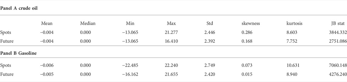
TABLE 1. Descriptive statistics of daily rate of return.

Table 1 shows that where the mean of the rate of return is less than zero, it indicates that both the crude oil price and the gasoline price are declining. Where the median of the rate of return is zero, it indicates that the number of days of rising prices and falling prices are roughly equal in the period of the sample. From the point of view of minimum, maximum, and standard deviation, the price of gasoline spots varies most, and the risk of fluctuations of the price of gasoline spots is the greatest. As for the daily rates of return on the four products, the skewness coefficients are all greater than zero, indicating a right shift in their distributions. The kurtosis coefficients are more than 3, indicating that the distributions of the rates of return on the four products are in “leptokurtosis and fat-tail”. The JB statistics further confirm that the distributions of the rates of return on the four products are significantly different from the normal distribution, so the risk measurement and risk management on the basis of normal distribution are inaccurate. The last column shows the correlation coefficient of the rates of return on crude oil futures and spots is 0.908, while the correlation coefficient of the rates of return on gasoline futures and spots is 0.836. A higher correlation coefficient indicates that the corresponding futures are better risk hedging tools for spot assets.

3.1 Risk measurement

First, by using the nonparametric method, we measure the risks of the two products in the whole samples, with the result noted as NPK-CVaR. Meanwhile, the measurement result of CVaR under normal distribution is given as Norm-CVaR for comparison. In addition, because values of CVaR are related to the level of confidence, a series of different confidence levels are taken to test the measurement results. The results are shown in Table 2.

TABLE 2

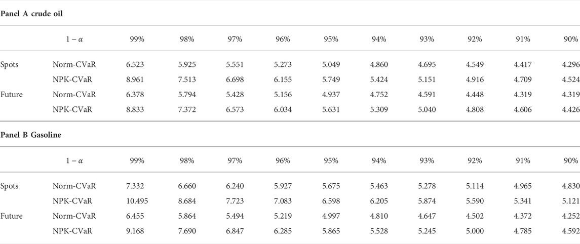
TABLE 2. Risk measurement under different confidence level.

Table 2 shows that with all the four products and confidence levels $1-\alpha$, Norm-CVaR is less than NPK-CVaR, indicating that the normal distribution assumption always underestimates the risk of energy spots and futures in reality. In addition, according to the comparison between spots risk and futures risk, the measurement results of crude oil and gasoline show that no matter under nonparametric estimation method or normal distribution assumption, the risk value of futures are greater than that of the corresponding spots.

To see the differences of risks measured by the two different methods more directly, we use kernel estimation method and normal distribution to fit the sample distribution of the rates of return on the four products (Figure 1). Specifically, based on the sample data of the rates of return on the four products, the density function of the real data is estimated through kernel estimation, and the image is noted as NPK. As a comparison, the normally distributed density function is used to fit the density function of the sample data. That is to say, supposing that the real data are in normal distribution, we estimate the mean and the standard deviation through sample data, and the normally distributed density function can be obtained and noted as Norm in the figure. It can be seen from the four figures that compared with the density function in normal distribution, density functions estimated by NPK have higher peaks and thicker left tail and right tail. This characteristic of “leptokurtosis and fat-tail” is vital for measurement and management of energy risk. For the long position (short position), the thicker left tail (right tail) indicates a greater probability of larger losses in the real energy market, which is seriously underestimated under normal distribution. This is consistent with the conclusion of Table 2; that is, the risk measurement under the normal distribution assumption tends to underestimate the risk.

FIGURE 1

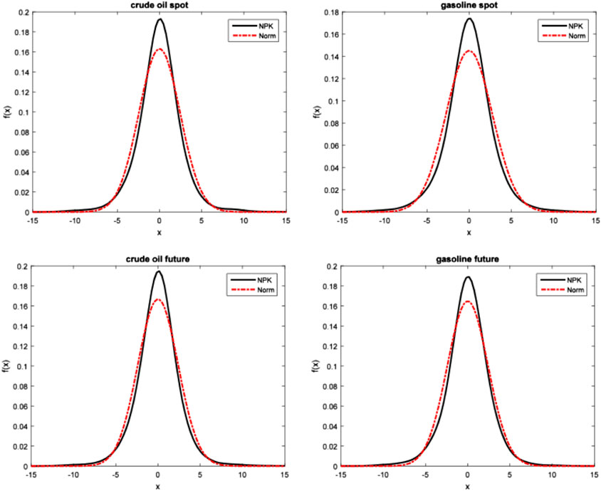
FIGURE 1. Sample distribution fitting of rates of return on futures and spots.

3.2 Risk hedging

This section uses the futures data and spots data of crude oil and gasoline to study the risk hedging based on CVaR. Specially, we use the futures of the crude oil and gasoline to hedge the risk of the corresponding spots. As a comparison, we present the hedging performance under the NPK CVaR and the Norm CVaR. The previous analysis has shown that the Norm CVaR tends to underestimate the actual risk, and CVaR can be expressed as a linear function of the mean and standard deviation under normal distribution assumption, while only taking into account the information on the first two order moments. When the financial market data are in non-normal distribution, investors will pay more attention to higher moments of market data in addition to the first two moments, such as mean and variance. Therefore, Cao et al. (2010) proposed a semi-parametric method to estimate CVaR. In fact, their method is the Cornish-Fisher expansion of CVaR (CFM CVaR), which includes the information on the third moment and fourth moment of the market data without any distribution assumption. This method is an improvement of normal method. Although CFM CVaR reflects the information on the first four moments of the risk factors, the information on higher order moments cannot be included because of the complexity of the formulas. The nonparametric kernel estimation method can get the sample distribution function of the market data exactly without any distribution setting, and therefore that the information on higher moments can be obtained. Theoretically, if the sample size is large enough, the nonparametric kernel estimation method can get the information on all moments of the risk factors. Therefore, we compare the performance of the three methods in the actual risk hedging. We consider both the static hedging strategy and the dynamic hedging strategy. Static hedging strategy, which is the optimal hedging strategy obtained from the training subsamples, is applied to the training subsamples and testing subsamples to test the in sample and out of sample performances of the hedging strategies.

It is a defect that the static hedging assumes that the distribution of the sample data in the sample interval is unchanged, while the actual financial market environment is constantly changing. Therefore, if the sample interval is too long and the distribution of rate of return changes, then there may be deviation in the static hedging. In dynamic hedging, long intervals are divided into several short intervals, in which the distribution of rates of return is assumed to be unchanged. This avoids the problem in static hedging that the distribution of the rates of return is unchanged in a long interval. However, the defect in dynamic hedging is that the position of the futures needs to be constantly adjusted, which increases the cost of risk hedging. The dynamic hedging strategy is constructed as follows: the optimal hedge ratio is obtained from the initial 1565 training subsamples, and is applied to the next 10 trading days (2 weeks). The training subsamples are then updated by replacing the oldest 10 samples by the data of the 10 trading days, as mentioned earlier, while the training sample size of 1565 is unchanged. The new hedge ratio is obtained from the updated training subsamples, and is applied to the next 10 trading days, and so on until to the end of the sample period. This method reflects the latest transaction information by dynamically adjusting the training subsamples. Finally, based on the dynamic hedge ratio, the sequence of the portfolio rate of return is obtained and the out of sample performance (e.g., mean, standard deviation and CVaR) are calculated, see Table 3.

TABLE 3

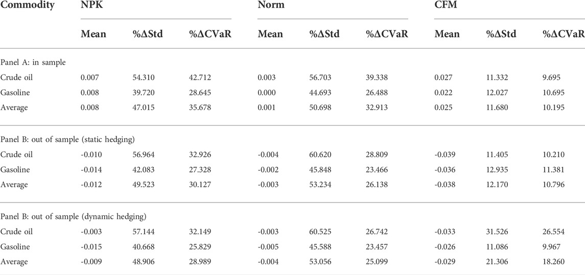
TABLE 3. Comparison of the hedging effect of the three methods.

Table 3 shows the mean, the decline in the standard deviation (%ΔStd), and the decline in the CVaR (%ΔCVaR) of the portfolio rate of return after hedging based on the three methods. After being hedged by three methods, the CVaR and the standard deviation declined greatly. This shows whether the decline in the CVaR is the largest based on NPK CVaR from the point of view of a single asset or an average value. Specifically, NPK CVaR is superior to Norm CVaR, and Norm CVaR is superior to CFM CVaR. This indicates that as a modification to Norm, semi-parametric CFM is not satisfactory in practice. The decline in the standard deviation is the greatest in the Norm CVaR method, mainly because CVaR is the linear function of the standard deviation in the Norm method, and to minimize Norm CVaR is to minimize the standard deviation. The standard deviation is a symmetric index. Its decline may be caused by the decline, either in the left tail or in the right tail of the distribution. This shows that the decline in the standard deviation in Norm method is larger than that in NPK method, which is largely due to the decline in the right tail in the table because the left decline of CVaR in Norm is smaller than that in NPK. Similarly, the sequence of standard deviation declines from large to small is in the sequence of Norm, NPK, and CFM. Finally, the conclusion by the mean is mixed. The means in the three methods after hedging are all positive in sample, while they are negative out of sample. This happens because the mean of the rate of return on spots before hedging is positive in sample, while it is negative out of sample.

From Figures 2–5, the histograms of the pre-hedging and post-hedging rates of return on the two energies in and out of samples are shown, respectively. Only the hedging image in NPK CVaR is given, because the risk decline in it is the largest. It can be seen directly from the figures that after hedging, the histograms are more concentrated, and the tail samples at both ends are less with most of the samples distributed on the right side of zero. This shows that hedging significantly reduces the risk in the left tail. The empirical results show that the NPK method that we proposed is more effective to measure the actual energy risk and carry out more effective risk hedging.

FIGURE 2

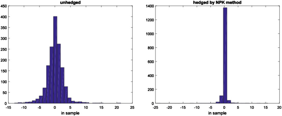
FIGURE 2. Histogram of crude oil (in sample).

FIGURE 3

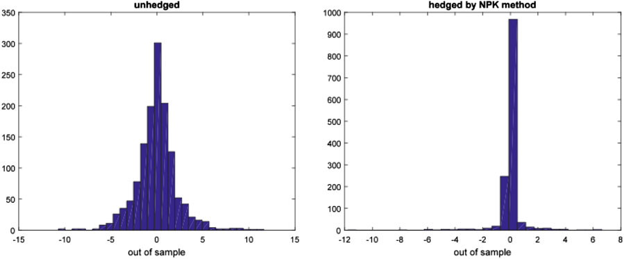
FIGURE 3. Histogram of crude oil (out of sample).

FIGURE 4

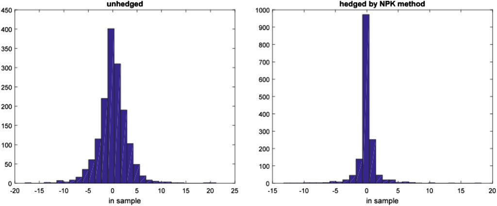
FIGURE 4. Histogram of gasoline (in sample).

FIGURE 5

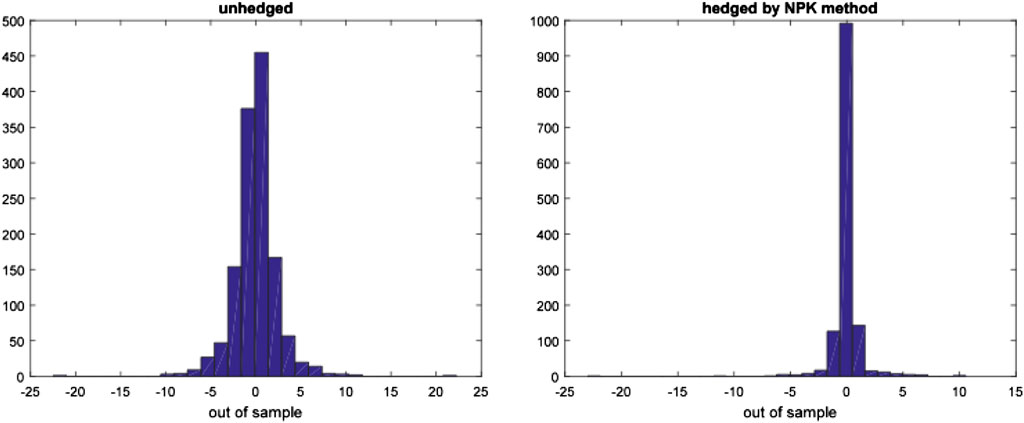
FIGURE 5. Histogram of gasoline (out of sample).

4 Conclusion

The accurate measurement of energy risk, and risk regulation and management have become important issues to be solved by academia and governments. However, VaR, which is the main tool for measuring risk, does not satisfy the subadditivity axiom and is defective in practical application. In this paper, we use a new nonparametric kernel estimation method to measure the price risk of energy. On this basis, we study how to hedge and manage the energy risk. Specifically, we use the CVaR to measure the downside risk of the energy, and obtain the NPK estimator of CVaR. Based on the estimation formula, we build the NPK CVaR risk hedging model and prove its convexity. The empirical results from crude oil and gasoline show that the NPK method that we propose is more effective to measure the actual energy risk and carry out more effective risk hedging.

Although CVaR is superior to VaR in nature, there are still some deficiencies in the practice of energy risk management and supervision. The effectiveness of CVaR depends on the accuracy of distribution tail estimation, but it is difficult to accurately estimate the tail of distribution. Under extreme market conditions, the original stable relationship between the influencing factors has been destroyed and the CVaR estimation may have a large deviation.

Data availability statement

The original contributions presented in the study are included in the article/supplementary material, and further inquiries can be directed to the corresponding author.

Author contributions

Conceptualization, LL; methodology, GH; software, GH; validation, GH and LL; formal analysis, GH; investigation LL; data curation, LL; writing—original draft preparation, LL; writing—review and editing, GH and LL; supervision, LL; funding acquisition, LL.

Funding

This paper is supported by the National Natural Science Foundation of China (No. 72003080), Southern Marine Science and Engineering Guangdong Laboratory (Zhuhai) (No. SML2021SP203), Carbon Emissions Accounting and Evaluation System of Marine Industry in Guangdong [No. GDNRC (2022)47] Doctor patient relationship model, form, governance, and conflict resolution in the context of big data (No. 299-gk19g051).

Conflict of interest

The authors declare that the research was conducted in the absence of any commercial or financial relationships that could be construed as a potential conflict of interest.

Publisher’s note

All claims expressed in this article are solely those of the authors and do not necessarily represent those of their affiliated organizations, or those of the publisher, the editors and the reviewers. Any product that may be evaluated in this article, or claim that may be made by its manufacturer, is not guaranteed or endorsed by the publisher.

References

Acerbi, C., and Tasche, D. (2002). On the coherence of expected shortfall. J. Bank. Finance 26, 1487–1503. doi:10.1016/S0378-4266(02)00283-2

CrossRef Full Text | Google Scholar

Alexander, G. J., and Baptista, A. M. (2004). A comparison of VaR and CVaR constraints on portfolio selection with the mean-variance model. Manag. Sci. 50 (9), 1261–1273. doi:10.1287/mnsc.1040.0201

CrossRef Full Text | Google Scholar

Aloui, C., and Mabrouk, S. (2010). Value-at-risk estimations of energy commodities via long-memory, asymmetry and fat-tailed garch models. Energy Policy 38 (5), 2326–2339. doi:10.1016/j.enpol.2009.12.020

CrossRef Full Text | Google Scholar

Angelidis, T., Benos, A., and Degiannakis, S. (2004). The use of GARCH models in VaR estimation. Statistical methodology Stat. Methodol. 1 (1–2), 105–128. doi:10.1016/j.stamet.2004.08.004

CrossRef Full Text | Google Scholar

Artzner, P., Delbaen, F., Eber, J., and Heath, D. (2010). Coherent measures of risk. Math. Finance 9 (3), 203–228. doi:10.1111/1467-9965.00068

CrossRef Full Text | Google Scholar

Artzner, P., Delbaen, F., Eber, J. M., and Heath, D. (1997). Thinking coherently. Risk 10 (11), 68–71.

Google Scholar

Cao, Z., Harris, R. D., and Shen, J. (2010). Hedging and value at risk: a semi-parametric approach. J. Fut. Mark. 30, 780–794. doi:10.1002/fut.20440

CrossRef Full Text | Google Scholar

Costello, A., Asem, E., and Gardner, E. (2008). Comparison of historically simulated var: evidence from oil prices. Energy Econ. 30 (5), 2154–2166. doi:10.1016/j.eneco.2008.01.011

CrossRef Full Text | Google Scholar

Degiannakis, S. (2004). Volatility forecasting: evidence from a fractional integrated asymmetric power arch skewed-t model. Appl. Financ. Econ. 14 (18), 1333–1342. doi:10.1080/0960310042000285794

CrossRef Full Text | Google Scholar

Duffie, D., and Pan, J. (1997). An overview of value at risk. J. Deriv. 4 (3), 7–49. doi:10.3905/jod.1997.407971

CrossRef Full Text | Google Scholar

Engle, R. F., and Manganelli, S. (2004). Caviar: conditional autoregressive value at risk by regression quantiles. J. Bus. Econ. Statistics 22 (4), 367–381. doi:10.1198/073500104000000370

CrossRef Full Text | Google Scholar

Fan, Y., Zhang, Y. J., Tsai, H. T., and Wei, Y. M. (2008). Estimating ‘value at risk’ of crude oil price and its spillover effect using the ged-garch approach. Energy Econ. 30 (6), 3156–3171. doi:10.1016/j.eneco.2008.04.002

CrossRef Full Text | Google Scholar

Hu, H., Wang, Y., Zeng, B., Zhang, J., and Shi, J. (2017). Cvar-based economic optimal dispatch of integrated energy system. Electr. Power Autom. Equip. 37 (6), 209–219. doi:10.16081/j.issn.1006-6047.2017.06.028

CrossRef Full Text | Google Scholar

Jinbo, H., Ding, A., Li, Y., and Lu, D. (2020). Increasing the risk management effectiveness from higher accuracy: A novel non-parametric method. Pacific Basin Finance J. 62, 101373. doi:10.1016/j.pacfin.2020.101373

CrossRef Full Text | Google Scholar

Jin, H. Y., Sun, H. B., Niu, T., Guo, Q. L., and Wang, B. (2019). Coordinated dispatch method of energy-extensive load and wind power risk constraints. Automation Electr. Power Syst. 43 (16), 9–18. doi:10.7500/AEPS20180901001

CrossRef Full Text | Google Scholar

Jorion, P. (2000). Value at risk: the new benchmark for managing financial risk. 2nd ed. New York, United States: McGraw-Hill.

Google Scholar

Kang, S. H., and Yoon, S. M. (2007). Long memory properties in return and volatility: evidence from the korean stock market. Phys. A Stat. Mech. its Appl. 385 (2), 591–600. doi:10.1016/j.physa.2007.07.051

CrossRef Full Text | Google Scholar

Krehbiel, T., and Adkins, L. C. (2015). Price risk in the nymex energy complex: an extreme value approach. J. Fut. Mark. 25 (4), 309–337. doi:10.1002/fut.20150

CrossRef Full Text | Google Scholar

Li, Q., and Racine, J. S. (2007). Nonparametric econometrics: theory and practice. New Jersey, United States: Princeton University Press.

Google Scholar

Marimoutou, V., Raggad, B., and Trabelsi, A. (2009). Extreme value theory and value at risk: application to oil market. Energy Econ. 31 (4), 519–530. doi:10.1016/j.eneco.2009.02.005

CrossRef Full Text | Google Scholar

Markowitz, H. (1952). Portfolio selection. J. Finance 7 (1), 77–91. doi:10.1111/j.1540-6261.1952.tb01525.x

CrossRef Full Text | Google Scholar

Mcneil, A. J., and Frey, R. (2000). Estimation of tail-related risk measures for heteroscedastic financial time series: an extreme value approach. J. Empir. Finance 7 (3), 271–300. doi:10.1016/S0927-5398(00)00012-8

CrossRef Full Text | Google Scholar

Muñoz, J. I., Nieta, A. A. S. D. L., Contreras, J., and Bernal-Agustín, J. L. (2009). Optimal investment portfolio in renewable energy: the spanish case. Energy Policy 37 (12), 5273–5284. doi:10.1016/j.enpol.2009.07.050

CrossRef Full Text | Google Scholar

Rockafellar, R. T., and Uryasev, S. (2000). Optimization of conditional value-at-risk. Journal of risk 2, 21–42. doi:10.21314/JOR.2000.038

CrossRef Full Text | Google Scholar

Sadeghi, M., and Shavvalpour, S. (2006). Energy risk management and value at risk modeling. Energy Policy 34 (18), 3367–3373. doi:10.1016/j.enpol.2005.07.004

CrossRef Full Text | Google Scholar

Tang, T. L., and Shieh, S. J. (2006). Long memory in stock index futures markets: a value-at-risk approach. Phys. A Stat. Mech. its Appl. 366 (1), 437–448. doi:10.1016/j.physa.2005.10.017

CrossRef Full Text | Google Scholar

Vithayasrichareon, P., and Macgill, I. F. (2013). Assessing the value of wind generation in future carbon constrained electricity industries. Energy Policy 53 (1), 400–412. doi:10.1016/j.enpol.2012.11.002

CrossRef Full Text | Google Scholar

Vithayasrichareon, P., and Macgill, I. F. (2012). Portfolio assessments for future generation investment in newly industrializing countries – a case study of Thailand. Energy 44 (1), 1044–1058. doi:10.1016/j.energy.2012.04.042

CrossRef Full Text | Google Scholar

Wu, G., Wei, Y. M., Fan, Y., and Liu, L. C. (2007). An empirical analysis of the risk of crude oil imports in China using improved portfolio approach. Energy Policy 35 (8), 4190–4199. doi:10.1016/j.enpol.2007.02.009

CrossRef Full Text | Google Scholar

Yao, H. X., Li, Z. F., and Lai, Y. Z. (2013). Mean–CVaR portfolio selection: a nonparametric estimation framework. Comput. Operations Res. 40 (4), 1014–1022. doi:10.1016/j.cor.2012.11.007

CrossRef Full Text | Google Scholar

Youssef, M., Belkacem, L., and Mokni, K. (2015). Value-at-risk estimation of energy commodities: a long-memory garch–evt approach. Energy Econ. 51, 99–110. doi:10.1016/j.eneco.2015.06.010

CrossRef Full Text | Google Scholar

Zhang, Y., Wang, J., Ding, T., and Wang, X. (2018). Conditional value at risk-based stochastic unit commitment considering the uncertainty of wind power generation. IET Gener. Transm. &amp. Distrib. 12 (2), 482–489. doi:10.1049/iet-gtd.2017.0509

CrossRef Full Text | Google Scholar