Correlations Between Wake Phenomena and Fatigue Loads Within Large Wind Farms: A Large-Eddy Simulation Study

This work proposes a methodology aiming at simulating the whole wind farm behavior, from the wake phenomena to the wind turbine fatigue loads, in a both accurate and efficient way and for a large range of operating conditions. This approach is based on Large Eddy Simulation (LES), coupled to an Actuator Disk (AD) approach. In order to recover pertinent fatigue loads with that wind turbine model, the blade trajectories are replicated through the disk and the AD aerodynamic forces are interpolated onto these “virtual blades” at each time step. The wake centerline is also tracked in the whole wind farm, in order to highlight the correlations between the wake phenomena and the wind turbine fatigue damage. The described methodology is deployed in simulations of the Horns Rev wind farm for several wind directions. The time-averaged power production is first compared to measurements and other LES results, with a very good agreement for large wind sectors. We then investigate the fatigue loads for several machines inside the wind farm and wind directions. We clearly show the link between the upstream wake movement and the resulting high and low frequency oscillations of the root bending moments and of the yaw and tilt moments, and therefore on the resulting fatigue equivalent loads. This study demonstrates the capacity of the numerical tool to accurately capture the wind farm flow and the rotor behaviors, as well as the correlations between the wake phenomena and the resulting fatigue loads.

1 Introduction

Fatigue is a critical factor in the lifetime of a wind turbine and is one of the causes of failure of the machine components (Sheng, 2013). The actual loads that contribute to fatigue of a wind turbine originate from a variety of sources: high winds, wind shear, gravity and/or potential yaw errors, turbulent fluctuations, ambient gusts, starts and stops of the machine, etc. Moreover, in a wind farm arrangement, fatigue phenomenon is exacerbated by the presence of other rotors: the wind turbines impacted by the wakes of the upstream machines see their cumulated fatigue damage rise due to the increase level of ambient turbulence and the wake meandering phenomenon. Wake effects are very complex and difficult to predict and they further increase the uncertainties in the predicted fatigue damage, leading to unexpected failures forsome wind turbine components. For some wind turbine subassemblies,the downtime associated with repair may be significant, mainly in the offshore environment: this decreases the wind turbine reliability, directly impacting the Levelized Cost of Energy, as demonstrated in Dao et al. (2019).

It is thus of a crucial importance to deploy efforts in the comprehension of the wake phenomena within a wind farm, and of their correlations with the resulting wind turbine fatigue damage, either to optimally design the wind farm, or to develop load alleviation strategies that can be used during its operation (Bossanyi, 2018; Kanev et al., 2018; Capello et al., 2020). This requires access to some recordings of fatigue load measurements, but also to the knowledge of the ambient flow field around of the machines. Information about fatigue loads can be recovered thanks to the SCADA data (Cosack, 2010; Vera-Tudela and Kühn, 2017; Movsessian et al., 2020) and additional sensors located at strategic locations on the machine (Larsen et al., 2013; Hansen et al., 2014; Herges, 2018), while met masts, sodar, or Lidar technology can help in visualising the ambient flow field, and the wake phenomenon in particular (Trujillo et al., 2011; Herges, 2018; Gao et al., 2019; Simley et al., 2021). For example, two wind turbines of the Scaled Wind Farm Technology (SWiFT) facility were highly instrumented (Naughton, 2017; Herges, 2018), with, among others, sensors at the blade roots in order to recover information of flapwise and edgewise moments. A DTU SpinnerLidar (Naughton, 2017) was also mounted on one wind turbine nacelle, giving measurements of the downstream wake velocity field. Two wind turbines of the seven machines of the La Sole du Moulin-Vieux wind farm were also instrumented with additional sensors, in the context of the SMARTEOLE project (Simley et al., 2021; Hegazy et al., 2022). Several lidars and sodar were also added, in order to recover information of the wake behavior (Simley et al., 2021). These instrumented wind farms were mainly used to test control strategies aiming at increasing the power production (induction control and/or wake steering), but the impacts of the control actions on the lifetime of the wind turbines were also investigated. However, most of the wind turbines in operation are not fully instrumented, and if they are, this is often for a few machines inside the wind farm (Larsen et al., 2013; Hansen et al., 2014) or the access to those data is often limited. Moreover, when Lidars are installed on a wind farm site, there are often only one or two of them, giving access to the velocity field around a very small number of wind turbines. If we want investigate the wake phenomena and their impacts on the wind turbine damage in the whole wind farm, another strategy has to be considered.

Numerical studies offer a convenient framework to perform investigations of the fatigue loads for rotors in a wind farm arrangement, as they give access to pertinent information about the blade loading fluctuations and also provide the wind flow in the whole wind farm. They can also be used as a virtual laboratory in order to elaborate and test global control schemes. As more and more efforts are made in order to use information coming from wind turbine loads for estimating relevant characteristics of the environment (Bottasso et al., 2018) or for predicting the wake characteristics downstream of the machines (Aubrun et al., 2015; Muller et al., 2015; Lejeune et al., 2020), which could be used in the control strategies, it is important that those numerical environments accurately capture the blade loads.

Several numerical methods that capture fatigue loads at a wind farm scale exist, and their use depends on the considered application. Lower fidelity approaches, usually implying a Blade Element Momentum (BEM) method combined to a wake model, are often used to evaluate the fatigue loads for the lifetime of the wind farm. Indeed, their low computational costs allow simulations that cover all the incoming wind speeds and directions that a wind farm will meet during its operation. The BEM approach has already demonstrated its performances to accurately represent the wind turbine behavior, even immersed in a complex turbulent inflow (Bangga and Lutz, 2021), and its coupling to an aero elastic code allows to perform accurate fatigue load investigations at the scale of one wind turbine (Damiani et al., 2018; Madsen et al., 2020). Due to its good performances and low computational costs, this approach is widely used in the industry, and many research works still investigate how to further improve this method (Bangga and Lutz, 2021; Jin and Yang, 2021; Potentier et al., 2021). Its combination to wake models that capture the unsteady wake behavior while remaining computationally inexpensive, allows to extend the studies at the scale of a wind farm. For example, Larsen et al. (2013) validated a numerical approach based on a Dynamic Wake Meandering (DWM) model (Larsen et al., 2007) and a BEM implemented in the aeroelastic code HAWC2, by comparing the fatigue loads of one turbine within the Egmond aan Zee wind farm to actual measurements. Galinos et al. (2016) used the same method for computing the representative 20-years lifetime fatigue loads and power production for the Horns Rev wind farm. Schmidt et al. (2011) also investigated the fatigue loads for one machine inside the Horns Rev wind farm, using the DWM implemented into GH Bladed. Those fast approaches or variants of them were also used to investigate control strategies that account for fatigue loads (Harrison et al., 2020; van Dijk et al., 2017; Riva et al., 2020; Stanley et al., 2020). Efforts have also been made to develop operational wake models of higher fidelity (Lejeune et al., 2020). Thanks to their efficiency, the approaches described above are also particularly suitable for model based control, allowing the prediction of the wind turbine fatigue loads and wake behavior and a more accurate control.

Although the DWM model used in several of these approaches account for the wake meandering, it remains of medium fidelity and it cannot capture all the fine physics arising of the complex wake flow phenomena (e.g., wake merging or wake destructuration). If we want to have a high fidelity virtual environment in which we can study fatigue loads in more detail, test the global control strategies, or verify/validate the low and medium fidelity approaches described above, we have to increase the accuracy of the numerical tool. Numerical approaches with a fully resolved wind turbine (Kim et al., 2016; Bangga and Lutz, 2021) are affordable at the scale of one rotor. Large eddy simulation (LES) coupled to a wind turbine model is currently one of the most appropriate approaches for an accurate and efficient representation of a wind farm. Indeed, LES intrinsically and accurately captures unsteady effects and thus the complex wake phenomena that contribute for a significant part of the fatigue damage. For example, LES, coupled with an Actuator Line (AL) approach for the wind turbine model, was used in several numerical studies for investigating fatigue loads and damages. Lee et al. (2018) investigated fatigue loads for two floating wind turbines, with the second machine located in the wake of the first one. The flow solver was two-way coupled with the aeroelastic code FAST (Jonkman and Buhl, 2005). Liu et al. (2020) also considered fatigue damages for a tandem of wind turbines, but the AL method was only adopted for the first wind turbine, in order to simulate the wake flow field numerically. The fatigue loads of the downstream rotor were thus computed using an aeroelastic tool coupled to a Blade Element Momentum (BEM) method. Meng et al. (2020) studied the fatigue damages through a small wind farm with nine wind turbines, modelled using an aeroelastic AL method. Churchfield et al. (2015) performed LES of 36 wind turbines in order to compare the fatigue loads of some machines to those obtained using the DWM model coupled to FAST (Jonkman and Buhl, 2005) and those available from measurements.

The above, non-exhaustive, literature overview shows that most of LES studies considered a limited number of rotors, or a limited number of simulation cases (Churchfield et al., 2015), as the AL method requires fine spatio-temporal resolutions. However, the complexity of the wake flow phenomena and of their correlations with the wind turbine damage increases as we consider larger wind farms or several wind conditions. It is therefore crucial that the numerical studies also involve a larger number of wind turbines and operating conditions. This imposes a coarsening of the resolution, in order to keep the computation cost acceptable. The use of an Actuator Disk (AD) approach for modelling the rotor behavior thus appears as the most relevant procedure: with this model, the actual geometry of rotor blades is replaced by a regularized body force term acting over the surface swept by the blades. The most advanced AD approaches include torque effects and force computations based on the prevailing velocities at the disk location (Martínez-Tossas and Leonardi, 2013; Wu and Porté-Agel, 2015; Moens et al., 2018). This last feature allows the wind turbine model to capture temporal and spatial rotor loads variations, which could give relevant information about blade loading and bending moments. In order to reproduce pertinent blade loads, a possible approach consists in replicating the blade trajectories through the disk and interpolate the AD aerodynamic forces onto these “virtual blades” at each time step. It is thus possible to integrate the aerodynamic forces along the blades, and to easily recover fatigue loads, as in a discrete line type approach. Moens et al. (Forthcoming 2022b) used this methodology and showed that an AD model at a coarse resolution, typical of that used in wind farm simulations, gave fatigue loads and damages that were in excellent agreement with those obtained using a Vortex Particle-Mesh method coupled to immersed Lifting Lines (Chatelain et al., 2017; Caprace et al., 2020) at a finer resolution.

We here propose to use LES coupled to an AD model in order to investigate the fatigue damages in a large wind farm and their variations according to the incoming wind direction and the position of the wind turbine. Our objective is to demonstrate that such a numerical tool is appropriate for accurately simulating both wakes and wind turbine behaviors, and thus offers a suitable virtual environment for investigating load alleviation strategies or further understanding correlations between wake phenomena and fatigue loads at a wind farm scale. We consider the Horns Rev wind farm, a Danish offshore wind farm, for which power measurements were available and treated in several research works and papers (Barthelmie et al., 2007; Barthelmie et al., 2009; Barthelmie et al., 2010; Barthelmie et al., 2011). This will allow us to verify the performances of the code in terms of power prediction, before investigating the fatigue loads. We also track the wake centerline position downstream of each machine, based on a technique detailed in Coudou et al. (2018) in order to highlight the correlations between the large scale movement of the wake (i.e., the wake meandering) and the fatigue loads on a rotor impacted by this wake.

The flow solver, the wind turbine model and the methods for recovering the AD fatigue loads and tracking the wake center are described in Section 2. Section 3 reports the configuration of the Horns Rev wind farm, as well as the several wind directions that are investigated in this work. Section 4 present the main results of this work, which are: 1) the comparison of the power production with measurements available in Barthelmie et al. (2009) and other LES performed by Wu and Porté-Agel (2015), 2) the correlations between the wake movement and the instantaneous fatigue loads for several machines and incoming wind directions, and 3) the resulting load cycle distribution and fatigue damages inside the wind farm. Our conclusions are finally drawn in Section 5.

2 Methods

2.1 Flow Solver

We consider the Large Eddy Simulation (LES) of incompressible flows. It is performed using an in-house developed fourth-order finite differences code (Duponcheel et al., 2008; Duponcheel et al., 2014), formulated in primitive variables (i.e. in velocity and pressure) and using a staggered mesh arrangement. Using a Cartesian coordinate system, the Navier-Stokes equations (supplemented by a subgrid scale (SGS) model) are formulated as

$\frac{\partial u_i}{\partial x_i}=0,(1)$

$\frac{\partial u_i}{\partial t}+u_j\frac{\partial u_i}{\partial x_j}=-\frac{1}{\rho }\frac{\partial p}{\partial x_i}+\nu \frac{{\partial }^2{u}_i}{\partial x_j\partial x_j}+\frac{\partial {\tau }_{ij}^M}{\partial x_j}+\frac{f_i}{\rho },(2)$

where $i,j\in \left(\mathrm{1,2,3}\right)$ correspond to the streamwise (x, u), vertical (y, v) and lateral (z, w) directions and velocity components, respectively; p is the pressure and f_i is the external body force (per unit volume) acting on the flow to model the wind turbine (discussed in Section 2.3); ρ and ν are the fluid density and molecular viscosity, respectively; ${\tau }_{ij}^M$ is the SGS stress tensor model. We here use a classical Smagorinsky model (Smagorinsky, 1963).

The equations were initially discretized in space using the fourth-order finite differences scheme of Vasilyev (2000), which is such that the discretized convective term conserves the kinetic energy on Cartesian meshes. Recent developments saw the addition of wall modeling strategies. This required the convective term to be rewritten; this new version thus preserves the discrete kinetic energy up to fourth order (in the absence of wall modeling procedure, see Thiry (2017) for details) and it conserves the momentum exactly on uniform grids. In this work, only the new version of the code is used as we consider simulations of rotors in an atmospheric boundary layer.

Equations 1 and 2 are solved using a fractional-step method with the “delta” form for the pressure (Lee et al., 2001). The Poisson equation for the pressure is solved using a multigrid solver with a Gauss-Seidel smoother. The time integration is carried using a second-order Adams-Bashforth scheme.

2.2 Generation of the Atmospheric Turbulence

There are two main approaches for generating turbulent inflows in LES. The first one implies using synthetic turbulence field generation techniques, while the second one consists in generating turbulence using a precursor LES.

In the first approach, the synthetic turbulence field is pre-generated from a chosen model and is then imposed over a mean profile at the inlet of the simulation of interest (here denoted the wind farm (WF) simulation). The main advantage of this method is the low computational cost overhead compared to the WF simulation. The most advanced models match physical spectra and moments that are assumed to evolve rapidly enough into realistic turbulence, such as that developed by Mann (1998) and widely used in the wind energy domain. However, Munters et al. (2016) demonstrated that the adaptation length required for the larger structures to develop inside the WF simulation was very important. Those large turbulent structures are known to contribute to the wake meandering process (Espana et al., 2011) and are thus particularly important to capture. This large establishment length sensibly increases the computational domain and thus the computational costs. Consequently, the second approach is used in the present work, i.e. generating the turbulent inflows using a precursor LES.

The precursor technique relies on an auxiliary wind flow simulation, performed on an independent domain without wind turbines, for generating turbulent inflow conditions. This auxiliary simulation is here denoted the Atmospheric Boundary Layer (ABL) simulation. When it reaches a statistically-steady state, either yz-planes of instantaneous velocities are saved to generate an independent data base inflow data, or this auxiliary simulation runs concurrently with the WF simulation (concurrent simulations), which allows inflow conditions to be directly transferred to the inlet of the main domain. The use of precursor techniques has increased in wind energy in recent years (Wu and Porté-Agel, 2015; Munters et al., 2016), and is strongly recommended for wind farm simulations, in order to obtain faithful flow structures impacting the wind turbines (Park et al., 2014).

In this work, concurrent simulations are considered, in order to avoid saving a large amount of inflow velocity planes. For the ABL simulation, periodic conditions are enforced in the horizontal directions, while a no-through flow is imposed at the top. At the bottom, a wall stress model (Thiry, 2017) for a rough wall is applied, to compute the surface shear stress as a function of the LES velocity field at the third vertical grid point and a roughness length, y₀. The flow is driven by a pressure gradient that is continuously adapted in order to conserve an imposed mass flow, itself preliminary determined to achieve the desired hub velocity and turbulence intensity (TI). For the WF simulation, outflow conditions are then imposed at the outlet boundary, while periodic conditions are kept in the spanwise direction. Again, a wall model and a no-through flow condition are imposed at the bottom and top, respectively. The code allows different resolutions and streamwise domain sizes for the ABL and the WF simulations.

In the present work, thermal and stratification effects are not included; the resulting simulations are thus equivalent to truly neutral atmospheric boundary layer (ABL) cases.

2.3 Wind Turbine Modelling

The wind turbine model targets the context of accurate and still affordable LES of wind farms, we thus choose a rotating Actuator Disk (AD), discretized in the radial and tangential directions, and for which the aerodynamic forces are estimated from local velocities. The AD method is here improved with a tip-loss factor: this correction is based on the commonly used Glauert tip-loss factor, for which the infinite upstream velocity is estimated based on the 1D momentum theory, applied on each AD elements (Moens et al., 2018). The AD forces are finally translated into bulk forces for the LES equations (f_i in Eq. 2) by using a second-order mollifier, the M₄ kernel (Monaghan, 1985). This AD approach, supplemented with the tip-loss factor, has been verified with a higher fidelity approach in a finer resolution, a Vortex Particle-Mesh method coupled to immersed lifting lines (Chatelain et al., 2017; Caprace et al., 2020): we refer to Moens et al. (2018) for the comparison results and additional methodological details.

2.4 Estimation of Fatigue Loads

In the present work, we will investigate four different moments: the blade flapwise and edgewise root bending moments and the rotor yaw and tilt moments. They are evaluated based on the aerodynamic contributions only. The flapwise and edgewise moments on blade b are denoted M_f,b and M_e,b, respectively, and are evaluated as

$M_{f,b}={\int }_{R_{hub}}^{R_{tip}}\left(r-R_{hub}\right){\mathbf{F}}_{\mathbf{b}}.{\mathbf{e}}_{\mathbf{n}}dr,(3)$

$M_{e,b}={\int }_{R_{hub}}^{R_{tip}}r{\mathbf{F}}_{\mathbf{b}}.{\mathbf{e}}_{\theta }dr,(4)$

where F_b is the aerodynamic blade force per length; e_n and e_θ are the unit vectors normal and tangential to the rotor plane, respectively; R_hub and R_tip are the radii at the hub and the tip locations. The yawing and the tilting moments, denoted M_y and M_t, respectively, are expressed as

$M_y=\sum _{b=1}^{N_b}{\mathbf{e}}_{\mathbf{y}}.{\int }_{R_{hub}}^{R_{tip}}{\mathbf{x}\times \mathbf{F}}_{\mathbf{b}}dr,(5)$

$M_t=\sum _{b=1}^{N_b}{\mathbf{e}}_{\mathbf{z}}.{\int }_{R_{hub}}^{R_{tip}}{\mathbf{x}\times \mathbf{F}}_{\mathbf{b}}dr,(6)$

where N_b is the number of blades; x is the position from the hub center and the considered force point; e_y and e_z correspond the yaw and tilt axes, respectively. The present study assumes that only the normal force component contributes to the yaw and tilt moments. Indeed, as mentioned above, the moments are calculated based on the aerodynamic contributions only. For the wind conditions considered in this work, the tangential forces will be roughly 10 times lower than the normal forces. Their contribution to M_y and M_t is thus expected to be less important than that related to the normal forces. This is also reinforced by the fact that the tangential forces are multiplied by the shaft length or a fraction of the shaft length in the M_y or M_t calculations (if we consider investigating the fatigue damage on the main shaft). This shaft length is usually small. In comparison, the normal forces are multiplied by the local radius, which is higher than the shaft length for the large part of the blade. If the gravitational loads are added in the computation of M_y and M_t, the contribution of the tangential forces might be no more negligible. However, for a well-balanced rotor, the contribution of the three blades cancels the effect of the gravity on the yawing moment. The gravitational loads play a role on the mean value of the tilting moment, and would add an offset in the temporal signal presented in this paper. As we only account for the cycle amplitudes in the equivalent moments (see Section 4.4), the addition of the gravity should not impact the fatigue analysis of the tilting moment.

For discrete line type approaches, the instantaneous blade loading is directly available and can be integrated along the blade span. For the AD method, we propose to replicate the blade trajectories through the disk and recompute blade-attached aerodynamic forces. At each particular radial position, r, and time, t, the forces F_b acting on the blade b are thus interpolated from the disk forces of the two adjacent disk elements at the same radius r. The instantaneous blade loading is directly available and can be integrated along the blade span to estimate the root bending moments. This procedure can be performed when the simulation is running, in order to avoid the save of a large amount of AD data and additional post-processing computations. Details about the procedure can be found in Moens et al. (Forthcoming 2022b), where it was shown that the fatigue loads estimated using this methodology were in excellent agreement with those obtained using a Vortex Particle-Mesh method coupled to immersed Lifting Lines (Chatelain et al., 2017; Caprace et al., 2020). This methodology has also been used in Moens et al. (Forthcoming 2022a), in order to investigate the individual pitch control within an AD framework, and again, the AD method provides blade moments that are really close to those obtained using a discrete blade type approach. This clearly positions the proposed approach as an efficient method for recovering pertinent and accurate information about fatigue loads.

The simulation tool is not coupled to an aeroelastic code, and the blades thus act as rigid bodies.

2.5 Wake Centerline Tracking

We choose the most robust technique of Coudou et al. (2018) to perform tracking of the wake centroid, (y_c, z_c), in cross-flow planes located downstream of a wind turbine. It is based on finding the minimum of a convolution product

$\left(y_c,z_c\right)=\mathrm{arg\; min}\left(p\left(y,z\right)*f_G\left(y,z\right)\right)(7)$

between the available power density in the flow

$p\left(y,z\right)=\frac{1}{2}u|\mathbf{u}{|}^2(8)$

and a Gaussian masking function

$f_G\left(y,z\right)=A\mathrm{e}\mathrm{x}\mathrm{p}\left(-\left(\frac{{\left(y-{\mu }_y\right)}^2}{2{\sigma }_y^2}+\frac{{\left(z-{\mu }_z\right)}^2}{2{\sigma }_z^2}\right)\right)(9)$

with A = 1, μ_y,z is equal to the wind turbine center, and σ_y and σ_z are set to 0.25D and 0.5D, respectively. Physically, this convolution method relies on the computation of the wind power inside a disk (with a Gaussian weighting) located in a cross-flow plane and with a diameter equal to the rotor diameter D. This disk center position can be shifted in the y − and z − directions; the wake center corresponds to the disk position for which the available power is minimum (Vollmer et al., 2016). Finally, by tracking the wake centroid in several downwind cross-flow planes, the wake centerline can be obtained.

For the wind farm simulations, the time-averaged freestream velocity profile is substracted from the velocity field before computing the convolution.

3 The Horns Rev Wind Farm

We leverage the above-described methodology toward the investigation of the fatigue loads for rotors inside a very large wind farm, and their variations according to the wind turbine location and the incoming wind direction. We also propose to correlate the rotor fatigue damage to the meandering of the upstream wakes.

We here consider the Horns Rev wind farm, an operational large offshore wind farm located 14 km away from the west coast of Denmark. The wind farm has a rated capacity of 160 MW; it comprises 80 Vestas v80 wind turbines arranged in a regular array of 8 by 10 turbines, as shown in Figure 1. The Vestas machine, characterized by a rated power of 2MW, has a rotor diameter equal to 80 m and a hub located at a height of 70 m. It is a variable speed machine, regulated with pitch and torque control schemes. The wind turbine modelization is not the main subject of this study, and its geometry, aerodynamics and controller are defined in Supplementary Appendix 1.

FIGURE 1

FIGURE 1. Horns Rev: Rotor organisation and definition of the main wind directions.

We perform simulations for nine wind directions α_w, performed each 2° from 262 to 278° (see Figure 1 for the definition of the wind direction); 270° corresponds to a “fully” westerly wind, where the turbine spacing is at its minimum, and the rotors in a line are perfectly aligned. We base our set-up on a measurement campaign presented in Barthelmie et al. (2009). In that study, measurements of power losses inside the Horns Rev wind farm were investigated and compared to results obtained with wake models. The presented cases included data for wind speeds equal to about 8 m/s and an ambient turbulence intensity below 8% in near neutral stability for the atmospheric boundary layer conditions. Using the same wind conditions and wind directions will allow us to compare our simulated power losses to measurements and verify/validate the code before investigating the fatigue loads.

For the present study, we only consider one ABL simulation that is used for the several wind directions. For each considered α_w, the wind flow in the WF simulation is always perpendicular to the inflow plane, so only the wind farm layout will vary for simulating the change in the incoming wind direction (this will be highlighted in the results below).

WF simulation The WF simulation extends over to L_x × L_y × L_z = 124.8D × 12D × 124.8D, leading to horizontal lengths of 9,984 m and a height of 960 m. This height is close to that of similar simulations performed for this wind farm (Wu and Porté-Agel, 2015; Munters et al., 2016). The horizontal lengths are set to be large enough to avoid an effect of the boundaries on the flow velocities at the wind farm level (this has been verified for simulations in coarse resolutions, not shown here), and to include all the investigated wind farm layouts. For this work, the resolution is set to about 12 points per rotor diameter in the transverse directions. This results from a compromise between accuracy and efficiency. The mesh is refined in the y-direction, from the ground to a height slightly above the highest point of the disk, in order to have a few points between the lowest disk position and the height where the velocity is sampled for the wall modelling procedure. The final mesh is a N_x × N_y × N_z = 1,536 × 128 × 1,536 grid that is uniform in the wall-parallel directions (Δx = Δz = 6.5 m) and that is partially stretched in the vertical direction. This stretching leads to uniform vertical grid below 150 m, with Δy_min = 3.75 m. Above that, Δy increases, to reach Δy_max ≃ 20 m at the top of the domain.

The time step is fixed to Δt = 0.125 s. The simulation time reaches about 1 hour for each simulated wind direction, and the flow statistics are computed during the last 40 min. For all wind directions, the first wind turbine is located 30 rotor diameters from the inlet and the wind farm is globally centered in the middle of the domain.

ABL simulation For the ABL simulation, the pressure gradient that drives the flow is adapted in order to conserve the desired hub velocity of 8 m/s and the TI of 8%. The domain size of the ABL simulation is equal to that used for the WF simulation, but the resolution is slightly decreased in the streamwise direction in order to save computational costs (from 1,536 points to 1,280 points). This leads to a N_x × N_y × N_z = 1,280 × 128 × 1,536 grid. Again, the mesh is uniform in the wall parallel directions (Δx and Δz are constant, and equal to 6.5 and 7.8 m, respectively) while the vertical direction is stretched according to the same procedure as that used for the WF simulation. The time step is the same as that defined in the WF simulation, i.e. Δt = 0.125 s.

The resulting time- and space-averaged velocity profile of the ABL simulation is presented in Figures 2A,B, and compared to the logarithmic law. u_τ is the roughness velocity, computed as the time- and space-averaged value of the simulation, and is equal to 0.292 m/s. The resulting TI_u (based on the streamwise component) and TI (based on the three velocity components) are also presented in Figure 2C; they are normalized by the unperturbed time-averaged velocity at hub height. We see that the ABL simulation captures the logarithmic law well, and leads to a mean streamwise velocity of 8 m/s at the hub height (see horizontal dashed-line in Figure 2A); this velocity is denoted ${\bar{U}}_{hub}$ The turbulence intensity is equal to 6.3 and 8.5%, for TI and TI_u, respectively, which is close to the expected conditions for the Horns Rev wind farm. We report these two values, as we cannot certify that the TI value given in Barthelmie et al. (2009) is computed based on the three velocity components, or based on the streamwise one only.

FIGURE 2

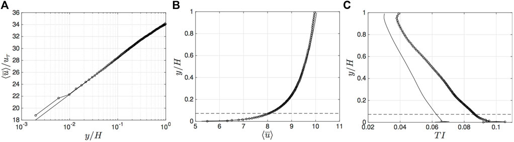
FIGURE 2. Time- and horizontally-averaged streamwise velocity profile (presented in both (A) and (B) but in different ways) and turbulence statistics (C) for the ABL simulation. In (A,B), the ABL velocity profile (solid line with circles) is compared to the logarithmic law (solid line). In (C), the TI is shown for statistics computed based on the streamwise component (solid line with circles) and based on the three velocity components (solid line). The horizontal dashed line represents the hub height and H is the height of the domain.

In order to give visual examples of the evolution and the complexity of the wind flow according to the incoming wind direction and the rotor position within the wind farm, we report on Figure 3 horizontal slices at hub height of instantaneous streamwise velocities for two particular wind directions, α_w = 262° and α_w = 270°. These two particular wind directions, as well as the resulting wake phenomena, will be discussed in more details in Section 4.2, where we will correlate the root bending moments and the yaw and tilt moments to the incoming flow.

FIGURE 3

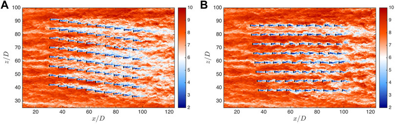
FIGURE 3. Instantaneous streamwise velocity on a horizontal plane at hub height for the wind directions α_w = 262° (A) and α_w = 270° (B). The units are in m/s.

4 Results

4.1 Comparisons of the Power Production With Measurements and Other Large Eddy Simulation Results

In order to verify the performances of the code for simulating large wind farms, we first compare the time-averaged power output of the present results to available observations in the reference paper of Barthelmie et al. (2009). The results are moreover compared to an other set of LES performed by Wu and Porté-Agel (2015). The Horns Rev measurements, the different LES, as well as the considered size of wind sectors, are detailed in the next paragraphs.

4.1.1 Comparison With Measurements

We first compare the present results with the observations of Barthelmie et al. (2009) (see Figure 4). For the measurements, the results are shown for several wind sectors, i.e., 270 ± 1°, ±5°, ±10°. When an observation with a reference time period of 10 min had the correct mean wind speed and TI, and a wind direction within the considered wind sector, it was selected for the analysis. We assume¹

1

It is not well detailed in Barthelmie et al. (2009).

that, for one observation, the power output of each rotor in a line is normalized to the power output of the first turbine in the same line. Each rotor power is then averaged on the selected number of observations. The power of each row was then computed as an average of the eight lines. We note that the amount of observations per wind sector is not mentioned in Barthelmie et al. (2009) and values of uncertainties or standard deviations are not available. Only the power output for the first eight rows were shown in the reference paper.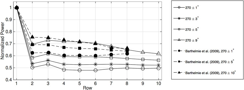

FIGURE 4

FIGURE 4. Comparison of the normalized mean power output data obtained from the measurements Barthelmie et al. (2009) and the present simulations, for several wind sectors.

In Figure 4, the present results are shown for different wind sectors: 270 ± 1°, 270 ± 3°, ±5°, and ±9°. Again, the mean powers for a wind sector are averages of rotor powers from simulations for which the wind direction is within the considered wind sector. We recall that we use a discretization of 2°, and so, for example, the wind sector 270 ± 5° includes the directions 266°, 268°, 270°, 272° and 274°. As our simulations are performed from 262° to 278°, the maximal wind sector covers ±9°. The power output of each machine is averaged over the 40 min for each particular wind direction α_w, and then averaged over the $N_{{\alpha }_w}$ simulations for the considered wind sector. The resulting power of each row is then averaged over the eight lines, and finally normalized with the averaged power output of the first row.

For narrow wind sectors (up to ±5°), we notice that the present LES results clearly under-predict the power output compared with observations. As explained in the reference paper (Barthelmie et al., 2009), the challenges involved in comparing simulations and measurements are multiple:

• the establishment of the freestream flow,

• the presence of wind speed gradients across the wind farm, and of the natural fluctuations in the wind speed and direction in any period for the actual farm,

• the determination of the turbulence intensity and atmospheric stability,

• the estimation of a true freestream wind direction or the nacelle direction and the presence of a possible yaw misalignment.

• the site-specific power curve and thrust coefficients

• the wake transport time through the wind farm

• the time-averaging between simulations and measurements

For narrow wind sectors, the fourth point may have a strong impact on the power output. Indeed, the power data of the second rotor row and the following ones are very sensitive to the small offset of the incoming wind and a possible yaw misalignment. The number of observations is also smaller for those wind sectors, and the absence of uncertainties makes the discrepancies very high. These imperfections lead us to the conclusion that the idealized conditions of our numerical simulations can only provide an upper bound for the wake deficit. As our discretization is quite coarse (each 2°), the average over narrow wind sectors only account for a small number of simulations and wind cases, and this can also play a role in the discrepancies observed for those wind sectors. Larger wind sectors reduce the impact of the discretization and, most crucially, that of the errors about wind direction measurement and yaw misalignment mentioned here above. The power output averaged over a wind sector of ±9° is similar to that of the measurements for a wind sector of ±10° around 270°. However, the decrease of power production of the second row is more important for LES results. The discrepancies decrease from the third row, and the measurements and the LES results are in very good agreement for the fourth and deeper rows.

4.1.2 Comparison With Other Large Eddy Simulation Results

We then compare the simulations results to the LES power output of Wu and Porté-Agel (2015) (see Figure 5). Again, our results are reported for the wind sectors defined as 270 ± 1°, 270 ± 3°, ±5°, and ±9°, while those of Wu and Porté-Agel are reported for wind sectors equal to 270 ± 1°, ±5° and ±10°.

FIGURE 5

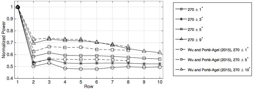
FIGURE 5. Comparison of the normalized mean power output data obtained from the LES of Wu and Porté-Agel (2015) and the present simulations, for several wind sectors.

Wu and Porté-Agel (2015) used an AD approach similar to that used in this work, with aerodynamic loads computed based on the local flow velocities. Simple control schemes were also added to account for the dynamics of the rotor. Simulations were performed for each degree from 260° to 280°. The mean powers of a wind sector consist of averages of rotor powers from simulations for which the wind direction is within the considered wind sector; a wind sector of 10±° thus implies simulations from 260° to 280°, including these two wind directions. The power output was averaged over a time of 40 min. Again, details about the averaging procedure in Wu and Porté-Agel (2015) are scarce: it is only mentioned that the power output of each row is obtained by averaging power of the eight lines at the row r. Only the power output for the first eight rows were shown in the paper.

In Figure 5, we notice small differences between our power production and that of Wu and Porté-Agel (2015). First of all, as already mentioned, we perform a simulation every two degrees, which is coarser than the wind direction discretization of other LES results (one simulation each 1°). For narrow wind sectors (up to ±5°), our results produce slightly lower levels of power than those reproduced from Wu and Porté-Agel (2015). A larger number of simulations could help in reducing these discrepancies. However, mainly for narrow wind sectors, the present results lead to a different behavior for the fourth row and the following ones. Our simulations predict a slightly lower production for these rotors, while a plateau in power production is reached from the third one for Wu and Porté-Agel. This cannot be attributed solely to a difference in the discretization. We propose several potential explanations:

• First of all, the grid used by Wu and Porté-Agel (2015) is coarser than the one used in the present simulations (more than twice as coarse); this impacts the rotor production but also the numerical and the subgrid scale dissipations. One can thus expect such a coarse grid to produce a different wake behavior, in terms of wake meandering, velocity recovery or level of turbulence. Narrow wind sectors exacerbate the sensitivity of the production prediction to the numerically-predicted wake characteristics as the downwind machines are most of the time fully or partially immersed in the wake. Larger wind sectors imply wind directions for which the rotors are not aligned anymore: the turbines are then more often out of the wake and impacted by the freestream flow. The impact of coarser grids may then be less significant, which might explain the better agreement between the LES results for wider wind sectors. A simulation on coarser mesh should be performed, to clearly identify the impact of the resolution on the power production.

• Secondly, the level of turbulence in our simulations is about 6.3% while that of simulations of Wu and Porté-Agel (2015) is about 7.7%. This can affect the production of the first machines: the second row of rotors may produce less (our simulations lead to a second row that produces slightly less than those of Wu and Porté-Agel (2015) simulations for 270 ± 3°), so the third one produces slightly more and the fourth one thus produces less. The plateau is then reached from the fourth row on. This could also explain the discrepancies observed in the comparison with measurements, as the observations are selected when the turbulence intensity is about 8%, which is slightly higher than that obtained in our simulations.

• Finally, there are also differences in the rotor representation. The rotor inertia is not represented in Wu and Porté-Agel (2015). Indeed, at each LES time step, the rotor speed is adapted instantaneously through an iterative procedure to produce the optimal torque based on the local flow velocities. The optimal behavior is thus achieved at every time step of the simulation. In our control architecture, as detailed in Supplementary Appendix 1, the rotor speed dynamics responds to the imbalance between the AD aerodynamic torque and the controlled generator torque. As the inertia is taken into account, the control takes several LES time steps to find the optimal rotor speed that balances the aerodynamic and the generator torques for the considered wind conditions. As a consequence, in the presence incoming flow velocity variations, the response of our controller and that of Wu and Porté-Agel (2015) will be different. This clearly affects the power output, and may explain the difference of powers observed in Figure 5.

4.2 Moments Histories and Correlations With Wake Meandering

We now investigate the history of the moments for several wind turbines and two representative and “extreme” wind directions: α = 270°, corresponding to the fully-aligned configuration, and α = 262°, where the rotors can be out of the upstream wakes during large periods. We consider four rotors, located in R₁, R₂, R₆ and R₁₀ in the middle line L₄ (see Figure 1 for the locations of those wind turbines). These rows are representative of the typical behaviors inside the wind farm, with rotors impacted by an unperturbed wind flow (R₁) or by a very well-structured wake (R₂) and with machines located deeper in the wind farm (R₆ and R₁₀). For α_w = 262°, the row R₁₀ may also correspond to situations where the machine is impacted by the wakes of the adjacent line.

We report on Figures 6, 7 the instantaneous signals of the root bending moments and the yaw and tilt moments. The histories of the flapwise and the edgewise root bending moments are shown for one blade, and are denoted M_f,1 and M_e,1, respectively. For the sake of clarity, we only show the instantaneous signals for 15 min. The time is made dimensionless by multiplying it by ${\bar{U}}_{hub}/D$ and is denoted t^*. The filtered signals, at the rotation frequency (f_Ω) for M_f,1 and M_e,1, and at three times f_Ω for M_y and M_t, are added on Figures 6, 7 in order to highlight the low frequency fluctuations of the moments.

FIGURE 6

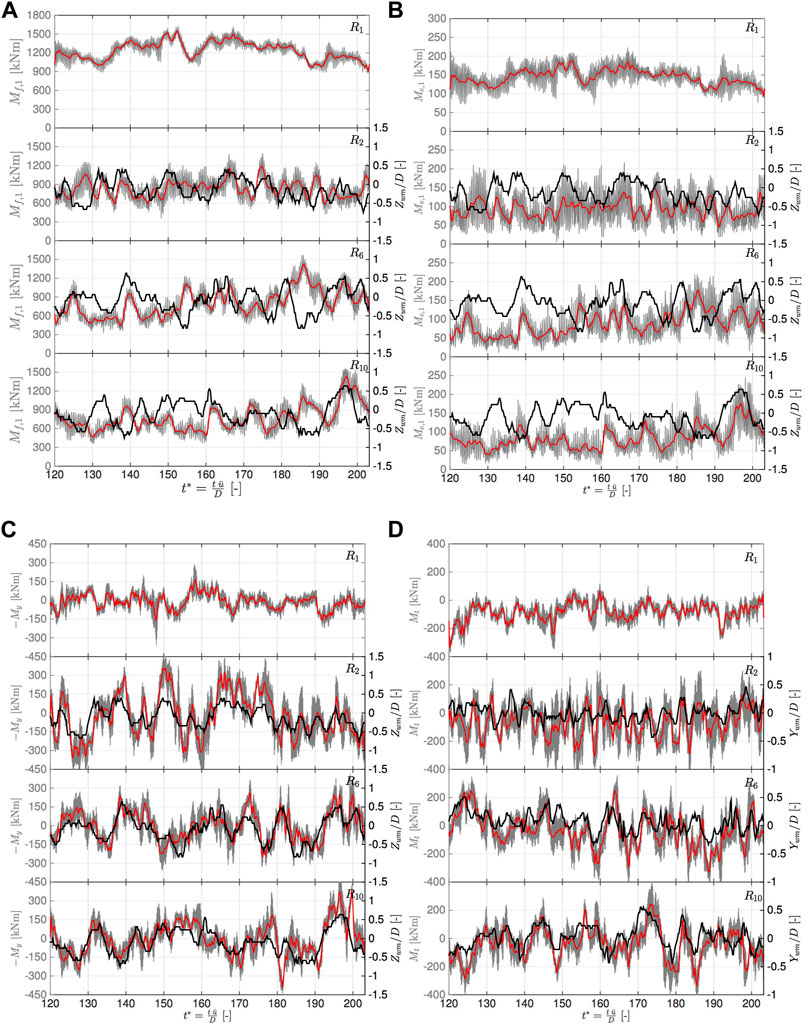
FIGURE 6. Histories of the flapwise (A) and edgewise (B) root bending moments and of the yaw (C) and tilt (D) moments for α_w = 270° and rows R₁, R₂, R₆ and R₁₀ (grey lines). The filtered signals of M_f,1 and M_e,1 at f_Ω, and of M_y and M_t at 3f_Ω are also added (red lines). The wake centerline position just upstream of the machine is also reported for rows R₂, R₆ and R₁₀ (black lines).

FIGURE 7

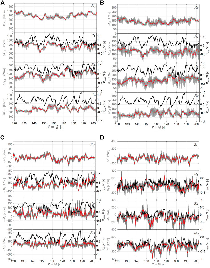
FIGURE 7. Histories of the flapwise (A) and edgewise (B) root bending moments and of the yaw (C) and tilt (D) moments for α_w = 262° and rows R₁, R₂, R₆ and R₁₀ (grey lines). The filtered signals of M_f,1 and M_e,1 at f_Ω, and of M_y and M_t at 3f_Ω are also added (red lines). The wake centerline position just upstream of the machine is also reported for rows R₂, R₆ and R₁₀ (black lines).

For rows R₂, R₆ and R₁₀, we also report on Figures 6, 7, the horizontal position of the wake center (denoted Z_wm) just upstream of the rotor, in order to discuss the moment behaviors with respect to the upstream wake movement. Z_wm is calculated as the relative horizontal position of the upstream wake with respect to the center of the rotor, and normalized by the Vestas diameter. For the tilt moment, it is more interesting to discuss its behavior as a function of the vertical upstream wake movement, denoted Y_wm. Y_wm is calculated as the relative vertical position of the upstream wake with respect to the hub height, and, again, it its normalized by the rotor diameter.

Additionally, we report on Figure 8 snapshots of the instantaneous streamwise velocities at several times, in order to support our discussion of some particular behaviors of the moments for the different machines. We also add the horizontal wake centerlines on those velocity slices.

FIGURE 8

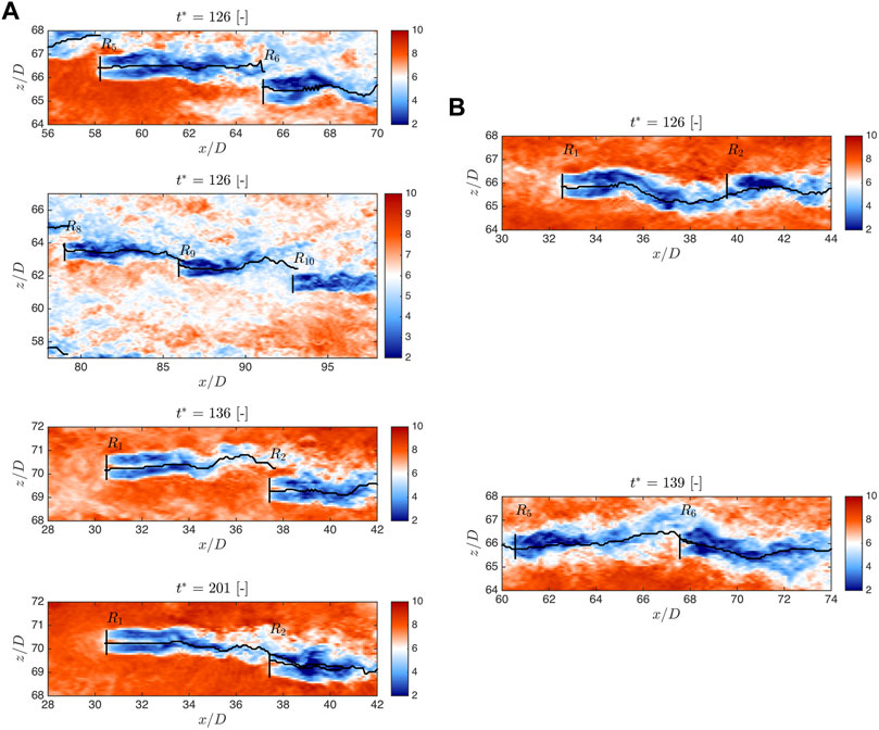
FIGURE 8. Several snapshots of the streamwise velocity in a horizontal plane located at hub height, centered around some rows, for wind directions α_w = 262° (A) and α_w = 270° (B). The units are in [m/s].

We structure our discussion in terms of 1) the depth of the turbines, and 2), the center of partial wake impingement (respectively, 270° or 262°).

Rows R₁ and R₂: For α_w = 270°, there is an increase in the amplitude of the high frequency oscillations of the root bending moments between R₁ and R₂ (see Figures 6A,B). Those moment fluctuations, denoted here as the 1P oscillations, are characterized by a frequency equal to that of the blade rotation and are due to the blade passage through areas of higher and lower velocities over one rotation. For row R₁, those oscillations occur when the rotor is partially immersed in a gust or in a lull and when the blade crosses the sheared wind. For row R₂, those moment fluctuations are mainly due to the presence of an upstream wake, which, at times, partially immerses the rotor. An example of the wind turbine in a half-wake situation is shown in Figure 8B for t^* = 126, which can be correlated with the high amplitudes of the high frequency moment fluctuations. For the considered wind conditions (${\bar{U}}_{hub}$ of 8 m/s and low TI), the wake downstream of the first wind turbine in a line is very “well-structured”, with a velocity deficit that is clearly more marked than the ambient wind fluctuations (as highlighted in Figure 3). The amplitude of the moment fluctuations for a rotor impacted by such a wake is thus higher than that observed when the machine is partially impacted by a gust. Moreover, Figure 6 shows that the meandering of the wake upstream of row R₂ is weak, with very small oscillations of the wake center: the rotor of R₂ is thus often in half wake situations, leading to many episodes of large-amplitude high-frequency moment fluctuations. This is also translated by a decrease of the time-averaged values of M_f,1 and M_e,1.

We also notice on Figures 6A,B, for row R₂, lower frequency fluctuations of M_f,1 and M_e,1 (highlighted in the filtered signals). This is due to the transition between full and half wake situations, characterized by a decrease and an increase in the mean values of M_f,1 and M_e,1.

For the yaw and tilt moments and α_w = 270° (see Figures 6A,B), there is also an increase in the amplitude of the fluctuations related to the blade rotation (the frequency of those oscillations is here equal to three times the rotation frequency (3P), as opposed to above (1P)). There is also a significant increase in the amplitude of the lower frequency fluctuations (see red curves of Figures 6A,B). For M_y, we see that those oscillations follow the horizontal wake movement, therefore at a frequency that is close to that of the wake meandering. As R₂ is fully aligned with R₁, M_y remains centered around zero, and oscillates between positive and negative values, depending on the wind turbine side impacted by the wake. The tilt moment is also correlated to the horizontal wake movement, but the correlation is more obvious when we consider the vertical wake movement (see Figure 6D). So, even if the vertical wake movement is small, its impact remains important, mainly in a configuration where the rotor is most of the time impacted by the wake.

The behavior of M_f,1, M_e,1, M_y and M_t is different for α_w = 262°. As the wind turbine of R₂ is misaligned with respect to that of R₁, it is often fully out of the upstream wake, making its behavior more similar to a machine of row R₁. For example, in Figure 7, between t^* = 135 and 145, we see that the moments have oscillations with means and amplitudes that are similar to those of row R₁: this can be linked to the wake centerline position, which is highly off-centered from the rotor hub at this particular time (see Figure 8A for t^* = 136). However, the wind direction α_w = 262° still leads to situations where the wind turbine of row R₂ is immersed in the upstream wake. For example, around t^* = 200, the center of the upstream wake is closer to that of the rotor, resulting in an increase in the amplitude of the high frequency oscillations for all the moments. It is also highlighted in the streamwise velocities at t^* = 201, reported in Figure 8A. As for α_w = 270°, there is an increase in the amplitude of the lower frequency oscillations, correlated to the horizontal motion of the upstream wake. For M_f,1 and M_e,1, those fluctuations occur at the same frequency as that of the wake meandering, as the wind turbine is off-centered from the upstream wake, and thus oscillates between periods where it is partially immersed in the wake and periods where it is fully out of the wake. The difference of the mean value around which the signal oscillates during these different periods can be large, as the rotor switches from a freestream situation, with high velocities, especially if it is impacted by a gust, to a waked configuration (for example between t^* = 145 and 155, in Figures 7A,B).

For M_y, the mean of the signal varies between zero (when the rotor is out of the wake) and negative values, as the wake only impacts one side of the rotor. For M_t, the correlation between the low frequency oscillations and the vertical wake movement is less obvious, as the wind turbine is either out of the wake, or partially immersed in the upstream wake.

Row R₆: For α_w = 262°, the behavior of row R₆ is comparable to that of row R₂, as the upstream wakes that impact these two rows have a similar behavior (see Figure 3A for the global view of the wind farm). However, the wake upstream of row R₆ is slightly less structured, and wider: so, even when the wake centerline is estimated far from the rotor center, the rotor can be still impacted by some flow structures of the wake, as highlighted for t^* = 126 and row R₆ in Figure 8A. For α_w = 270°, compared to α_w = 262°, the behavior of the upstream wake differs more between R₂ and R₆. The amplitude of the wake meandering increases, leading to a wind turbine that is sometimes out of the upstream wake (for example around t^* = 139, see Figure 8B). However, as the wake is more destructured and also wider, the rotor blade crosses wake structures most of the time, even when the center of wake is computed as being far from the rotor one. This decreases the amplitude of the moment fluctuations related to the blade passage and, mainly for the yaw moment, those of lower frequencies, correlated to the wake meandering. As the wake also recovers faster deeper in the wind farm, the velocities in the wake upstream of row R₆ are higher, further attenuating the high frequency moment fluctuations occurring when the rotor is in half wake situation.

Row R₁₀: For α_w = 270°, the behavior of the wind turbine of row R₁₀ is globally similar to that of R₆. For α_w = 262°, as already mentioned, in addition to the upstream wakes of its own line, R₁₀ is also impacted by the wakes of the adjacent line L5 (see Figure 3 the global view of the wind farm). The rotor is then immersed in a more “uniform flow”, with changes in velocity speed that are less marked, as it is well noticeable in Figure 8A for t^* = 126 and R₁₀. This decreases the amplitude of the moment oscillations at the blade passage frequency, but also at lower frequencies, correlated to the large scale wake motion.

It is relevant to compare the LES results to those obtained with the actual measurements available in Hansen et al. (2014). Their work studied the flapwise root bending moment for the wind turbine located in R₂ and L₄ as a function of the different atmospheric stabilities and incoming wind speeds and directions. The wind speed was estimated based on the measurement at the nacelle of that wind turbine, while the wind direction was derived from pairs of undisturbed wind turbines assuming no yaw misalignment. The atmospheric stability was estimated based on the Monin-Obukhov theory and wind speed, air and see temperatures, all measured at met mast 7 (see Figure 1).

For wind directions that led it to freestream conditions and for 8 m/s, the wind turbine of R₂ and L₄ exhibits a measured time-averaged flapwise bending moment of slightly less than 1,400 kNm. These particular operating conditions can be related to those of R₁ in our simulations, which corresponds to a freestream turbine. We obtain a time-averaged value that is equal to 1,250 kNm for this particular turbine, which underpredicts the mean M_f by about 10% compared to the measurements. The discrepancies between the LES results and the measurements may be explained in several manners. First, although a large part of the study of Hansen et al. (2014) was dedicated to the dependence of the fatigue loads to the atmospheric stability, it seems that the time-averaged value was computed from all the valid measurements, and not only from those representative of the neutral atmospheric stability. The atmospheric stability impacts the wind shear and the turbulence intensity, which may lead to differences in the resulting time-averaged M_f. Additional discrepancies may come from to the establishment of the inflow flow characteristics. As mentioned, the wind speed is measured at the nacelle of the wind turbine. For wind speeds below 11 m/s, the authors mention that the measurement at the nacelle matches well with the ambient flow when the wind turbine is in freestream condition. However, it is not specified if a correction accounting for the rotor induction, potential pressure gradients around the nacelle or wake effects (because the anemometer is located behind the blades) exists. This contributes to increase the uncertainties, which are not quantified in Hansen et al. (2014).

We also compare the time-averaged M_f for R₂ and α_w = 270° to that obtained with the actual measurements of Hansen et al. (2014) for the same machine. For a mean wind speed of about 5.5 or 6 m/s, corresponding to the upstream velocity of R₂ in our LES results, Hansen et al. (2014) obtained a value between 700 and 800 kNm for wind directions that set the wind turbine in fully aligned conditions. The LES results produce a time-averaged value of about 900 kNm, which corresponds to an error between 13 and 22%. This difference can be explained in several manners. First, the measurements were given for fully aligned conditions, which led to the lowest separation between wind turbines (i.e., 7D), but it was not explicitly mentioned in Hansen et al. (2014) whether these conditions accounted for α_w = 270° only. Other wind directions satisfy that criterion (e.g., α_w = 90°), and result in a different relative wind turbine position within the wind farm, and thus a different M_f behavior. Again, the uncertainties related to the estimation of the inflow characteristics may reinforce the discrepancies. The atmospheric stability also plays an important role, as it impacts the upstream wake behavior. We recall that no distinction was made between the stability types for the computation of the time-averaged value given in Hansen et al. (2014).

4.3 Load Cycle Distribution

We now investigate the number of cycles, n_i, per moment amplitude M_i, computed using the Rainflow counting (RFC) method (ASTM A. E, 2003). We sill consider the wind directions α_w = 262° and 270° and the rows R₁, R₂, R₆ and R₁₀. In order to have consistent n_i in the large moment amplitudes, which are marginally captured by the simulations, we accumulate the cycles over six lines, from L₂ to L₇. We deliberately omit L₁ and L₈ in the computation, as they potentially have a different behavior, due to their position at the extremities of the wind farm. The resulting cycle distributions are reported on Figure 9, for the four moments. For the root bending moments, the cycles are moreover accumulated over the three blades: those moments are now denoted M_f and M_e. Again, the discussion follows a row-wise order.

FIGURE 9

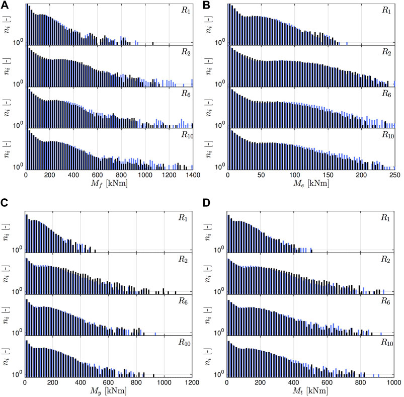
FIGURE 9. Number of cycles for the flapwise (A) and edgewise (B) root bending moments and for the yaw (C) and tilt (D) moments in the rows R₁, R₂, R₆, and R₁₀, for α_w = 262° (blue bars) and α_w = 270° (black bars). For each row, the number of cycles is accumulated over six lines, from L₂ to L₇.

Rotors of row R₁: Globally, as expected, the cycle distribution for row R₁ is similar for the two considered wind directions. The small discrepancies observed in n_i are due to the change of the rotor location according to the wind direction. We notice a peak in n_i for moments of middle amplitudes. As already mentioned, this results from the moment fluctuations when the blades crosse long-lasting areas of higher and lower velocities over their rotation.The cycles of large amplitude are due to more global changes in the incoming wind speed, i.e. larger gust or lulls.

Rotors of row R₂: For the four investigated moments and the two wind directions, the distribution of n_i varies between R₁ and R₂. The number of load cycles of middle and large amplitudes increases, and the peak related to the blade rotation is shifted towards higher moment amplitudes, and spread over a wider range of moments. As already highlighted in the discussion about the instantaneous signals, it is due to the presence of an upstream wake, characterized by a velocity deficit that is clearly more marked than the ambient wind fluctuations.

Compared to α_w = 262°, the root bending moments obtained for α_w = 270° have a higher number of cycles around the middle amplitudes for M_f and M_e, with a peak that is slightly shifted towards higher amplitudes. This is due to the high frequency moment oscillations that have, for most of the simulation time, higher amplitudes than for α_w = 262°, as highlighted in Section 4.2. For α_w = 270° and M_e, the amplitude of the lower frequency oscillations, which are the same order of magnitude as those of higher frequency, contributes to increase the peak. For M_f in particular, α_w = 262° seems to lead to higher maximal amplitudes, although the number of those cycles remains small. It is due to the transitions between periods where the rotor is immersed in the wake, and periods where the rotor is out of the wake, as highlighted in Section 4.2. For α_w = 270°, M_y and M_t also present a non-zero number of cycle in the very large amplitudes, which may contribute to increase the differences in the resulting fatigue loads between the two different directions.

Rotors of row R₆: For α_w = 262°, the n_i distribution for R₆ is comparable to that observed for row R₂, as the upstream wakes impacting these two rows globally have a similar behavior (see Figure 3A). For α_w = 270°, compared to row R₂, R₆ sees an upstream wake with a lower velocity deficit and that is wider, which reduces the amplitude of the 1P and 3P moment fluctuations when it is fully and partially immersed in wake and thus shifts the distribution towards lower moment amplitudes. The tail of the M_f cycle distribution also spreads over larger amplitudes: as the amplitude of the wake meandering upstream increases, the wind turbine located in R₆ is sometimes out of the wake, increasing the amplitude of the low frequency oscillations when the it transits between waked and freestream situations. In contrast, the cycle distribution of M_e remains compact and does not extend to larger cycle amplitudes. Indeed, for M_e, compared to M_f, the amplitude of the low frequency fluctuations is closer to that of the 1P oscillations. In fact, it is even of the same order of magnitude as that of the 1P oscillations of row R₂ (see Figure 6B). Consequently, the increase in the amplitude of the lower frequency oscillations between R₂ and R₆ does not contribute to spread the cycle distribution over large amplitudes. For M_y, if the wind turbine is more often completely out-of-wake, this will decrease the amplitude of the lower frequency oscillations due to an imbalance in the rotor loads (highlighted Figure 6C), moving the cycle distribution towards smaller amplitudes. For M_t, the tail of the distribution still extends to cycles with amplitudes similar to those of R₂. However, Figure 6D highlights that, between R₂ and R₆, there is a net decrease in the frequency of the filtered moment fluctuations. Those fluctuations were correlated to the vertical wake movement for R₂. As R₆ is more often out of the wake, this is translated by a decrease in the number of cycles of about 400 or 500 kNm, and a decrease in the resulting fatigue damage (this will be discussed in Section 4.4).

Rotor of row R₁₀: For α_w = 270°, R₁₀ presents a similar cycle distribution as for row R₆. For α_w = 262°, as R₁₀ is impacted by the wakes of its own line, but also those of the adjacent line L₅, the rotor is then immersed in a more “uniform flow”, decreasing number of cycles n_i in the large amplitudes.

4.4 Fatigue Equivalent Loads

In order to investigate the effects of the wind direction and the wind turbine location on the resulting fatigue damages, a quantitative fatigue indicator, the equivalent moment M_eq, is here computed. M_eq is estimated based on the cycle distribution computing using the RFC method, combined with a Palmgren-Miner rule Miner (1945). Assuming that the moment is proportional to the stress, M_eq is computed as

$M_{eq}={\left(\sum _{i=1}^{L_c}\frac{n_i{M}_i^m}{N_{eq}}\right)}^{\frac{1}{m}}(10)$

where i and L_c represent the load case number and the total number of load cases, respectively; n_i is the number of cycles for the particular moment amplitude M_i, determined using the RFC method; m is a parameter dependent on the material; N_eq is an arbitrary number of cycles. As we only investigate M_eq as ratios, N_eq does not need to be defined in this work. In the present study, M_i corresponds to a particular M_f, M_e, M_y or M_t amplitude. The exponent m is here defined as 10 for M_f and M_e, which is a widely used value for blades made of fiberglass (Mandell and Samborsky, 1997), such as those of the Vestas 2 MW. The yawing and tilting moments impact, among other components, the main shaft, which is usually made in forged steel (AWEA, BlueGreen, GLWN, and NIST, 2011): m is chosen to be equal to 4, which is within the range between 3 and 5 typically used for the metallic wind turbine components (Guideline and Lloyd, 2010). In each line, the fatigue estimate is normalized by M_eq of the first row. We still accumulate the cycles from line L₂ to line L₇, and also over the three blades for M_f and M_e.

We organize the discussion around these four equivalent moments shown in Figure 10.

Flapwise moment M_eq,f: Globally, for the two wind directions, there is a marked increase in M_eq,f between the first row and the downstream rows. This is an expected behavior after the discussions of Sections 4.2 and 4.3. Compared to α_w = 270°, α_w = 262° leads to a higher increase in the equivalent M_f for rows R₂ to R₆, despite its smaller n_i in the small and middle amplitudes (see Figure 9A). Indeed, for this wind direction, the number of cycles in the very large moment amplitudes is non-zero. Even if their numbers are small, those cycles are particularly significant in the fatigue estimates, notably due to the presence of the m exponent in the computation of M_eq. From row R₇ for α_w = 262°, the rotors are additionally impacted by the wakes of the adjacent lines, slightly reducing the number of large amplitude cycles, and shifting the peak related to the blade rotation towards lower amplitudes (see discussion of Section 4.3). As a consequence, the resulting fatigue damage decreases, and becomes smaller than that obtained for α_w = 270°. For α_w = 270°, although the cycle distribution is slightly shifted towards lower amplitudes for rows downstream of R₂, it is also spread over larger amplitudes (as highlighted in Figure 9A). As a consequence, the ratios $M_{eq,f,R_i}/M_{eq,f,R_1}$ still increase after row R₂.

Edgewise moment M_eq,e: The increase in M_eq,e is similar in both wind directions, excepted for rows R₇ to R₁₀, where the fatigue estimates is lower for α_w = 262°. For both wind directions, R₂ presents the highest increase in M_eq. Indeed, for rows located downstream, the cycle distribution is shifted towards lower amplitudes, without an increase in the number of cycles of large amplitude, as highlighted in Figure 9B for R₆ and R₁₀ and in the discussion of Section 4.3.

Yaw and tilt moments, M_eq,y and M_eq,t: For α_w = 270°, the increase in the fatigue damage due to M_y and M_t is more important than that obtained for α_w = 262°. It was highlighted in the discussion of the instantaneous signals in Section 4.2. The fatigue damages also slightly decrease for rows located deeper in the wind farms. Again, this was highlighted in Figure 9 and in the discussion of Section 4.3. For α_w = 262°, the equivalent moments slightly increase between row R₃ and R₆, and, again, decrease for the last rows.

It is relevant to compare the increase in fatigue equivalent loads to results available in the literature. To that end, the ratio of flapwise equivalent loads between R₁ and R₂ as a function of the incoming wind direction is reported in Figure 11. We here consider all the simulated wind directions; in order to make clearer the comparison with other results, the wind direction is expressed as the offset with respect to α_w = 270°. We also report on Figure 11 the results of Lee et al. (2018). Lee et al. (2018) numerically investigated the damage equivalent loads in a pair of floating wind turbines. The first wind turbine and its resulting wake were simulated using LES coupled to an AL model. The behavior of the second wind turbine was modeled by extracting time series of a planar data at 7D downstream from the turbine to use as an input to FAST. They made vary the lateral position of the downstream wind turbine, in order to simulate fully and partially immersed situations. They consider a turbine of 3MW, and thus with a radius larger than the Vestas 2MW, but, as mentioned, the spacing between the two wind turbines is 7D, which is equal to our configuration for α_w = 270°. Moreover, the wind speed is about 9 m/s, meaning that the rotor operates in the second region of the power curve, with a thrust coefficient close to that of our LES results. The TI is set to less than 4%, which is lower to the TI used in the Horns Rev simulations. This may lead to discrepancies between the two sets of results, as the TI affects the wake meandering. The comparison between the results should be also cautiously done, as Lee et al. (2018) consider floating wind turbines, capturing the interactions between the platform, the wake and the turbine. However, we expect a similar behavior in terms of the evolution of the fatigue damage.

FIGURE 10

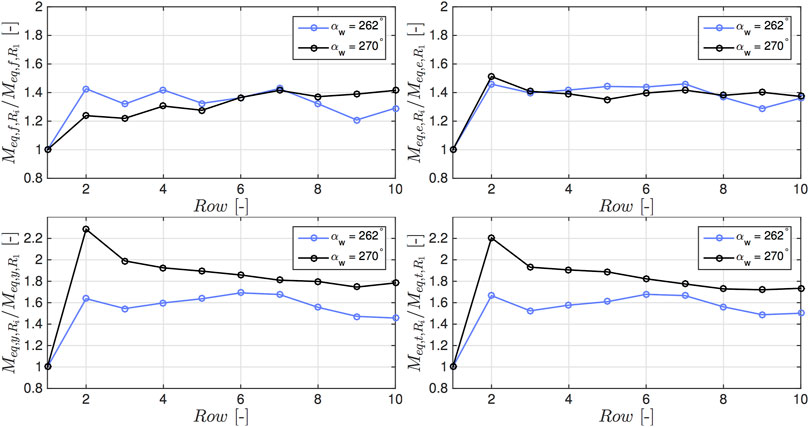
FIGURE 10. M_eq for the 10 rows, normalized by M_eq of the first row of the line for the wind directions 262° and 270°.

FIGURE 11

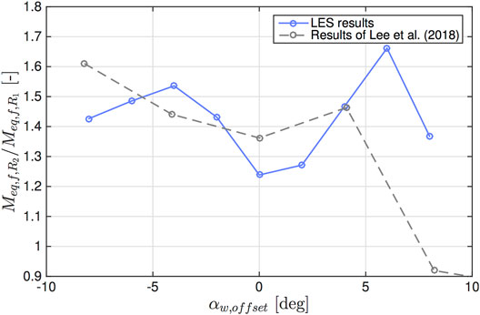
FIGURE 11. Flapwise equivalent moment of R₂, normalized by that of R₁, as a function of the incoming wind direction. The wind direction is expressed as the offset with respect to 270°. The results of Lee et al. (2018) are also reported; the ratios are computed based on the absolute values available in Lee et al. (2018).

Globally, we see the same tendency for both sets of results, with a lower increase of M_eq for fully aligned conditions than for small offsets. This tendency is also observed in other research works (Schmidt et al., 2011). Indeed, when the wind turbine is fully aligned with the upstream machine, there are periods where the rotor remains fully immersed in the upstream wake, decreasing the flow variations that the blade crosses over one rotation. The amplitude of the load cycles associated to those 1P oscillations is thus smaller, which decreases the resulting damage equivalent loads. For small offset (e.g., + or -5°), as the wind turbine is most of time partially immersed in the upstream wake, the increase in fatigue loads is more significant. When the offset increases, the rotor is more often out of the wake (this was well highlighted in the discussion of Sections 4.2 and 4.3), which decreases the damage equivalent loads. However, for an offset of about 8°, we see in Figure 11 that there are more discrepancies between the two sets of results. Lee et al. (2018) explained their low increase in M_eq for that offset by a wake deficit region that was non-symmetric due to its interaction with the vertical shear and the presence of the Coriolis effect. We do not account for the Coriolis forces in our LES, which may explain that the wake remains more symmetric, and that we do not observe a net decrease for the positive offset of about 8°. However, for the other offsets, the order of magnitude of the increase of M_eq is globally similar in the two sets of results.

5 Conclusion

In this work, we proposed a methodology aiming at simulating the whole wind farm behavior, from the wake phenomena to the wind turbine fatigue loads, in a both accurate and efficient way and for a large range of operating conditions. We used Large Eddy Simulation (LES), coupled to an Actuator Disk (AD) approach. The use of the AD method allows for coarse resolutions and thus reduces the computational costs of the simulations. In order to recover pertinent fatigue loads with that model, we replicated the blade trajectories through the disk and interpolated the AD aerodynamic forces onto these “virtual blades” at each time step. This allowed us to easily compute the resulting blade root bending and yaw and tilt moments. The wake centerline was also tracked in the whole wind farm, in order to highlight the correlations between the wake phenomena and the wind turbine fatigue damage.

We used the described methodology for simulating the Horns Rev wind farm for wind directions varying between 262° and 278°, with a simulation every 2°. 270° corresponds to a westerly wind, leading to the smallest spacing between wind turbines and a perfect alignment of the rotors in a line.

We first compared our time-averaged power production to the Horns Rev measurements of Barthelmie et al. (2009) and to other LES results (Wu and Porté-Agel, 2015), for different wind sectors. Discrepancies between the simulation results and the measurements for small wind sectors could be attributed to the uncertainties in the measured wind direction and possible yaw misalignment for the actual wind farm. Small discrepancies were also observed between the LES results and those of Wu and Porté-Agel (2015). These could be due to a difference of resolution, wind turbine controller, and additional small variations in the turbulence intensity of the freestream flow. Widening the wind sector brought to a very good agreement between our LES results, those of Wu and Porté-Agel (2015) and the measurements.

We then investigated the fatigue loads for several machines inside the wind farm and two particular wind directions, α_w = 270° and 262°. In this study, we considered the blade root bending moments and the yaw and tilt moments. We clearly showed the link between the upstream wake movement and the resulting high and low frequency oscillations of the investigated moments. The high frequency fluctuations were attributed to the load variation when the blade moved in and out of the wake when the wind turbine was in an half wake situation, while the lower frequency oscillations were due to the wake sweeping across the rotor plane. The time-averaged flapwise moments were also compared to actual measurements for a turbine in a freestream configuration and in waked situation. The differences varied between 13 and 22%, which was attributed to uncertainties related to the estimation of inflow conditions (atmospheric stability, wind speed and direction,…).

The load cycle distributions, computed using the Rainflow counting method, were also studied for the same machines and wind directions, and reflected the main behaviors observed in the moment history. The second row in a line saw its number of cycles increase in the middle and large amplitudes, due to the presence of upstream wakes. This contributed to increasing the rotor fatigue damage, as highlighted in the resulting equivalent moment. For α_w = 262°, until the seventh row in a line, the equivalent moments are more less equal to those of the second row. From the seventh row, the rotors were also impacted by the wakes of the adjacent line, making the flow field more uniform, reducing the equivalent moments. For α_w = 270°, the equivalent moments slightly decreased after the second row, because the upstream wakes were less structured and characterized with a lower velocity deficit. This reduced the amplitude of the high and low frequency oscillations of the moments.

We also compared the ratios of flapwise equivalent moments between the first and the second rows for all the simulated wind directions, to those of other numerical studies. Those studies did not simulate the Horns Rev wind farm in particular, but considered a pair of wind turbines, with different lateral positions for the downstream machine. In this analysis, we saw that our results globally reproduced the same tendency and the same order of magnitude for the ratios.

Although the proposed methodology could be further improved by coupling the flow solver to an aeroelastic code, or by accounting for different atmospheric stabilities and Coriolis effects, the numerical tool clearly demonstrated its capacity to accurately capture the wind farm flow and the wind turbine fatigue loads. Compared to lower fidelity approaches, such as a wake model coupled to a Blade Element Momentum (BEM), it captures all the fine physics of the wake phenomena, and its impact on the turbine loads. It also remains computationally affordable at the scale of a large wind farm scale, unlike LES coupled to an Actuator Line method, which requires finer spatio-temporal resolutions. As our tool also includes the tracking of the wake centerline position, it identifies the correlations between fatigue loads and wake phenomena, and highlights the flow features that should be captured by operational wake models in a perspective of model predictive control of the wind farm. In this study in particular, we highlight the signature of the wake meandering during full or partial impingement scenarios, wake merging contribution for the deeper rows, and in particular, its signature in the load cycle distribution.

Data Availability Statement

The raw data supporting the conclusions of this article will be made available by the authors, without undue reservation.

Author Contributions

MM performed the simulations, the post-processing of the results and discussed the results. PC supervised the modelling work, and contributed to the results analysis and discussion.

Funding

This project has received funding from the European Research Council (ERC) under the European Union’s Horizon 2020 research and innovation program (grant agreement no. 725627). Simulations were performed using computational resources provided by the Consortium des Équipements de Calcul intensif (CÉCI), funded by the Fonds de la Recherche Scientifique de Belgique (F.R.S.-FNRS) under Grant No. 2.5020.11, and computational resources made available on the Tier-1 supercomputer of the Fédération Wallonie-Bruxelles, infrastructure funded by the Walloon Region under the Grant Agreement No. 1117545.

Conflict of Interest

The authors declare that the research was conducted in the absence of any commercial or financial relationships that could be construed as a potential conflict of interest.

Publisher’s Note

All claims expressed in this article are solely those of the authors and do not necessarily represent those of their affiliated organizations, or those of the publisher, the editors and the reviewers. Any product that may be evaluated in this article, or claim that may be made by its manufacturer, is not guaranteed or endorsed by the publisher.

Supplementary Material

The Supplementary Material for this article can be found online at: https://www.frontiersin.org/articles/10.3389/fenrg.2022.881532/full#supplementary-material

References

ASTM A. E (2003). 1049–standard Practices for Cycle Counting in Fatigue Analysis. West Conshohocken (PA).

Google Scholar

Aubrun, S., Muller, Y. A., and Masson, C. (2015). Predicting Wake Meandering in Real-Time through Instantaneous Measurements of Wind Turbine Load Fluctuations. J. Phys. Conf. Ser. 625, 012005. doi:10.1088/1742-6596/625/1/012005

CrossRef Full Text | Google Scholar

AWEA, BlueGreen, GLWN, and NIST (2011). Wind Energy Industry Manufacturing Supplier Handbook. Tech. Rep.USA: AWEA.

Google Scholar

Bangga, G., and Lutz, T. (2021). Aerodynamic Modeling of Wind Turbine Loads Exposed to Turbulent Inflow and Validation with Experimental Data. Energy 223, 120076. doi:10.1016/j.energy.2021.120076

CrossRef Full Text | Google Scholar

Barthelmie, R. J., Frandsen, S. T., Rathmann, O., Hansen, K. S., Politis, E., Prospathopoulos, J., et al. (2011). “Flow and Wakes in Large Wind Farms: Final Report for UpWind WP8,” in Tech. rep., Danmarks Tekniske Universitet, Risø Nationallaboratoriet for Bæredygtig Energi.

Google Scholar

Barthelmie, R. J., Hansen, K., Frandsen, S. T., Rathmann, O., Schepers, J. G., Schlez, W., et al. (2009). Modelling and Measuring Flow and Wind Turbine Wakes in Large Wind Farms Offshore. Wind Energy 12, 431–444. doi:10.1002/we.348

CrossRef Full Text | Google Scholar

Barthelmie, R. J., Pryor, S. C., Frandsen, S. T., Hansen, K. S., Schepers, J. G., Rados, K., et al. (2010). Quantifying the Impact of Wind Turbine Wakes on Power Output at Offshore Wind Farms. J. Atmos. Oceanic Tech. 27, 1302–1317. doi:10.1175/2010JTECHA1398.1

CrossRef Full Text | Google Scholar

Barthelmie, R. J., Rathmann, O., Frandsen, S. T., Hansen, K. S., Politis, E., Prospathopoulos, J., et al. (2007). Modelling and Measurements of Wakes in Large Wind Farms. J. Phys. Conf. Ser. 75, 012049. doi:10.1088/1742-6596/75/1/012049

CrossRef Full Text | Google Scholar

Bossanyi, E. (2018). Combining Induction Control and Wake Steering for Wind Farm Energy and Fatigue Loads Optimisation. J. Phys. Conf. Ser. 1037, 032011. doi:10.1088/1742-6596/1037/3/032011

CrossRef Full Text | Google Scholar

Bottasso, C. L., Cacciola, S., and Schreiber, J. (2018). Local Wind Speed Estimation, with Application to Wake Impingement Detection. Renew. Energ. 116, 155–168. doi:10.1016/j.renene.2017.09.044

CrossRef Full Text | Google Scholar

Capello, E., Wada, T., Punta, E., and Fujisaki, Y. (2020). Trade‐off between Power Extraction Maximisation and Fatigue Reduction in Wind Farms via Second‐order Sliding Mode Control and Min-max Optimisation. IET Control. Theor. Appl 14, 2535–2547. doi:10.1049/iet-cta.2019.1088

CrossRef Full Text | Google Scholar

Caprace, D.-G., Winckelmans, G., and Chatelain, P. (2020). An Immersed Lifting and Dragging Line Model for the Vortex Particle-Mesh Method. Theor. Comput. Fluid Dyn. 34, 21–48. doi:10.1007/s00162-019-00510-1

CrossRef Full Text | Google Scholar

Chatelain, P., Duponcheel, M., Zeoli, S., Buffin, S., Caprace, D.-G., Winckelmans, G., et al. (2017). Investigation of the Effect of Inflow Turbulence on Vertical axis Wind Turbine Wakes. J. Phys. Conf. Ser. 854, 012011. doi:10.1088/1742-6596/854/1/012011

CrossRef Full Text | Google Scholar

Churchfield, M. J., Lee, S., Moriarty, P. J., Hao, Y., Lackner, M. A., Barthelmie, R., et al. (2015). A Comparison of the Dynamic Wake Meandering Model, Large-Eddy Simulation, and Field Data at the Egmond Aan Zee Offshore Wind Plant. Tech. Rep. NREL/CP-5000-63321, NREL/CP-5000-63321. doi:10.2514/6.2015-0724

CrossRef Full Text | Google Scholar

Cosack, N. (2010). Fatigue Load Monitoring with Standard Wind Turbine Signals. Ph.D. thesis, Stuttgart University.

Google Scholar

Coudou, N., Moens, M., Marichal, Y., Van Beeck, J., Bricteux, L., and Chatelain, P. (2018). Development of Wake Meandering Detection Algorithms and Their Application to Large Eddy Simulations of an Isolated Wind Turbine and a Wind Farm. J. Phys. Conf. Ser. 1037, 072024. doi:10.1088/1742-6596/1037/7/072024

CrossRef Full Text | Google Scholar

Damiani, R., Dana, S., Annoni, J., Fleming, P., Roadman, J., van Dam, J., et al. (2018). Assessment of Wind Turbine Component Loads under Yaw-Offset Conditions. Wind Energ. Sci. 3, 173–189. doi:10.5194/wes-3-173-2018

CrossRef Full Text | Google Scholar

Dao, C., Kazemtabrizi, B., and Crabtree, C. (2019). Wind Turbine Reliability Data Review and Impacts on Levelised Cost of Energy. Wind Energy 22, 1848–1871. doi:10.1002/we.2404

CrossRef Full Text | Google Scholar

Duponcheel, M., Bricteux, L., Manconi, M., Winckelmans, G., and Bartosiewicz, Y. (2014). Assessment of RANS and Improved Near-wall Modeling for Forced Convection at Low Prandtl Numbers Based on LES up to Reτ=2000. Int. J. Heat Mass Transfer 75, 470–482. doi:10.1016/j.ijheatmasstransfer.2014.03.080

CrossRef Full Text | Google Scholar

Duponcheel, M., Orlandi, P., and Winckelmans, G. (2008). Time-reversibility of the Euler Equations as a Benchmark for Energy Conserving Schemes. J. Comput. Phys. 227, 8736–8752. doi:10.1016/j.jcp.2008.06.020

CrossRef Full Text | Google Scholar

España, G., Aubrun, S., Loyer, S., and Devinant, P. (2011). Spatial Study of the Wake Meandering Using Modelled Wind Turbines in a Wind Tunnel. Wind Energy 14, 923–937. doi:10.1002/we.515

CrossRef Full Text | Google Scholar

Galinos, C., Dimitrov, N., Larsen, T. J., Natarajan, A., and Hansen, K. S. (2016). Mapping Wind Farm Loads and Power Production - A Case Study on Horns Rev 1. J. Phys. Conf. Ser. 753, 032010. doi:10.1088/1742-6596/753/3/032010

CrossRef Full Text | Google Scholar

Gao, X., Wang, T., Li, B., Sun, H., Yang, H., Han, Z., et al. (2019). Investigation of Wind Turbine Performance Coupling Wake and Topography Effects Based on Lidar Measurements and Scada Data. Appl. Energ. 255, 113816. doi:10.1016/j.apenergy.2019.113816

CrossRef Full Text | Google Scholar

Guideline, G., and Lloyd, G. (2010). Guideline for the Certification of Wind Turbines. Tech. Rep. Hamburg: Germanischer Lloyd Wind Energie Gmb H.

Google Scholar

Hansen, K. S., Barthelmie, R. J., Jensen, L. E., and Sommer, A. (2012). The Impact of Turbulence Intensity and Atmospheric Stability on Power Deficits Due to Wind Turbine Wakes at Horns Rev Wind Farm. Wind Energy 15, 183–196. doi:10.1002/we.512

CrossRef Full Text | Google Scholar

Hansen, K. S., Larsen, G. C., and Ott, S. (2014). Dependence of Offshore Wind Turbine Fatigue Loads on Atmospheric Stratification. J. Phys. Conf. Ser. 524, 012165. doi:10.1088/1742-6596/524/1/012165

CrossRef Full Text | Google Scholar

Hansen, M. H., Hansen, A. D., Larsen, T. J., Øye, S., Sørensen, P., and Fuglsang, P. (2005). Control Design for a Pitch-Regulated, Variable Speed Wind Turbine. Tech. rep., DTU.

Google Scholar

Harrison, M., Bossanyi, E., Ruisi, R., and Skeen, N. (2020). An Initial Study into the Potential of Wind Farm Control to Reduce Fatigue Loads and Extend Asset Life. J. Phys. Conf. Ser. 1618, 022007. doi:10.1088/1742-6596/1618/2/022007

CrossRef Full Text | Google Scholar

Hegazy, A., Blondel, F., Cathelain, M., and Aubrun, S. (2022). Lidar and Scada Data Processing for Interacting Wind Turbine Wakes with Comparison to Analytical Wake Models. Renew. Energ. 181, 457–471. doi:10.1016/j.renene.2021.09.019

CrossRef Full Text | Google Scholar

Herges, T. (2018). Results from the SWiFT Wake Steering Experiment. Tech. Rep. Albuquerque, NM (United States): Sandia National Lab.SNL-NM.

Google Scholar

Jin, M., and Yang, X. (2021). A New Fixed‐point Algorithm to Solve the Blade Element Momentum Equations with High Robustness. Energy Sci Eng 9, 1734–1746. doi:10.1002/ese3.945

CrossRef Full Text | Google Scholar

Jonkman, J., and Buhl, J. M. L. (2005). FAST Users Guide. Tech. Rep. TP-500-38230. NREL.

Google Scholar

Kanev, S. K., Savenije, F. J., and Engels, W. P. (2018). Active Wake Control: An Approach to Optimize the Lifetime Operation of Wind Farms. Wind Energy 21, 488–501. doi:10.1002/we.2173

CrossRef Full Text | Google Scholar

Kim, Y., Jost, E., Bangga, G., Weihing, P., and Lutz, T. (2016). Effects of Ambient Turbulence on the Near Wake of a Wind Turbine. J. Phys. Conf. Ser. 753, 032047. doi:10.1088/1742-6596/753/3/032047

CrossRef Full Text | Google Scholar

Larsen, G. C., Aagaard Madsen, H., and Bingöl, F. (2007). Dynamic Wake Meandering Modeling. Tech. Rep. Risø-R-1607 (EN). Risø National Laboratory.

Google Scholar

Larsen, T. J., Madsen, H. A., Larsen, G. C., and Hansen, K. S. (2013). Validation of the Dynamic Wake Meander Model for Loads and Power Production in the Egmond Aan Zee Wind Farm. Wind Energy 16, 605–624. doi:10.1002/we.1563

CrossRef Full Text | Google Scholar

Lee, M. J., Oh, B. D., and Kim, Y. B. (2001). Canonical Fractional-step Methods and Consistent Boundary Conditions for the Incompressible Navier-Stokes Equations. J. Comput. Phys. 168, 73–100. doi:10.1006/jcph.2000.6682

CrossRef Full Text | Google Scholar

Lee, S., Churchfield, M., Driscoll, F., Sirnivas, S., Jonkman, J., Moriarty, P., et al. (2018). Load Estimation of Offshore Wind Turbines. Energies 11, 1895. doi:10.3390/en11071895

CrossRef Full Text | Google Scholar

Lejeune, M., Moens, M., Coquelet, M., Coudou, N., and Chatelain, P. (2020). Data Assimilation for the Prediction of Wake Trajectories within Wind Farms. J. Phys. Conf. Ser. 1618, 062055. doi:10.1088/1742-6596/1618/6/062055

CrossRef Full Text | Google Scholar

Liu, Z., Li, Q., Ishihara, T., and Peng, J. (2020). Numerical Simulations of Fatigue Loads on Wind Turbines Operating in Wakes. Wind Energy 23, 1301–1316. doi:10.1002/we.2487

CrossRef Full Text | Google Scholar

Madsen, H. A., Larsen, T. J., Pirrung, G. R., Li, A., and Zahle, F. (2020). Implementation of the Blade Element Momentum Model on a Polar Grid and its Aeroelastic Load Impact. Wind Energ. Sci. 5, 1–27. doi:10.5194/wes-5-1-2020

CrossRef Full Text | Google Scholar

Mandell, J. F., and Samborsky, D. D. (1997). DOE/MSU Composite Material Fatigue Database: Test Methods, Materials, and Analysis (Sandia National Laboratories Albuquerque).

Google Scholar

Mann, J. (1998). Wind Field Simulation. Probabilistic Eng. Mech. 13, 269–282. doi:10.1016/S0266-8920(97)00036-2

CrossRef Full Text | Google Scholar

Martínez-Tossas, L., and Leonardi, S. (2013). “Wind Turbine Modeling for Computational Fluid Dynamics,” in Tech. Rep. SR-5000-55054. NREL.

Google Scholar

Meng, H., Li, L., and Zhang, J. (2020). A Preliminary Numerical Study of the Wake Effects on the Fatigue Load for Wind Farm Based on Elastic Actuator Line Model. Renew. Energ. 162, 788–801. doi:10.1016/j.renene.2020.07.140

CrossRef Full Text | Google Scholar

Miner, M. A. (1945). Cumulative Damage in Fatigue. J. Appl. Mech. 12, A159–A164. doi:10.1115/1.4009458

CrossRef Full Text | Google Scholar

Moens, M., Coquelet, M., Trigaux, F., and Chatelain, P. (Forthcoming 2022a). Handling Individual Pitch Control within an Actuator Disk Framework: Verification against the Actuator Line Method and Application to Wake Interaction Problems. J. Phys. Conf. Ser.

Google Scholar

Moens, M., Duponcheel, M., and Chatelain, P. (Forthcoming 2022b). Assessment of an Actuator Disk-Based Approach for the Prediction of Fatigue Loads in a Perspective of Wind Farm Scale Application. Wind Energy.

Google Scholar

Moens, M., Duponcheel, M., Winckelmans, G., and Chatelain, P. (2018). An Actuator Disk Method with Tip-Loss Correction Based on Local Effective Upstream Velocities. Wind Energy 21, 766–782. doi:10.1002/we.2192

CrossRef Full Text | Google Scholar

Moens, M. (2018). Large Eddy Simulation of Wind Farm Flows - Improved Actuator Disk Model and Investigations of Wake Phenomena. Ph.D. thesis, École polytechnique de Louvain-Universitćatholique de Louvain.

Google Scholar

Monaghan, J. J. (1985). Extrapolating B Splines for Interpolation. J. Comput. Phys. 60, 253–262. doi:10.1016/0021-9991(85)90006-3

CrossRef Full Text | Google Scholar

Movsessian, A., Schedat, M., and Faber, T. (20202020). Modelling tower Fatigue Loads of a Wind Turbine Using Data Mining Techniques on Scada Data. Wind Energ. Sci. Discuss., 1–20.

Google Scholar

Muller, Y.-A., Aubrun, S., and Masson, C. (2015). Determination of Real-Time Predictors of the Wind Turbine Wake Meandering. Exp. Fluids 56, 53. doi:10.1007/s00348-015-1923-9

CrossRef Full Text | Google Scholar

Munters, W., Meneveau, C., and Meyers, J. (2016). Turbulent Inflow Precursor Method with Time-Varying Direction for Large-Eddy Simulations and Applications to Wind Farms. Boundary-layer Meteorol. 159, 305–328. doi:10.1007/s10546-016-0127-z

CrossRef Full Text | Google Scholar

Naughton, B. T. (2017). “Test Plan for the Wake Steering Experiment at the Scaled Wind Farm Technology (SWiFT) Facility,” in Tech. Rep. SAND2017-1730. SANDIA. doi:10.2172/1367493

CrossRef Full Text | Google Scholar

Park, J., Basu, S., and Manuel, L. (2014). Large-Eddy Simulation of Stable Boundary Layer Turbulence and Estimation of Associated Wind Turbine Loads. Wind Energy 17 (3), 359–384.

CrossRef Full Text | Google Scholar

Potentier, T., Braud, C., Guilmineau, E., Finez, A., and Le Bourdat, C. (2021). Analysis of the DANAERO Wind Turbine Field Database to Assess the Importance of Different State‐of‐the‐art Blade Element Momentum (BEM) Correction Models. Energ. Sci Eng 9, 1477–1500. doi:10.1002/ese3.908

CrossRef Full Text | Google Scholar

Riva, R., Liew, J., Friis-Møller, M., Dimitrov, N., Barlas, E., Réthoré, P.-E., et al. (2020). Wind Farm Layout Optimization with Load Constraints Using Surrogate Modelling. J. Phys. Conf. Ser. 1618, 042035. doi:10.1088/1742-6596/1618/4/042035

CrossRef Full Text | Google Scholar

Schmidt, B., Lloyd, G., Schmidt, B., King, J., Hassan, G. G., King, J., et al. (2011). Wake Loads and Fatigue Load Certification in Offshore Wind Farms. Offshore EWEA Proc.

Google Scholar

Sheng, S. (2013). “Report on Wind Turbine Subsystem Reliability-A Survey of Various Databases (Presentation),” in Tech. Rep. Golden, CO (United States): National Renewable Energy Lab.NREL.

Google Scholar

Simley, E., Fleming, P., Girard, N., Alloin, L., Godefroy, E., and Duc, T. (2021). Results from a Wake-Steering experiment at a Commercial Wind Plant: Investigating the Wind Speed Dependence of Wake-Steering Performance. Wind Energ. Sci. 6, 1427–1453. doi:10.5194/wes-6-1427-2021

CrossRef Full Text | Google Scholar

Smagorinsky, J. (1963). General Circulation Experiments with the Primitive Equations. Mon. Wea. Rev. 91, 99–164. doi:10.1175/1520-0493(1963)091<0099:gcewtp>2.3.co;2

CrossRef Full Text | Google Scholar

Stanley, A. P. J., King, J., and Ning, A. (2020). Wind Farm Layout Optimization with Loads Considerations. J. Phys. Conf. Ser. 1452, 012072. doi:10.1088/1742-6596/1452/1/012072

CrossRef Full Text | Google Scholar

Thiry, O. (2017). Direct and Large-Eddy Simulation of Turbulent wall-bounded Flows - Further Development of a Parallel Solver, Improvement of Multi Scale Sub Grid Models and Investigation of Vortex Pairs in Ground Effects. Ph.D. thesis, École polytechnique de Louvain-Universitćatholique de Louvain.

Google Scholar

Trujillo, J.-J., Bingöl, F., Larsen, G. C., Mann, J., and Kühn, M. (2011). Light Detection and Ranging Measurements of Wake Dynamics. Part Ii: Two-Dimensional Scanning. Wind Energy 14, 61–75. doi:10.1002/we.402

CrossRef Full Text | Google Scholar

Van der Hooft, E., Schaak, P., Van Engelen, T., et al. (2003). Wind Turbine Control algorithmsDOWEC Project-DOWEC-F1w1-EH-03-094/0, Task-3 Report.

Google Scholar

van Dijk, M. T., van Wingerden, J.-W., Ashuri, T., and Li, Y. (2017). Wind Farm Multi-Objective Wake Redirection for Optimizing Power Production and Loads. Energy 121, 561–569. doi:10.1016/j.energy.2017.01.051

CrossRef Full Text | Google Scholar

Vasilyev, O. V. (2000). High Order Finite Difference Schemes on Non-uniform Meshes with Good Conservation Properties. J. Comput. Phys. 157, 746–761. doi:10.1006/jcph.1999.6398

CrossRef Full Text | Google Scholar

Vera-Tudela, L., and Kühn, M. (2017). Analysing Wind Turbine Fatigue Load Prediction: The Impact of Wind Farm Flow Conditions. Renew. Energ. 107, 352–360. doi:10.1016/j.renene.2017.01.065

CrossRef Full Text | Google Scholar

Vollmer, L., Steinfeld, G., Heinemann, D., and Kühn, M. (2016). Estimating the wake deflection downstream of a wind turbine in different atmospheric stabilities: an les study. Wind Energ. Sci. 1, 129–141. doi:10.5194/wes-1-129-2016

CrossRef Full Text | Google Scholar

Wu, Y.-T., and Porté-Agel, F. (2015). Modeling Turbine Wakes and Power Losses within a Wind Farm Using LES: An Application to the Horns Rev Offshore Wind Farm. Renew. Energ. 75, 945–955.doi:10.1016/j.renene.2014.06.019

CrossRef Full Text | Google Scholar