 Kuo-Hua Huang
 Kuei-Hsiang Chao
- Department of Electrical Engineering, National Chin-Yi University of Technology, Taichung, Taiwan
The main purpose of this study is to engage in research on a grid-connected photovoltaic (PV) power generation system smart inverter. The research content includes a smart maximum power point tracking (MPPT) controller and an inverter with power regulation. First, use the PSIM software package to establish the simulation environment of the grid-connected photovoltaic power generation system and use the Sanyo HIP-186BA19 photovoltaic module to form a 744 W system for simulation. In order to enable the photovoltaic module array (PVMA) to output the maximum power under different solar insolation and ambient temperature, the architecture is based on the extension theory-based smart MPPT method to improve the dynamic response and steady-state performance of photovoltaic power generation systems compared to perturb and observed (P&O) MPPT. When the sunshine is 1,000 W/m2, the photovoltaic power generation system adopts the extension theory-based maximum power tracking method. The time required to track the maximum power point is only 0.32 s, and the steady-state ripple is only 4.127 W. However, using the traditional P&O method requires 0.741 s to track the maximum power point, and the steady-state ripple reaches 18.131 W. Thus, the dynamic response speed of the maximum power tracking method proposed is 50% faster than that of the P&O method. The steady-state performance is also better compared to the P&O method. At the same time, a simple proportional-integral (PI) controller is used to regulate the DC-link voltage, output voltage, and current of the inverter to make the voltage of the grid-connected point stable at an effective value of 220 V. Then, the voltage-power control technology is added to the photovoltaic grid-connected inverter, and a simple proportional-integral controller is used to regulate the output of the smart inverter reactive power to improve the power quality of grid voltage. Finally, simulation and experimental results are used to verify the effectiveness of the regulation performance of the developed smart inverter.
1 Introduction
In order to reduce the burden of the public power supply system during peak power consumption, energy storage systems are generally used, or other alternative energy sources, such as batteries or photovoltaic systems, are generally used to solve this problem. A power conditioner must be used for power conversion to convert the energy in the battery energy storage system or the energy of the photovoltaic system into electrical energy for general electrical appliances. If the electricity generated by the photovoltaic power generation system is converted and then sent back to the grid power, the power supplier will no longer be the grid power but the load of the power conditioner (Urakabe et al., 2010). The advantage of the grid-connected photovoltaic system is that when the power generation of the system is not enough for the user, the user can supplement the power shortage from the grid power; conversely, when the power converted by the system is surplus, it can be fed back to the power company. The power company can not only reduce the demand for peak power consumption from the grid power but also save the power company’s additional generator sets from supplying only a few hours of peak electricity consumption per day, as well as reducing fuel consumption and carbon dioxide emissions (Usher and Martel, 1994). Its applicable location can be installed in the place where the public power system can be normally reached. The advantages are a simple system, easy maintenance, and photovoltaic inverters’ conversion efficiency as high as 98% (Pearsall, 2017). Nevertheless, the disadvantage of this type of grid-connected system is that, in order to prevent equipment damage or jeopardizing personnel safety due to islanding operation, the photovoltaic inverter automatically shuts down the grid-connected power supply. Hence, no electricity is available, so it does not have a disaster prevention function. Therefore, the main function of the photovoltaic inverter is to convert the photovoltaic energy after the maximum power tracking into a sinusoidal AC power source and supply it to the power grid. The control goal of the system is to control the amplitude, frequency, and phase of the output voltage to be consistent with the power grid, and the system’s power factor (PF) is 1.
Because the photovoltaic module is a non-ideal direct current type, it is greatly affected by the amount of sunlight and the module’s temperature. Therefore, in order to achieve the maximum power output of the photovoltaic power generation system, the maximum power tracking technology must be used. Given the above situation, various studies have proposed various smart maximum power tracking methods for photovoltaic module arrays when shading and failure conditions occur. Among them, the more common ones are ant colony optimization (ACO) (Saoji and Rao, 2021), artificial bee colony algorithms (ABC) (Xue et al., 2021), adaptive velocity particle swarm optimization (AVPSO) (Pragallapati et al., 2017), and modified particle swarm optimization (PSO) (Sen et al., 2018). Still, the calculation of these smart algorithms is quite complicated, so it takes much time to track the maximum power point, which will affect the tracking speed.
In addition, because the output of the photovoltaic power generation system is an unstable direct current (DC) source, it is necessary to convert the DC source into a stable alternating current (AC) source through an inverter to supply power in parallel with the grid power. However, when more photovoltaic power generation systems are parallel connected to the public power grids, the characteristics of the photovoltaic power generation system that change with the amount of sunlight and the temperature of the module will cause serious changes in the grid power voltage, resulting in poor power quality. Therefore, the smart inverter must implement active power and reactive power to regulate control to maintain a stable voltage supply. Accordingly, this study focuses on the maximum power tracking method of the photovoltaic module array, the configuration design of the DC/AC conversion inverter (Bletterie et al., 2010), and the active power and reactive power control of the smart inverter.
The extension theory-based maximum power tracking method has been proposed in this study to improve the dynamic tracking response and steady-state performance of the P&O method. In addition, in order to improve the power supply quality of the PV grid-connected system, a smart inverter has been developed to commence voltage-power control at the output end, thereby providing stable voltage for the grid-connected system.
2 Constructing an Extension Theory-Based Maximum Power Tracking
This study first uses the PSIM simulation software package (PSIM Website, 2022) to establish an equivalent circuit model of the photovoltaic module for Sanyo HIP-186BA19 (SANYO HIP-186BA19 Data Sheet, 2014). Its output characteristic curve is the same as in actual operation. A 744W photovoltaic module array is established with a rated output voltage of 217.6 V (four modules in serial) and a rated output current of 3.71 A (one module in parallel), and the extension theory (Yang and Zhang, 2011) was applied to track the maximum power point under different sunshine intensity and module temperature. Extension theory has now been widely used in practice and research in professional fields such as decision-making, search, and fault diagnosis. Therefore, this study uses the smart maximum power tracking method based on the perturb and observe (P&O) (Verma et al., 2017) and extension theory to conduct the maximum power tracking of the photovoltaic module array so as to accurately track the maximum power point of the photovoltaic module array. This study establishes extension element models for each maximum power tracking control category. Based on the extension method, the slope error, and slope error variation value in the power-voltage (P-V) characteristic curve of the photovoltaic module array to capture the classical and neighborhood domains of the signal characteristic value, the membership function was applied to calculate the membership grade for each category and accordingly determine the control category, thereby returning the pulse width modulation (PWM) trigger signal to the DC/DC boost converter and then controlling the turn-on and turn-off time of the power semiconductor switch to track the maximum power point (MPP).
2.1 Extension Theory
Extension theory can be divided into extension mathematics and matter-element theory. Extension mathematics takes extension set and extension correlation function as the main indicators. Moreover, matter-element theory divides an object into characteristics and the range value of characteristic expansion through the matter-element model in the extension theory to represent its object information. By transforming the relationship of the objects, it is possible to know the proportion of each characteristic that affects the objects and clearly observe the importance of characteristics to the objects.
The matter-element model: the matter element is the basic element used to describe “objects,” determined by the name (N) of the objects, its characteristics (C), and the corresponding value (V). These three basic elements are composed to describe objects, and the matter element is represented by R, which is expressed in the mathematical model as follows:
where R is the basic element to describe objects, called matter element, and the three basic matter elements are the name N, characteristics C, and characteristic value V of objects.
2.1.1 Definition of Distance
Let x be any point on the real domain (−∞, +∞) and X0 = <a, b> any interval on the real field, called the distance between point x and interval X0. The following equation present point x and interval X0 relationship:
2.1.2 Definition of Position Value
Let x be any point on the real domain (−∞, +∞); X0 = <a, b>, X = <c, d>, X0 ⊂ X are the two intervals on the real domain; and for the position value of point x related to X0, X can be expressed as follows:
2.1.3 Definition of Correlation Function
The function composed of the distance divided by the position value is called the elementary correlation function, and its expression is shown as follows:
K(x) is the element x about the interval X0, X correlation function. When the value of the correlation function is larger, the degree of correlation between the element and this interval is better.
2.2 Maximum Power Tracking Method Based on Extension Theory
This study combines the extension theory as the theoretical basis and proposes a smart maximum power tracking method (Chao et al., 2011; Chao et al., 2012). Analyze the P-V characteristic curve of the photovoltaic module array, take the slope error and the slope error change as the characteristics of the extension maximum power tracking method, and set up 12 categories and establish their matter-element models to calculate the correlation between them. Adjust the duty cycle (D) of the MPPT converter according to its category to achieve maximum power tracking (Chao and Li, 2010).
The characteristics of the extension theory maximum power tracking method are the slope error е, the slope error variation Δе, and the duty cycle variation ΔD. Figure 1 is a schematic diagram of the change of the slope error е and the slope error variation Δе of the P-V characteristic curve. Based on the P-V characteristic curve of the photovoltaic module array, two characteristics [slope error e (k) and the slope error change Δe(k)], defined in Eqs 5–7, have been divided into 12 categories. For example, for category #1, if slope error e is a positive and small value and the slope error change Δe is a native value, the operation point is on the left of the maximum power point (MPP). When it is close to the MPP, the increased voltage of the photovoltaic module arrays (PVMAs) can be controlled to shift the operation point to the right to track MPP. This will reduce the duty cycle of the boost converter, leading to a decrease in the output current of the module array. Accordingly, the output voltage of the PV module array will increase. As the operation point in category #1 is quite close to MPP, the duty cycle only needs to be slightly decreased to slightly increase the voltage of the PVMA. The operation point can then shift to the MPP in small steps, not likely causing great oscillation to and from the MPP or causing power generation loss. Therefore, if the operation point is in category #1, ΔD = −0.001. In other categories, the ΔD positive and negative values and sizes are determined by the same method. Take the operation point farther away from the left side of MPP as an example. In order to quickly track MPP, the voltage of the PVMA must be substantively increased. Therefore, the duty cycle D is substantively reduced, making the ΔD negative value enlarged, such as category #3 in Figure 1. At this time, ΔD = −0.05. On the contrary, for the operation point farther away from the right side of MPP, in order to quickly track MPP from the left side, the voltage of the photovoltaic module array must be substantively reduced. Therefore, the duty cycle D of the boost converter needs to be amplified, leading to a substantial increase in the output current of the PV module array. The output voltage of the PV module array can be quickly lowered, prompting the operation point to quickly shift toward the direction of MPP on the left side. By considering #12 in the category in Figure 1, for example, e is a negative value and Δe is a positive value. However, the operation point is on the right of the MPP and farthest away from MPP. Therefore, ΔD = +0.05 (positive maximum) is set. The slope error, slope error variation, and duty cycle variation of each category are shown in Table 1. According to the P-V characteristic curve of the photovoltaic module array obtained during solar irradiation 200 ∼1,000
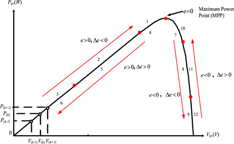
FIGURE 1. Schematic diagram of the slope error е and slope error change Δе of the P-V characteristic curve.
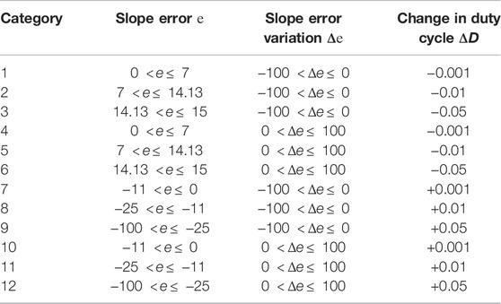
TABLE 1. Slope error, slope error variation, and duty cycle variation of 12 categories.
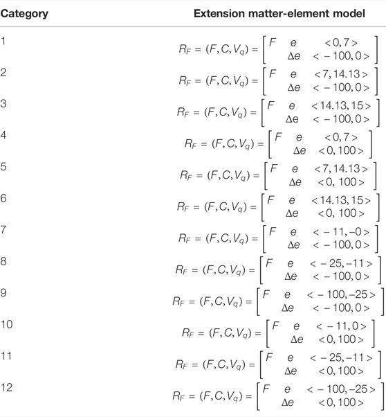
TABLE 2. Extension matter-element models of 12 categories.
2.3 Boost Converter
Figure 2 is the architecture diagram of the maximum power tracking system based on the extension theory. A boost converter is designed between the photovoltaic power generation system and the load (Chao and Lee, 2011). The duty cycle D of the converter is changed to track the maximum power point of the photovoltaic power generation system.
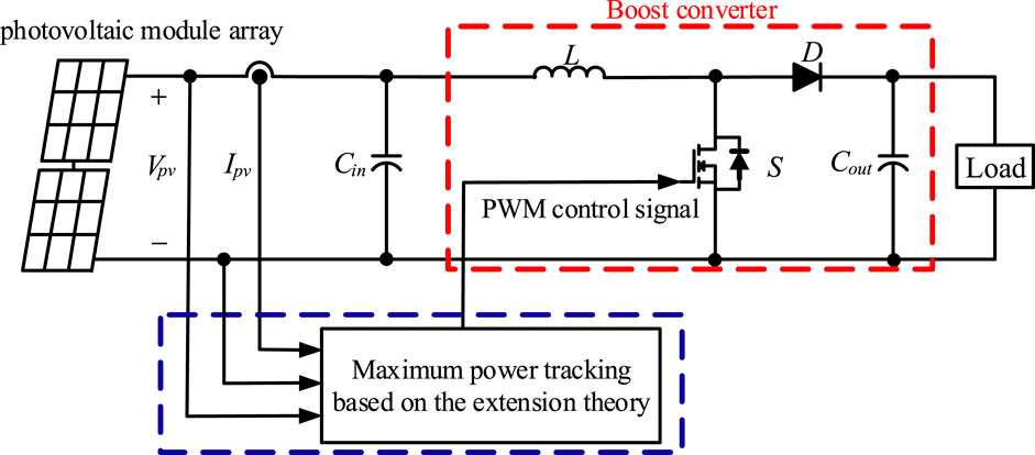
FIGURE 2. Maximum power tracking system architecture based on the extension theory.
The boost converter in this study is designed in continuous conduction mode (CCM); that is, the operating conditions are
From the function
The operating frequency of the maximum power tracking controller used in this paper is 20 kHz. Because the operating power of the subsequent test system is about 750 W, the rated power P of the converter is set to 900 W, and the maximum output operating voltage Vo is 400 V, which is determined by R = Vo2/P and can calculate the resistance value of load R to be 178 Ω. Then, calculate the required L value of 329 μH according to Eq. 9, and then multiply this L value by a margin of 1.25 times to ensure that the inductor current operates in continuous conduction mode. Hence, the inductor value selected in this study is 0.5 mH.
The change in charge of the capacitor during the on-time of the switch is (Hart, 2016)
where
Select the switch and the component part of the diode because the withstand voltage of both must be greater than the output voltage of 400 V when it is turned off. According to Hart (2016), calculate the switch component. The current rating needs to be greater than Imax (2.93A). Based on the convenience of laboratory acquisition, IRFP460 is selected as the switching element, and its specification is 500 V/20 A. The selected diode is FMPG5FS, and its specification is 1500 V/10 A.
3 Smart Inverter Control Architecture
In the research of smart photovoltaic inverters, this study focuses on the smart inverter with an input DC-link voltage of 400 V and output capacity of 744 VA. It connects its output to a single-phase 60 Hz/220
In the future, more photovoltaic power generation systems will be parallel connected to the grid power. If they supply too much or too little energy to the grid power, the voltage of the grid power will rise or fall. At this time, the smart inverter will detect the level of the grid power voltage. The output power is controlled by generating or absorbing the reactive power of the power grid connected to effectively restrain the grid power voltage from stabilizing at a normal value and achieve the balance adjustment of the supply and demand of the power grid.
3.1 Control Architecture of a Single-Phase Photovoltaic Full-Bridge Inverter
This study proposes a single-phase full-bridge inverter circuit structure, as shown in Figure 3, for converting the DC power of the photovoltaic module to the power grid, which uses dual-loop control. The outer loop is a DC-link voltage loop, using the error between the reference voltage (here is set to 400 V) and the practical output voltage of the DC link to generate the current command of the inner loop. The inner loop is the inverter output voltage and current control loop, and the error is used to generate the PWM control signal to control the AC output voltage. PWM adopts the sine wave pulse width modulation switching method to generate the trigger signal of the switch, and Lf -Cf constitutes a low pass filter to attenuate the high-frequency switching of the inverter. The output end makes the output voltage a sine wave of the grid power frequency.
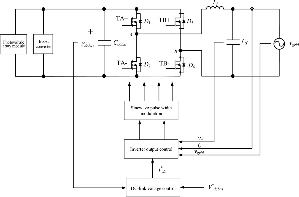
FIGURE 3. Circuit architecture of a single-phase photovoltaic full-bridge inverter.
3.1.1 DC-Link Voltage Control
In the photovoltaic power generation system, the photovoltaic module array is greatly affected by the sunlight and the module temperature. The output voltage and output current show a nonlinear relationship, so the characteristic curve is not the same. In order to make the photovoltaic module array output the maximum power, the duty cycle of the boost converter is controlled by the maximum power tracking method based on the extension theory so that the photovoltaic array module output power can reach the maximum power point. Still, it will make the output voltage of the converter an unstable DC voltage, which causes the DC voltage at the input end of the inverter to be unstable. Therefore, in order to stabilize the input DC voltage of the inverter, the control of the DC-link voltage (He et al., 2011) at the input end of the inverter becomes very important. First, after calculating the error between the DC-link voltage at the input of the actual inverter and the set voltage (set to 400 V in this study), the DC current command from the proportional-integral controller is used to generate a unit sine wave after zero detection with the utility power. When the DC-link voltage
The current command
where
3.1.2 AC Output Voltage and Current Control
The control architecture of this system adopts sinusoidal pulse width modulation (SPWM) technology and external voltage control and current control (Ciobotaru et al., 2005). The entire control system architecture is shown in the block diagram of Figure 4. In order to make the output voltage consistent with the power grid, the effective value is 220 V, so after calculating the error between the power grid voltage Vgrid and the inverter output voltage command
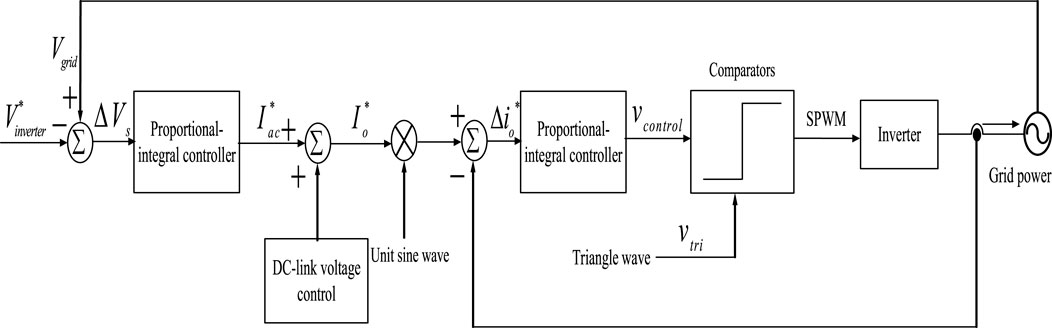
FIGURE 4. Single-phase photovoltaic inverter output control architecture.
It can be observed from Figure 4 that vcontrol can be obtained by Eqs 12–15. The PI controller in the serial shown in Eq.12 is adopted in this study. For the parameter values, proportional and integral constants are set, respectively, as KPv = 0.1 and KIv = 5 through try and error. An intelligent controller will be adopted in follow-up studies to enhance the robustness and adaptability of the controller:
where
3.2 Power Control of Single-Phase AC System
The inverter of the single-phase main system has only a single vector and cannot directly generate a dual-axis DC control system through Park’s transformation matrix (Krause et al., 2002). Therefore, if one wants to analyze the active power and reactive power of a single-phase system, one needs to use the imaginary quadrature-axis system (Azab, 2017). The single-phase inverter output voltage
Then, use the imaginary vector to generate the quadrature-axis (β-axis) component with a phase difference of 90o from the direct axis as
Therefore, the output voltage of the single-phase inverter can be expressed as
In the same way, the current components of the direct axis (α-axis) and the quadrature axis (β-axis) of the stationary reference frame of the single-phase inverter output current
Therefore, the output current of the single-phase inverter can be expressed as
Figure 5 is a schematic diagram of the single-phase inverter system vector projection on a stationary reference frame, so the system’s active power and reactive power can be obtained from Eq. 22 and Eq. 23, respectively. The active output power of the single-phase inverter can be expressed as
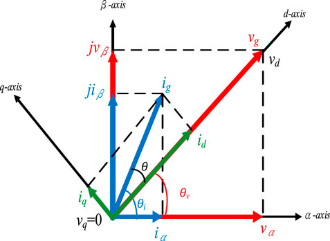
FIGURE 5. The relationship between decoupling control of single-phase inverter system on the reference coordinate axis.
In the same way, the instantaneous reactive power of the single-phase inverter system can be obtained as
From Eq. 22 and Eq. 23, the output active power and reactive power of the inverter can be calculated. When the direct-axis current component
From (Chen and Chien, 2014), we can use Park’s transformation to convert the stationary frame reference coordinate axis into a synchronous reference coordinate and fix the voltage vector
Eq. 23 can be simplified to
It can be seen from Eq. 25 that the active power and reactive power have been decoupled. The direct axis current
Figure 6 is a diagram of the structure controlling the output voltage and current phase angle difference of the smart inverter. After an error occurs in the command value of the reactive power, the direct-axis current command
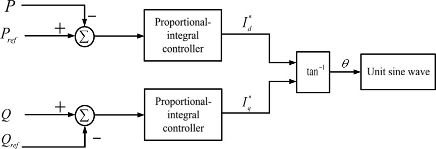
FIGURE 6. The architecture for controlling the phase angle difference of the output voltage and current of the smart inverter.
3.3 The Output Voltage-Power Control of the Smart Inverter
When the smart inverter is parallel-connected to the grid system, it must comply with the grid-connected regulations. Because several renewable energy sources are connected to the grid, the grid power voltage will fluctuate greatly. Therefore, it is necessary to pay attention to the requirements for voltage fluctuations in the grid-connected regulations. When the smart inverter starts to perform voltage-power control due to the fluctuation of the grid voltage, if the grid voltage or frequency still cannot operate stably and exceeds the normal range, the smart photovoltaic inverter must trip by itself to avoid damage.
After calculating the error between the actual grid power terminal voltage and the reference voltage (220 V), the reactive power command
Figure 7 is the voltage-power control flowchart. First, detect the voltage at the grid-connected point of the inverter, and perform reactive power control according to the grid power voltage per unit (p.u.). When equal to 1, the PF is maintained at 1. At this time, no reactive power is absorbed or provided, and only the active power is provided. When the per unit value of the grid power voltage is greater than 1 p.u. and less than 1.03 p.u., the PF will be controlled to decrease to 0.9 gradually (lagging). When the per unit value of the grid power voltage is greater than 0.97 p.u. and less than 1 p.u., the PF will be controlled to decrease to 0.9 gradually (leading). The above control adjusts the reactive power to return the grid power voltage normal range. However, if the power factor has been adjusted to 0.9 leading or lagging, the grid power voltage cannot effectively restrain its rise or fall, and when the system voltage is greater than 1.03 p.u. or less than 0.97 p.u., the photovoltaic power generation system will be disconnected from the grid system.
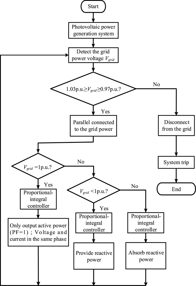
FIGURE 7. Voltage-power control flowchart.
4 Simulation Results
In this study, the photovoltaic module SANYO HIP-186BA19 is connected with four serial and one parallel to establish a 744 W photovoltaic module array. The electrical specifications are shown in Table 3. The parameter values of the boost converter and inverter are listed in Table 4. According to the different conditions of the amount of sunlight, the data acquisition of the P-V characteristic curve of the photovoltaic module array is carried out, and the matter-element model is established.
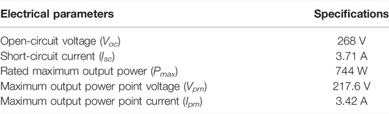
TABLE 3. Electrical specifications of SANYO HIP-186BA19 photovoltaic module array.
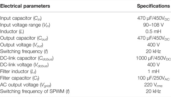
TABLE 4. The circuit parameters of the boost converter and inverter.
Because the single-phase smart photovoltaic inverter can provide and absorb the reactive power to the power grid system, it can stabilize the grid voltage. Therefore, in order to verify the control system and control method, a single-phase smart photovoltaic inverter system architecture was constructed with PSIM software. The voltage of the grid system is divided into three operating voltage ranges—1) Vgrid = 1 p.u., 2) 1.03 p.u. > Vgrid ≥ 1 p.u., and 3) 1 p.u. > Vgrid > 0.97 p.u.—and the smart inverter provides and absorbs reactive power to suppress or increase the grid system voltage effectively.
4.1 Maximum Power Tracking Simulation Results
Figure 8 shows the simulation waveforms of maximum power tracking using the traditional P&O and extension theory-based methods, respectively. It can be observed from Figure 8 that the convergence time of the P&O method is 0.741 s. However, the extension theory-based MPPT convergence time is 0.32 s. In particular, the perturbation factor in the P&O method is changed in the duty cycle of the boost converter, which is hereby set as △D = 0.02. As for the power ripple, when the P&O method is adopted, the value is 18.131 W. When the extension theory-based method is used, the value is only 4.127 W. The simulation results show that when the control system adopts the extension theory for MPPT, the output power of the photovoltaic module array can be quickly and stably controlled at the MPP
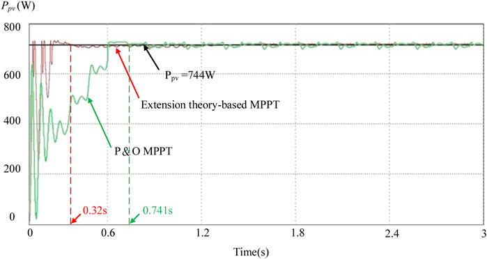
FIGURE 8. Simulation waveforms of the MPPT using the P&O and extension theory-based method when sunshine is 1,000 W/m2.

TABLE 5. A comparison of performance extension theory-based and P&O MPPT.
4.2 Simulation Results of Smart Inverter Control
4.2.1 The Per Unit Value of the Grid Voltage Is Equal to 1 p.u.
The smart photovoltaic inverter’s power factor will be maintained at 1 when it is detected that the grid voltage per unit value is equal to 1 p.u. Figure 9 shows the output power waveform of the smart inverter when the grid voltage per unit value is equal to 1 p.u. It can be observed from Figure 9 that the PV system does not provide or absorb any reactive power at this time but only provides active power to the grid. Figure 10 shows the output voltage and current of the smart inverter when the effective value of the grid voltage is 220 V. From Figure 10, the output voltage and current are in the same phase.
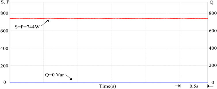
FIGURE 9. The output power of the smart inverter when the grid voltage per unit value is equal to 1 p.u.
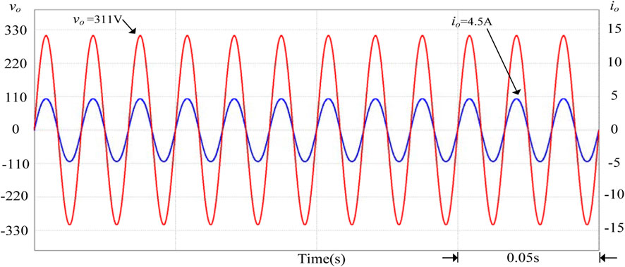
FIGURE 10. The output voltage and current waveforms of the smart inverter when the grid voltage per unit value is equal to 1 p.u.
4.2.2 The Per Unit Value of Grid Voltage Is Between 1 and 1.03 p.u.
If too much renewable energy is parallel connected to the grid when the amount of sunshine gradually rises, the power injected into the grid by the grid-connected photovoltaic power generation system will also gradually increase. At this time, the voltage at the grid-connected point will rise, which may easily cause damage to the electrical load on the user side. Therefore, when the system detects that the grid voltage per unit value is between 1 and 1.03 p.u., the smart photovoltaic inverter should start to control the output power. In Figure 11, because the photovoltaic system injects too much power into the grid system, it will gradually increase if the grid voltage value Vgrid is not regulated. After using the above-mentioned smart photovoltaic inverter voltage-power control, the adjusted grid voltage value Vgrid will drop to an effective value of 220 V (1 p.u.), which can effectively suppress the increase in grid voltage. At this time, the power factor of the smart inverter will be adjusted to 0.9 (lagging) to absorb excess reactive power. Figure 12 shows the output voltage and current waveform of the smart inverter when the grid voltage per unit value is between 1 and 1.03 p.u. It can be observed from Figure 12 that the current phase lags voltage, so the power factor is lagging. Figure 13 shows the output power of the smart inverter when the grid power voltage per unit value is between 1 and 1.03 p.u. It is known that the system absorbs the reactive power of the grid power 323 Var (Q > 0) at this time, and the overall view is that the apparent power S still maintains the output power of the photovoltaic module 744 VA. In contrast, the active output power P of the smart inverter drops to 670 W.
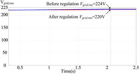
FIGURE 11. When the grid voltage per unit value is between 1 and 1.03 p.u., the unregulated grid voltage value Vgrid and the regulated grid voltage value Vgrid.
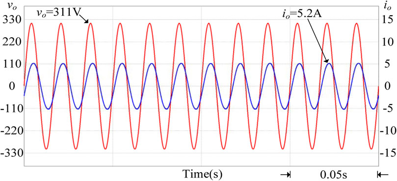
FIGURE 12. When the grid voltage per unit value is between 1 and 1.03 p.u., the output voltage and current waveforms of the smart inverter.
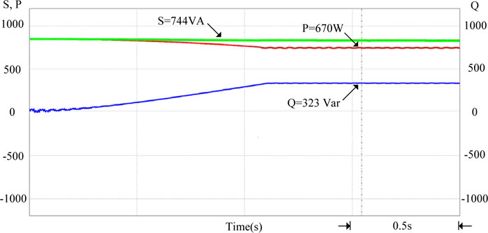
FIGURE 13. When the grid voltage per unit value is between 1 and 1.03 p.u., the active output power and reactive power control situation of the smart inverter.
4.2.3 The Per Unit Value of the Grid Voltage Is Between 0.97 and 1 p.u.
When the photovoltaic power generation system generates a drop in power generation due to building shading or climate, the grid-connected point voltage will be lower than 1 p.u. This will cause electrical loads and small power plants to be damaged, so the grid voltage must be increased. Therefore, when it is detected that the grid voltage per unit value is between 0.97 and 1 p.u., the smart photovoltaic inverter should start to control its output power. In Figure 14, when the PV power injected into the grid is reduced, if the grid voltage value Vgrid1 is not regulated, the voltage value will gradually drop. If the above-mentioned smart photovoltaic inverter voltage-power control is used, the regulated grid voltage value Vgrid2 will rise to an effective value of 220 V (1 p.u.). It can effectively suppress the drop of the grid voltage, and at this time, the output power factor of the smart inverter is 0.9 (leading), supplying reactive power to the grid. Figure 15 shows the output voltage and current waveforms of the smart inverter when the grid voltage per unit value is between 0.97 and 1 p.u. It can be observed from the figure that the current phase leads voltage, so the power factor is leading. Figure 16 shows the output power regulation of the smart inverter when the grid voltage per unit value is between 0.97 and 1 p.u. It can be observed from the figure that the system provides reactive grid power of 323 Var (Q < 0) at this time, and the overall apparent power S still maintains the output power of the photovoltaic module of 744 VA. In contrast, the active output power P of the smart inverter drops to 670 W.
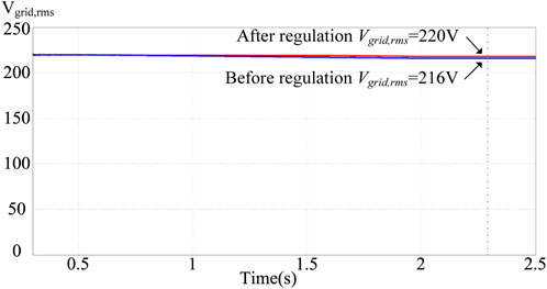
FIGURE 14. When the grid voltage per unit value is between 0.97 and 1 p.u., the grid voltage value Vgrid without regulation and the grid voltage value Vgrid after regulation.
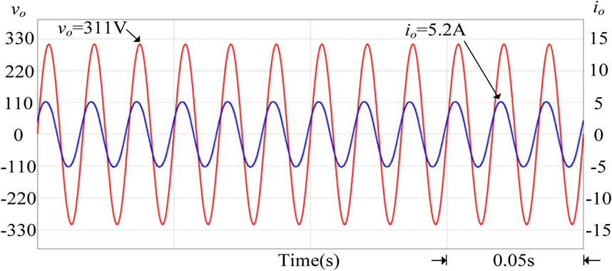
FIGURE 15. When the grid voltage per unit value is between 0.97 and 1 p.u., the output voltage and current of the smart inverter.
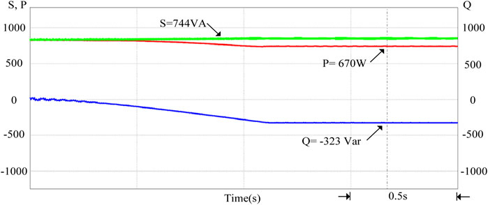
FIGURE 16. The output power control situation of the smart inverter when the grid voltage per unit value is between 0.97 and 1 p.u.
5 Experimental Results
In order to verify the feasibility of simulation results, this study uses the circuit and control system multi-function simulation software PLECS system developed by Swiss company Plexim GmbH. It, along with RT Box and Analog Breakout Broad, has been used to complete the smart inverter test. At the same time, in order to bring out the effectiveness of the voltage-power control of the smart inverter, the PVMAs test capacity is enhanced to 1200 W during implementation. Therefore, the capacity differs from the 744 W adopted in the simulation.
When there are no exceptional changes in the voltage of the PV grid-connected system, the photovoltaic inverter generally controls its output voltage and current in sine waves and in the same phase, so its PF is 1.0. Therefore, the photovoltaic power generation system’s output power is parallel connected to the grid through active power. However, when there is a drastic increase or decrease in the amount of sunlight, the grid-connected photovoltaic power generation system’s power injected into the grid-connected system also increases or decreases drastically. If the load is unable to consume or replenish the increased or decreased electricity drastically, the voltage at the grid-connected point will drastically rise or drop, which may easily cause damage to equipment on the load side. In order to prevent such occurrences, this study uses the smart inverter to adjust effective power and reactive power to stabilize the voltage at the grid-connected point.
When the voltage per unit value of the grid-connected point is between 1.0 and 1.03 p.u., it means the grid system’s reactive power is a negative value (Q < 0), and the power factor of the grid system is leading. Therefore, the output current of the smart inverter must be controlled to lagging voltage to make the power factor lagging and absorb the reactive power of the grid system, thereby stabilizing the voltage at the grid-connected point. Figure 17 implements smart inverter output voltage, and the current waveform shows that when the voltage per unit value of the grid-connected point is between 1.0 and 1.03 p.u., the smart inverter will start controlling the output current to be lagging the output voltage. The power factor is regulated to lagging in order to absorb the reactive power of the system. Figure 18 shows the output power regulation of the smart inverter. It shows that the power regulation of the smart inverter reduces the active power of the inverter grid from 1200 to 1080 W. In addition, the 523 Var (Q > 0) reactive power of the grid system is absorbed by the smart inverter. The total output apparent power is maintained at the PVMA capacity of 1200 VA.
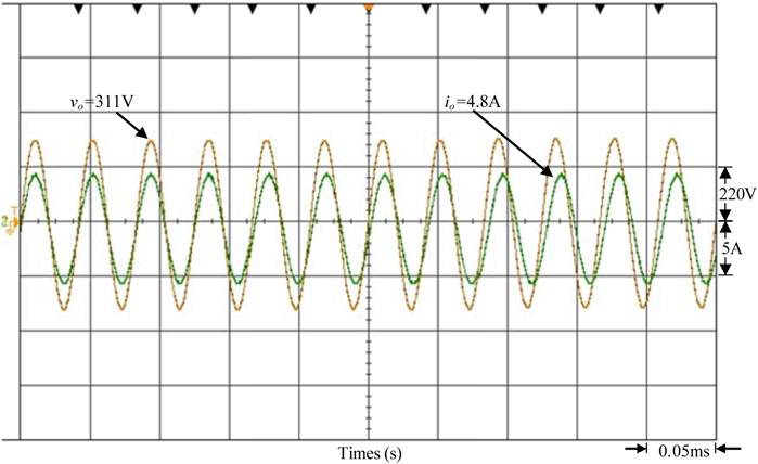
FIGURE 17. The measured output voltage and current of the smart inverter when the grid voltage per unit value is between 1.0 and 1.03 p.u.
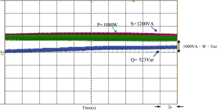
FIGURE 18. The measured output power regulation of the smart inverter when the grid voltage per unit value is between 1.0 and 1.03 p.u.
On the contrary, when the photovoltaic power generation system causes the power generation to drop due to unexpected climate factors such as overcast by dark clouds and other climate factors, this causes the power generation to drop suddenly. When the voltage per unit value of the grid-connected point is between 0.97 and 1.0 p.u., the reactive power of the grid system is a positive value (Q > 0), so the grid system power factor is lagging. Therefore, the output current leading output voltage of the smart inverter must be controlled, so the power factor is leading. Reactive power of the grid system is provided to stabilize the voltage of the grid-connected point by the smart inverter. In Figure 19, the output voltage and current waveforms of the smart inverter show that when the voltage per unit value of the grid-connected point is between 0.97 and 1.0 p.u., the smart inverter begins to control the output current to be leading the output voltage. The power factor is adjusted into leading in order to provide reactive power for the grid system. In Figure 20, the changes in the output power of the smart inverter show that the power regulation of the smart inverter makes the inverter’s active power injected into the gird maintained at 1080 W. However, reactive power 523 Var (Q < 0) is provided to the grid system. The apparent power of the total output is still maintained at 1200 VA capacity for the PVMA.
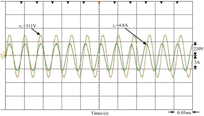
FIGURE 19. The measured waveform of the output voltage and current of the smart inverter when the grid voltage per unit value is between 0.97 and 1.0 p.u.
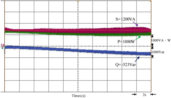
FIGURE 20. The measured output power regulation of the smart inverter when the grid voltage per unit value is between 0.97 and 1.0 p.u.
Through the test and simulation results, it can be verified that the smart photovoltaic inverter developed can provide reactive power to the grid system or absorb reactive power by controlling the power factor at the output end. This will achieve stable grid system voltage. Therefore, the smart inverter developed in this study has been proven to be feasible.
6 Conclusion
This study discusses the design of a grid-connected smart photovoltaic inverter. Its circuit architecture is composed of a boost converter and a single-phase full-bridge inverter and uses SANYO HIP-186BA19 photovoltaic modules. A 744 W photovoltaic module array is formed to perform its maximum power tracking simulation with the extension method under different amounts of sunlight. The simulation results show that the extension method can quickly track the maximum power point under different sunlight conditions. Finally, the tracking results are compared with the traditional perturb and observe method, proving that the extension maximum power tracking method is better in tracking speed and steady-state performance. In the photovoltaic grid-connected inverter control part, this study uses a proportional-integral (PI) controller to control the DC-link voltage at 400 V. The AC output voltage is controlled at an effective value of 220 V. The simulation results prove the photovoltaic power generation system designed in this study. The inverter can indeed be operated in parallel with the grid power operation mode. With the maximum power tracker, the electricity generated by the photovoltaic module array can be smoothly connected to the grid. In addition, when the photovoltaic module array is affected by factors such as sunlight changes and shading, resulting in unstable power generation, this study uses the voltage-power controller in the photovoltaic grid-connected inverter to control the output of the smart inverter. The amount of active and reactive power enables the grid voltage to be maintained within the specified range, thereby improving the power quality of the grid system.
Data Availability Statement
The original contributions presented in the study are included in the article/supplementary material. Further inquiries can be directed to the corresponding author.
Author Contributions
K-HH proposed the voltage-power control conceptualization of the photovoltaic grid-connected inverter. K-HC provided the conceptualization of maximum power point tracking for the photovoltaic power generation system and completed the formal analysis of the tracking algorithm based on the extension theory. K-HC was in charge of project administration. K-HH and K-HC were also responsible for the writing, review, and editing of this paper. Z-YS completed the simulation and experimental results of voltage-power control of the smart photovoltaic grid-connected inverter to improve the power quality of the grid system. Y-HL carried out the data curation, software program, and simulation validation for the proposed maximum power point tracking controller. All of the authors have read and agreed to the published version of the manuscript.
Funding
This study was financially supported by the Ministry of Science and Technology of Taiwan under Grant no. MOST 110-2221-E-167-007-MY2.
Conflict of Interest
The authors declare that the research was conducted in the absence of any commercial or financial relationships that could be construed as a potential conflict of interest.
Publisher’s Note
All claims expressed in this article are solely those of the authors and do not necessarily represent those of their affiliated organizations or those of the publisher, the editors, and the reviewers. Any product that may be evaluated in this article, or claim that may be made by its manufacturer, is not guaranteed or endorsed by the publisher.
References
Azab, M. (2017). “Flexible PQ Control for Single-phase Grid-Tied Photovoltaic Inverter,” in IEEE International Conference on Environment and Electrical Engineering and IEEE Industrial and Commercial Power Systems Europe, June 13, 2017. doi:10.1109/EEEIC.2017.7977550
Bing, X., Youwei, Z., Xueyan, Z., and Xuekai, S. (2021). “An Improved Artificial Bee Colony Algorithm Based on Faster Convergence,” in 2021 IEEE International Conference on Artificial Intelligence and Computer Applications, June 28-30, 2021. doi:10.1109/ICAICA52286.2021.9498254
Bletterie, B., Bründlinger, R., and Lauss, G. (2010). On the Characterisation of PV Inverters' Efficiency-Introduction to the Concept of Achievable Efficiency. Prog. Photovolt. Res. Appl. 19 (4), 423–435. doi:10.1002/pip.1054
Chao, K.-H., and Li, C.-J. (2010). An Intelligent Maximum Power Point Tracking Method Based on Extension Theory for PV Systems. Expert Syst. Appl. 37 (2), 1050–1055. doi:10.1016/j.eswa.2009.06.068
Chao, K.-H., Wang, M.-H., and Lee, Y.-H. (2011). “An Extension Neural Network Based Incremental MPPT Method for a PV System,” in 2011 International Conference on Machine Learning and Cybernetics, July 10-13, 2011. doi:10.1109/ICMLC.2011.6016761
Chao, K. H., Huang, C. H., and Chang, Y. C. (2012). “Design and Implementation of a Photovoltaic System for an Air Conditioner,” in Proceedings of Seventh Intelligent Living Technology Conference, 2012.
Chao, K. H., and Lee, Y. H. (2011). An Intelligent Incremental Conductance MPPT Method for a Photovoltaic System. Key Engin. Mater. 480-481, 739–744. doi:10.4028/KEM.480-481.73910.4028/www.scientific.net/kem.480-481.739
Chen, W. L., and Chien, M. C. (2014). Design and Control of Grid-Tied Single Phase Inverters. Dissertation/Master’s Thesis (Taoyuan City (GD): Chang Gung University, Taiwan).
Ciobotaru, M., Teodorescu, R., and Blaabjerg, F. (2005). “Control of Single-Stage Single-Phase PV Inverter,” in 2005 European Conference on Power Electronics and Applications, Sept. 11-14, 2005. doi:10.1109/EPE.2005.219501
Fan Yang, F., and Caili Zhang, C. (2011). “A Classification Model Based on Extenics with Weighted Features for Rolling Bearing Quality Test,” in 2011 Second International Conference on Mechanic Automation and Control Engineering, July 15-17, 2011. doi:10.1109/MACE.2011.5987814
He, F., Zhao, Z., Yuan, L., and Lu, S. (2011). “A DC-Link Voltage Control Scheme for Single-Phase Grid-Connected PV Inverters,” in 2011 IEEE Energy Conversion Congress and Exposition, Sept. 17-22, 2011. doi:10.1109/ECCE.2011.6064305
Krause, P. C., wasynczuk, O., and Sudhoff, S. D. (2002). Analysis of Electric Machinery and Drive Systems. Second Edition. Piscataway Township: Wiley-IEEE Press.
Li, Y., Ang, K. H., and Chong, G. C. Y. (2006). Patents, Software, and Hardware for PID Control: An Overview and Analysis of the Current Art. IEEE Control Syst. 26 (1), 42–54. doi:10.1109/MCS.2006.1580153
Pearsall, N. (2017). The Performance of Photovoltaic (PV) Systems : Modelling, Measurement and Assessment. Amsterdam: Elsevier Press.
Pragallapati, N., Sen, T., and Agarwal, V. (2017). Adaptive Velocity PSO for Global Maximum Power Control of a PV Array Under Nonuniform Irradiation Conditions. IEEE J. Photovoltaics 7 (2), 624–639. doi:10.1109/JPHOTOV.2016.2629844
PSIM Website (2022). PSIM. Available at: https://powersimtech.com/products/psim/ (Accessed February 16, 2022).
SANYO HIP-186BA19 Data Sheet (2014). Data Sheet. Available at: https://www.energymatters.com.au/images/Sanyo/Sanyo20190W.pdf (Accessed July 15, 2014).
Saoji, A., and Rao, G. S. (2021). “Hybrid [ACPSO] Integration Approach Based on Particle Swarm Optimization and Ant Colony Optimization to Improve Lifetime of Wireless Sensor Network,” in 2021 Asian Conference on Innovation in Technology, Aug. 27-29, 2021. doi:10.1109/ASIANCON51346.2021.9544535
Sen, T., Pragallapati, N., Agarwal, V., and Kumar, R. (2018). Global Maximum Power Point Tracking of PV Arrays Under Partial Shading Conditions Using a Modified Particle Velocity‐Based PSO Technique. IET Renew. Power Gener. 12 (5), 555–564. doi:10.1049/iet-rpg.2016.0838
Urakabe, T., Fujiwara, K., Kawakami, T., and Nishio, N. (2010). “High Efficiency Power Conditioner for Photovoltaic Power Generation System,” in The 2010 International Power Electronics Conference - ECCE ASIA, June 21-24, 2010. doi:10.1109/IPEC.2010.5543123
Usher, E., and Martel, S. (1994). “Avoided Cost Benefits of PV on Diesel-Electric Grids,” in Proceedings of 1994 IEEE 1st World Conference on Photovoltaic Energy Conversion - WCPEC (A Joint Conference of PVSC, PVSEC and PSEC), Dec. 5-9, 1994. doi:10.1109/WCPEC.1994.520141
Keywords: photovoltaic power generation system, maximum power tracking, extension theory, smart inverter and PV system control, power quality
Citation: Huang K-H, Chao K-H, Sun Z-Y and Liao Y-H (2022) Online Control of Smart Inverter for Photovoltaic Power Generation Systems in a Smart Grid. Front. Energy Res. 10:879385. doi: 10.3389/fenrg.2022.879385
Received: 19 February 2022; Accepted: 25 May 2022;
Published: 19 July 2022.
Edited by:
Chengzong Pang, Wichita State University, United StatesReviewed by:
Mohamed Salem, Universiti Sains Malaysia (USM), MalaysiaRazman Ayop, University of Technology Malaysia, Malaysia
Copyright © 2022 Huang, Chao, Sun and Liao. This is an open-access article distributed under the terms of the Creative Commons Attribution License (CC BY). The use, distribution or reproduction in other forums is permitted, provided the original author(s) and the copyright owner(s) are credited and that the original publication in this journal is cited, in accordance with accepted academic practice. No use, distribution or reproduction is permitted which does not comply with these terms.
*Correspondence: Kuei-Hsiang Chao, Y2hhb2toQG5jdXQuZWR1LnR3