A Positive Climatic Trend in the Global Offshore Wind Power

The climatic variation of offshore wind energy has a close relationship with the long-term plan of energy utilization. However, the work on this aspect is scarce and mainly focuses on the variation of wind power density (WPD). There is little research on the climatic trends of effective wind speed occurrence (EWSO) and occurrence of energy level greater than 200 W/m² (rich level occurrence, RLO), which are directly related to the available rate and richness of wind energy. Based on the ERA-Interim wind product from the ECMWF, this study calculated the climatic trends of series of key factors of wind energy in the global oceans, including the WPD, EWSO, and RLO. The results show that the wind energy exhibits a positive trend globally for the past 36 years, with overall annual increasing trends in WPD, EWSO, and RLO, of 0.698 (W/m²)/yr, 0.076%/yr, and 0.090%/yr separately. The annual trend exhibits evident regional differences. The areas with significant increasing trends are mainly distributed in the mid- low-latitude waters of global oceans and part of the southern hemisphere westerlies. The annual increasing trend of WPD is strongest in the southern westerlies, especially in the extratropical South Pacific (ETSP), of about 1.64 (W/m²)/yr. The annual increasing trends of EWSO and RLO are strongest in the tropical waters, especially the tropical Pacific Ocean (TPO), of 0.17%/yr and 0.19%/yr separately. The annual and seasonal WPD, EWSO, and RLO in most global oceans have significant increasing trends or no significant variation, meaning that the wind energy trends are rich or stable, which is beneficial for energy development. The climatic trends of wind energy are dominated by different time periods. There is no evident abrupt change of wind energy in the extratropical waters globally and tropical Atlantic Ocean (TAO). The abrupt periods of wind energy in the TIO and TPO occurred in the end of the 20th century and the beginning of the 21st century. The wind energy of the South China Sea, Arabian Sea, and the Bay of Bengal and nino3 index share a common period of approximately 5 years. The offshore wind energy was controlled by an oscillating phenomenon.

Highlights

• We systematically presented the climatic trends of series of wind energy factors (WPD, EWSO, and RLO).

• A positive climatic trend in the global offshore wind energy was found.

• The climatic trend exhibits obvious regional and seasonal differences.

• The annual increasing trend of WPD is strongest in the southern westerlies.

• The annual increasing trends of EWSO and RLO are strongest in the tropical waters.

• The global offshore wind energy was controlled by an oscillating phenomenon.

Introduction

Given the current background of ongoing environmental and resource issues, the full development and utilization of renewable energy (such as wave energy and offshore wind energy) can effectively alleviate the energy crisis and contribute to emission reduction and environmental protection (Xydis, 2016; Khojasteh et al., 2018; Akpınar et al., 2019), thus promoting the sustainable development of human society and isolated islands. Understanding the energy characteristics is important for the efficient development of wind energy resources.

Studies have been provided by the previous researchers to reveal the spatial distribution of renewable energy resources. Amirinia et al. (2017) presented an analysis on the wind energy of the southern Caspian Sea using uncertainty analysis. They found total exploitable wind energy of 915 GWh in this area. Soares et al. (2020) carried out offshore wind energy resources in global oceans using the new ERA-5 reanalysis. The widespread gains (ranging between +5% and +50%) throughout the global economic exclusive zones and no losses for all seasons. Also, the wind power density is 800 W/m² in the mid- and high latitudes, and higher than 400 W/m² along the Eastern Boundary Current Systems. Wen et al. (2021) analyzed the offshore wind energy of the south and southeast coasts of China using Japanese 55-year reanalysis (JRA-55). The suggested future offshore wind power development is found to be the coasts of Hong Kong. Esteban et al. (2009) designed an integral management applied to offshore wind farms. In this scheme, the territory, terrain, and physical–chemical properties of the contact area between the atmosphere and the ocean were considered, which has an important reference for the wind power plant site selection. Chen et al. (2020) presented an assessment of wind energy of seven sites in the Beibu Gulf using observation data. The results show that the annual mean wind power density at 100 m above mean sea level was, respectively, 605.6, 542.0, 368.0, 282.0, 265.6, 87.6, and 321.5 W/m² at the seven sites. Akpınar et al. (2021) analyzed the spatial characteristics of wind and wave parameters over the Sea of Marmara. They found that the highest mean wind speeds are observed in winter and the lowest in spring. Higgins and Foley (2014) analyzed the offshore wind power in the United Kingdom. They pointed out that the United Kingdom has the potential to continue to lead the world in offshore wind power as it has over 48 GW of offshore wind power projects at different stages of operation and development. Higgins et al. (2014) analyzed the impact of offshore wind power forecast on the electricity cost. Results show that the impact from wind power forecast error can be up to 2000 MW. Devlin et al. (2017) pointed out that gas generation is crucially important to the continued growth of renewable energy. Bosch et al. (2018) pointed out that 64,845 TWh is available globally in shallow waters (0–40 m), while 103,852 TWh is located within 10–50 km of the coastline globally using global wind speeds from the National Aeronautics and Space Administration (NASA) Modern-Era Retrospective analysis for Research and Applications, version 2 (MERRA-2) reanalysis data set. Liu et al. (2017) found a significant increasing trend in gale days in the South China Sea and North Indian Ocean for 1988–2011, using CCMP wind data. The area with a strong increasing trend is located in the Taiwan Strait, Luzon Strait, and the Indo-China Peninsula waters. Capps and Zender (2009) calculated the 80 m wind power in global oceans using satellite observation data. They pointed out that the 80 m wind power is 1.2–1.5 times 10 m power equatorward of 30 latitude, 1.4–1.7 times 10 m power in wintertime storm track regions, and above 6 times 10 m power in stable regimes east of continents. Young et al. (2011) found a general global increasing wind speed (WS) trend for the period 1991–2008, utilizing an 18-year database of calibrated and validated satellite altimeter measurements. Thomas et al. (2008) pointed out that for the period 1982–2002, the WS trend remained within the annual mean for spatially averaged adjusted winds, 4 (cm/s)/yr for estimated speeds and 2 cm s⁻¹ yr⁻¹ for measured speeds, over most of the global oceans.

There are many research studies on the long-term trends of meteorological and marine elements. However, the research on the climatic trend of wind energy is scarce, although it is one of the most important points to consider in wind power plant site selection and long-term planning. Zheng et al. (2017) presented the recent decadal trend in wind power density (WPD) of the North Atlantic, and they pointed out that the North Atlantic WPD exhibited a significant increasing trend of 4.45 (W/m²)/yr for the period 1988–2011. Jiang et al. (2019) calculated the trends of sea surface wind energy over the South China Sea using 24-year Cross-Calibrated Multi-Platform (CCMP) wind data. The trend was greatest in winter, followed by spring, and smallest in summer and autumn. As a whole, the existing research is mainly focused on the variation of WPD. The analysis on the climatic variations of the energy availability and richness is almost blank, although they are closely related to the wind energy utilization. In the actual development of wind energy, the long-term planning of wind energy schemes is concerned not only with the climatic trend of the WPD but also with the trends of the EWSO and occurrence of the energy level greater than 200 W/m² (rich level occurrence, RLO) that directly determined the wind energy utilization rate and energy richness. This study comprehensively calculated the long-term trends of the aforementioned key factors globally, in hope of providing reference for the long-term plan of wind energy utilization and analysis of global climate change.

Methodology and Data

Data

The ERA-Interim wind data are hosted at the European Centre for Medium-Range Weather Forecasts (ECMWF), which is a new production after the ERA-40. There also exists a great improvement in the assimilation method and application of observation data. Its time resolution is 6 hourly intervals. The spatial resolution covers 0.125° × 0.125°, 0.25° × 0.25°, 0.5° × 0.5°,..., 2.5° × 2.5°. In this study, the spatial resolution of 0.25° × 0.25 ° is used. It covers the time range from January 1979 to December 2014 and a space range of 90°S–90°N and 0.0°E–359.875°E. The ERA-Interim wind data are proved to have a high precision than the observation data (Dee et al., 2011; Song et al., 2015) and can be available at https://apps.ecmwf.int/datasets/data/interim-full-daily/levtype=sfc/ (European Centre for Mediu, 2011).

Methods

Generally, the WS of 5–25 m/s is suitable for wind energy utilization (Miao et al., 2012), which was regarded as effective WS. Obviously, the EWSO is directly related to the wind energy utilization rate. Usually, wind energy with a WPD greater than 200 W/m² is considered to be abundant. Zheng et al. (2013) defined the occurrence of energy levels greater than 200 W/m² as rich level occurrence (RLO). As a result, this study presented the climatic trends of series of key factors of wind energy, comprehensively including the WPD, EWSO, and RLO, to provide scientific reference for the long-term planning of wind energy development and analysis on the global climatic change.

First, the 6-hourly global offshore WPD of 10 m above the sea surface at each 0.25° × 0.25° grid point for the period 1979.01–2014.12 is obtained based on the ERA-Interim wind product and calculation method for WPD (Capps and Zender, 2010). Based on the 6-hourly WS data and WPD data, the EWSO and RLO at each 0.25° × 0.25° grid point of each month for the period 1979.01–2014.12 are counted separately. Then, the spatial–temporal distributions of WPD, EWSO, and RLO were exhibited.

Second, the climatic trend of global offshore wind energy resource was calculated, systematically including the overall annual trend, regional difference of the annual trend, seasonal difference of the trend, dominant season of the trend, and the trends of key regions in different months. Using the linear regression method, the overall annual trends of global WPD, EWSO, and RLO for the past 36 years (1979–2014) are calculated. In order to exhibit the regional difference of the climatic trend, the annual trend of WPD at each 0.25° × 0.25° grid point is calculated. Similarly, the regional differences of the annual trends in EWSO and RLO are also calculated separately. To reveal the seasonal difference of the trend, the trends of WPD, EWSO, and RLO at each 0.25° × 0.25° grid point in MAM (March-April-May), JJA (June-July-August), SON (September-October-November), and DJF (December-January-February) are calculated separately, and the dominant season of the trend was also presented.

In addition, the Mann–Kendall (M-K) test and wavelet analysis methods were employed to calculate the abrupt change and variation period of wind energy in the global oceans separately. At last, an analysis on the relationship between the wind energy and key oscillating phenomenon in the global oceans was also carried out, to reveal the mechanism of the climatic variation of wind energy.

The calculation methods of WPD, RLO, and EWSO are as follows:

$WPD=\frac{1}{2}\rho V^3,(1)$

$EWSO=\frac{t_1}{T}\times 100\%,(2)$

$RLO=\frac{t_2}{T}\times 100\%,(3)$

where WPD is the wind power density (unit: W/m²), V is the wind speed (unit: m/s), and $\rho$ is the surface air density (unit: kg/m³), while the last one is usually 1.225 kg/m³ under standard conditions for temperature and pressure with an altitude below 500 m (Capps and Zender, 2010). EWSO is the effective wind speed occurrence (unit: %), and t₁ is the number of time steps with wind speed between 5 and 25 m/s. RLO is the rich level occurrence (unit: %), and t₂ represents the time steps with WPD greater than 200 W/m². T represents the total number of time steps analyzed.

The Thiessen polygon method was as follows:

$\overline{R}=\frac{{\displaystyle \sum _{\text{i}=1}^i{\text{A}}_i{R}_i}}{{\displaystyle \sum _{\text{i}=1}^i{\text{A}}_i}},(4)$

where A_i is the area of each Thiessen polygon and R_i is the value of WPD at each grid point. The Thiessen polygon method mainly includes the following steps: 1) draw lines joining adjacent gages, 2) draw perpendicular bisectors to the lines created in the first step, 3) extend the lines created in the second step in both directions to form representative areas for gages, 4) compute the representative area of each gage, and 5) compute the areal average using formula 4.

The M-K test method was as follows. Construct a rank series for a time series x with n sample size as follows (Wang, 2020):

${\text{S}}_{\text{k}}={\displaystyle \sum _{\text{i}=1}^{\text{k}}{\displaystyle \sum _{\text{j}}^{\text{i}-1}{\text{a}}_{\text{i}\text{j}}\left(\text{k}=\mathrm{2,3,4},\dots \text{n}\right)}}.(5)$

${\text{a}}_{\text{ij}}=\{\begin{array}{l}1\left(X_i>X_j\right)\\ 0\left(X_i<X_j\right)\end{array}\sqrt{a^2+b^2}\left(1\le \mathrm{j}\le \mathrm{i}\right).(6)$

Define the following statistics under the hypothesis that the time series x is randomly independent as follows:

$U{F}_{\text{k}}=\frac{\left[S_k-E\left(S_k\right)\right]}{\sqrt{Var\left(S_k\right)}}\left(K=\mathrm{1,2,3,4},\dots ,\mathrm{n}\right),(7)$

$E\left(S_{\text{k}}\right)=k(K+1/4);V_{ar}\left(S_{\text{k}}\right)=k(k-1)(2k+5)/72,(8)$

$\{\begin{array}{l}U{B}_k=-U{F}_k\\ k=n+1-k\end{array}\left(K=\mathrm{1,2,3,4},\dots ,\mathrm{n}\right),(9)$

where UF₁ = 0, ans E (S_k) and Var(S_k) are the average value and variance of S_k, respectively. UF_i abides by the standard normal distribution, which is a sequence of statistics calculated in time series x order x₁, x₂,…, x_n.

Results

Spatial–Temporal Distribution of Wind Power Density, Effective Wind Speed Occurrence, and Rich Level Occurrence

Averaging the WPD from 1979.01.01 to 2014.12.31, the multi-year average WPD at each 0.25° × 0.25° grid point globally is obtained, as shown in Figure 1A. The large areas of WPD are mainly distributed in the southern hemisphere westerlies (>800 W/m²) and the northern hemisphere westerlies (>600 W/m²). The relative indigent areas are small and mainly distributed in the low-latitude waters (<200 W/m²). Wind energy resources with a WPD greater than 200 W/m² are generally considered to be abundant. Obviously, most of the global oceans are rich in wind energy resources. Zheng and Pan (2014) calculated the global offshore WPD using 24-year CCMP wind data. The results show that the large areas of wind energy density are mainly distributed in westerlies, of above 800 W/m² in the southern hemisphere westerlies and above 600 W/m² in the northern hemisphere westerlies. The area scope with WPD greater than 1,200 W/m² in the southern hemisphere westerlies of this study is slightly larger than that of Zheng and Pan (2014), while the area scope with WPD greater than 1000 W/m² in the North Atlantic Ocean westerly of this study is smaller than that of Zheng and Pan (2014) and Liu et al. (2008). Guo et al. (2018) analyzed the global offshore wind energy using scatterometers (QuikSCAT, ASCAT) and radiometers (WindSAT). Both the area scopes with WPD greater than 1,200 W/m² in the southern hemisphere westerlies and area scope with WPD greater than 1,000 W/m² in the northern hemisphere westerlies obtained by Guo et al. (2018) are larger than that of this study. As a whole, there is consistency between this study and Zheng and Pan (2014), Liu et al. (2008) and Guo et al. (2018).

FIGURE 1

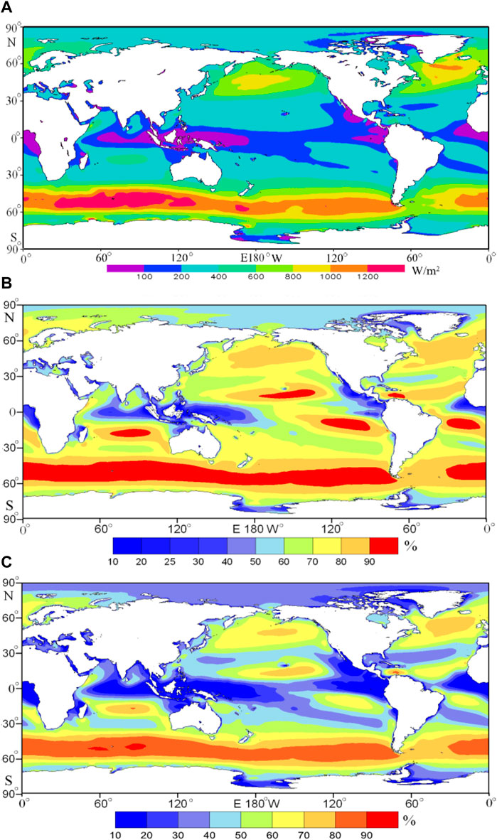
FIGURE 1. Multi-year average wind power density (A), effective wind speed occurrence (B), and rich level occurrence (C) in the global oceans.

The EWSO and RLO in each month for the period 1979.01–2014.12 are counted separately, based on the 6-hourly WS data and WPD data. Then, the multi-year average EWSO and RLO at each 0.25° × 0.25° grid point are obtained, by averaging the EWSO and RLO from 1979.01 to 2014.12 separately, as shown in Figures 1B,C. Obviously, the EWSO is optimistic, of >60% in most of the global oceans. The southern and the northern hemisphere westerlies are the large regions. It is worth noting that there exist several large areas of EWSO in the mid-low-latitude waters of global oceans (even >90% in the large center), meaning an optimistic wind energy utilization rate although they are not distributed in the large area of WPD. The spatial distribution feature of the RLO is similar to that of EWSO.

Overall Trends of the Global Oceanic Wind Power Density, Effective Wind Speed Occurrence, and Rich Level Occurrence

Averaging the WPD from 0000 UTC on 1 January 1979 to 1800 UTC on 31 December 1979, an annual mean value of WPD at each 0.25° × 0.25° grid point is obtained. Then, a zonal average value of WPD for global oceans in 1979 was obtained using the Thiessen polygon method. Using the same method, zonal and annual mean values of WPD for global oceans for the period 1979–2014 were obtained. Then, the overall trend of the global oceanic WPD is calculated using the linear regression method, as shown in Figure 2A. Similarly, the overall trends of WPD in the south global ocean and the north global ocean were also obtained, as shown in Figures 2B,C.

FIGURE 2

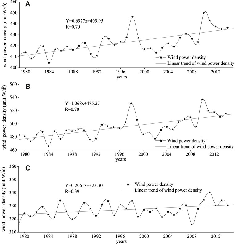
FIGURE 2. Annual average wind power density in the global ocean (A), south global ocean (B), and the north global ocean (C) for the period 1979–2014 and the long-term trends.

As shown in Figure 2A, the correlation coefficient (R) of the WPD is 0.70, significant at the 0.001 level test (|R| = 0.70 > r_0.001 = 0.51). The regression coefficient is 0.698. It means that the WPD exhibits a significant increasing trend of 0.698 (W/m²)/yr in the global ocean as a whole for the period 1979–2014. Similarly, the WPD in the south global ocean has a significant increasing trend of 1.068 (W/m²)/yr (significant at the 0.001 level). The WPD in the north global ocean has a significant overall increasing trend, of 0.206 (W/m²)/yr (significant at the 0.05 level). It is not hard to find that the WPD curve of the global ocean is similar to that of the south global ocean, while there is an obvious difference between the WPD curve of the global ocean and that of the north global ocean, meaning that the variation of the WPD in the global ocean is mainly dominated by the south global ocean.

Based on the 6-hourly WS data from 0000 UTC on 1 January 1979 to 1800 UTC on 31 December 1979, the EWSO at each 0.25° × 0.25° grid point for global oceans in 1979 is counted. Then a zonal average value of EWSO for global oceans was obtained using the Thiessen polygon method. Similarly, 36 zonal and yearly mean values of EWSO were obtained. Then, the overall variation of the global EWSO is exhibited using the linear regression method, as shown in Figure 3A. Similarly, the overall variation of EWSO in the south global ocean and north global ocean was also presented separately, as shown in Figures 3B,C. Obviously, the EWSO in the global ocean, south global ocean, and north global ocean has significant increasing trends (significant at the 0.001 level) of 0.076, 0.080, and 0.071%/yr separately (here, % is the EWSO, not the variation rate of EWSO, same as follows). It is also worth noting that the EWSOs in the global ocean, south global ocean, and north global ocean are optimistic, of above 60%. It is not hard to find that the EWSO of the global ocean is dominated by the south global ocean.

FIGURE 3

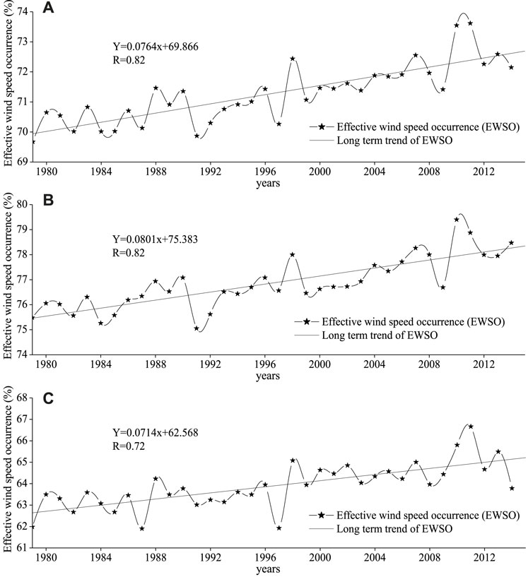
FIGURE 3. Annual effective wind speed occurrence in the global ocean (A), south global ocean (B), and the north global ocean (C) for the period 1979–2014 and the long-term trends.

Based on the 6-hourly WPD data from 0000 UTC on 1 January 1979 to 1800 UTC on 31 December 1979, the RLO at each 0.25° × 0.25° grid point for global oceans in 1979 is counted. Then, a zonal average value of RLO for the global oceans was obtained. Similarly, 36 zonal and yearly mean values of RLO were obtained. Then, the overall variation of the global RLO is exhibited using the linear regression method, as shown in Figure 4A. Similarly, the overall variation of RLO in the south global ocean and north global ocean was also presented separately, as shown in Figures 4B,C. Obviously, the RLOs in the global ocean, south global ocean, and north global ocean have significant increasing trends (significant at the 0.001 level) for the past 36 years, of 0.090, 0.110, and 0.064%/yr separately (here, % is the RLO, not the variation rate of RLO, same as follows).

FIGURE 4

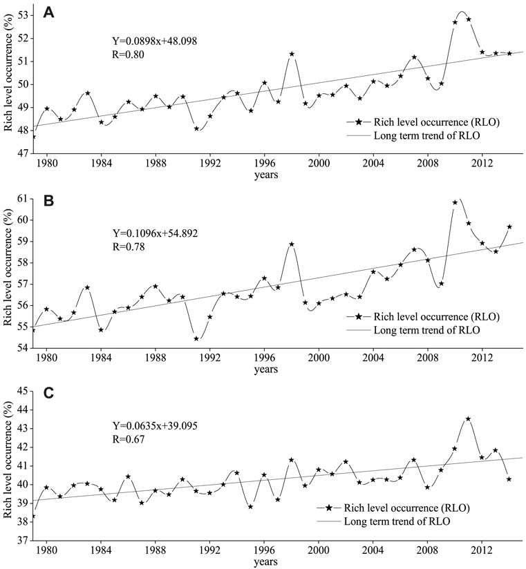
FIGURE 4. Annual rich level occurrence in the global ocean (A), south global ocean (B), and the north global ocean (C) for the period 1979–2014 and the long-term trends.

Regional Differences of the Climatic Trends in the Wind Power Density, Effective Wind Speed Occurrence, and Rich Level Occurrence

Figure 2 presents the overall trend of the WPD in the global ocean. To exhibit the regional difference, the annual trend of WPD at each 0.25° × 0.25° grid point is calculated, as shown in Figure 5A. The areas with significant increasing trends in WPD are mainly distributed in the Somali waters of 1–3 (W/m²)/yr, equator waters of the south Indian Ocean of 0–2 (W/m²)/yr, the mid-low latitude of the mid-east of the Pacific Ocean of 0–4 (W/m²)/yr, the low latitude of the South Atlantic Ocean of 0–2 (W/m²)/yr, and about half of the southern hemisphere westerlies of 3–6 (W/m²)/yr. The area range with a significant decreasing trend is small and mainly located in the south and southeast coast of Greenland and the middle of the North Pacific Ocean westerly. Zheng et al. (2017) found a significant increasing trend of WPD in the southeast coast of Greenland. Earl et al. (1980–2010) found a decreasing trend in WPD, of −3 (W/m²)/yr, in the United Kingdom for 1980–2010, using data from a 40-station wind monitoring network. This study is consistent with the results of Earl et al. (1980–2010) and different from Zheng et al. (2017).

FIGURE 5

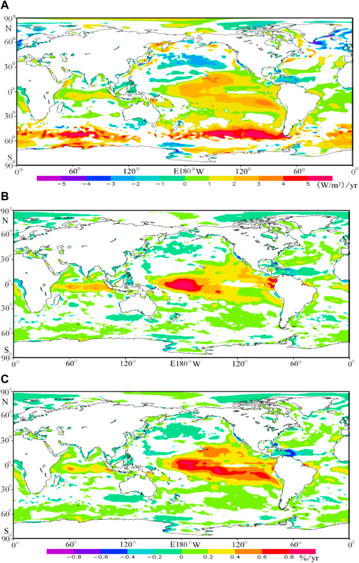
FIGURE 5. Annual climatic trends of the wind power density (A), effective wind speed occurrence (B), and rich level occurrence (C) in the global ocean. Only area significant at 95% level is presented.

The annual trends of EWSO at each 0.25° × 0.25° grid point are presented in Figure 5B. First, the EWSO at each 0.25° × 0.25° grid point for the year 1979 is counted, using the 6-hourly WS data. Similarly, the EWSO of each year at each 0.25° × 0.25° grid point for the period 1979–2014 is counted. Then, the annual trend of EWSO at each 0.25° × 0.25° grid point is calculated. The areas with significant increasing trends in EWSO are mainly distributed in the equator waters of the south Indian Ocean (of 0–0.6%/yr, here % is the EWSO, not the variation rate of EWSO, same as follows), the mid-low latitude of the Pacific Ocean (0.2–1.0%/yr), and some small regions. The area range with significant decreasing trends is small and mainly located in the low latitude of the North Atlantic Ocean and the north pole, of −0.2∼0%/yr.

The same method in Figure 5B is used to calculate the annual trends of RLO at each 0.25° × 0.25° grid point, as shown in Figure 5C. The areas with a significant increasing trend in RLO are mainly distributed in the low-latitude waters of the Indian Ocean and the mid-low-latitude waters of the Pacific Ocean, even up to 0.8%/yr (here % is the RLO, not the variation rate of RLO, same as follows) in the large center. The areas with a significant decreasing trend are distributed in the low-latitude waters of the mid-east of the North Atlantic Ocean, the mid-west of the North Pacific Ocean westerly, and the North Pole.

Seasonal Differences of the Climatic Trends in the Wind Power Density, Effective Wind Speed Occurrence, and Rich Level Occurrence

To reveal the seasonal difference of the trend in the WPD, the method in Figure 5A is employed to calculate the trends of WPD in MAM, JJA, SON, and DJF, as shown in Figure 6. Irrespective of the season, the WPD in most of the global oceans has a significant increasing trend or no significant variation, while only some small regions have a significant decreasing trend, which is an optimistic trend (to be rich or stable) for wind energy development. Comparing Figure 6 with Figure 5A, the annual increasing trend of WPD in the Somali waters is mainly dominated by SON. The increasing trends in the equator of the south Indian Ocean and the mid-low latitude of the Pacific Ocean can be seen in each season. The increasing trend in the south Indian Ocean westerly is dominated by MAM and DJF. The increasing trend in South Pacific Ocean westerly is dominated by MAM, followed by SON. The decreasing trend in the low-latitude waters of the North Atlantic Ocean is dominated by JJA, followed by SON. The decreasing trend in the middle of the North Pacific Ocean westerly is mainly dominated by the MAM, JJA, and SON. Jiang et al. (2019) have found a greater trend of increase in the northern areas of the South China Sea than in southern parts. The result in this study is consistent with Jiang et al. (2019).

FIGURE 6

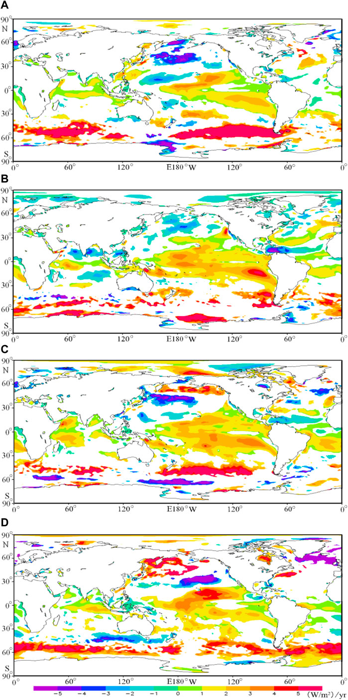
FIGURE 6. Long-term trends of the wind power density in MAM (A), JJA (B), SON (C), and DJF (D) in the global ocean. Only area significant at 95% level is presented.

The method in Figure 5B is used to calculate the trend of EWSO in each season, as shown in Figure 7. The EWSO exhibits no significant variation or a significant increasing trend globally in each season, while only some small regions have a significant decreasing trend, meaning a stable or increasing available rate of wind energy, which is beneficial for the wind energy development. The increasing trend of EWSO in the low-latitude waters of the Indo-Pacific Ocean is much stronger than that in other waters, especially in the mid-west equator of the Pacific Ocean (up to 0.8%/yr in each season). Comparing Figure 7 with Figure 5B, the annual trend of EWSO in different areas is dominated by different seasons. The increasing trends in the equator of the south Indian Ocean and the mid-low latitude of the Pacific Ocean are dominated by MAM and DJF, followed by JJA and SON. The increasing trend in the mid-low latitude of the Pacific Ocean can be clearly seen in each season. The decreasing trend in the low-latitude waters of the North Atlantic Ocean is dominated by JJA and SON.

FIGURE 7

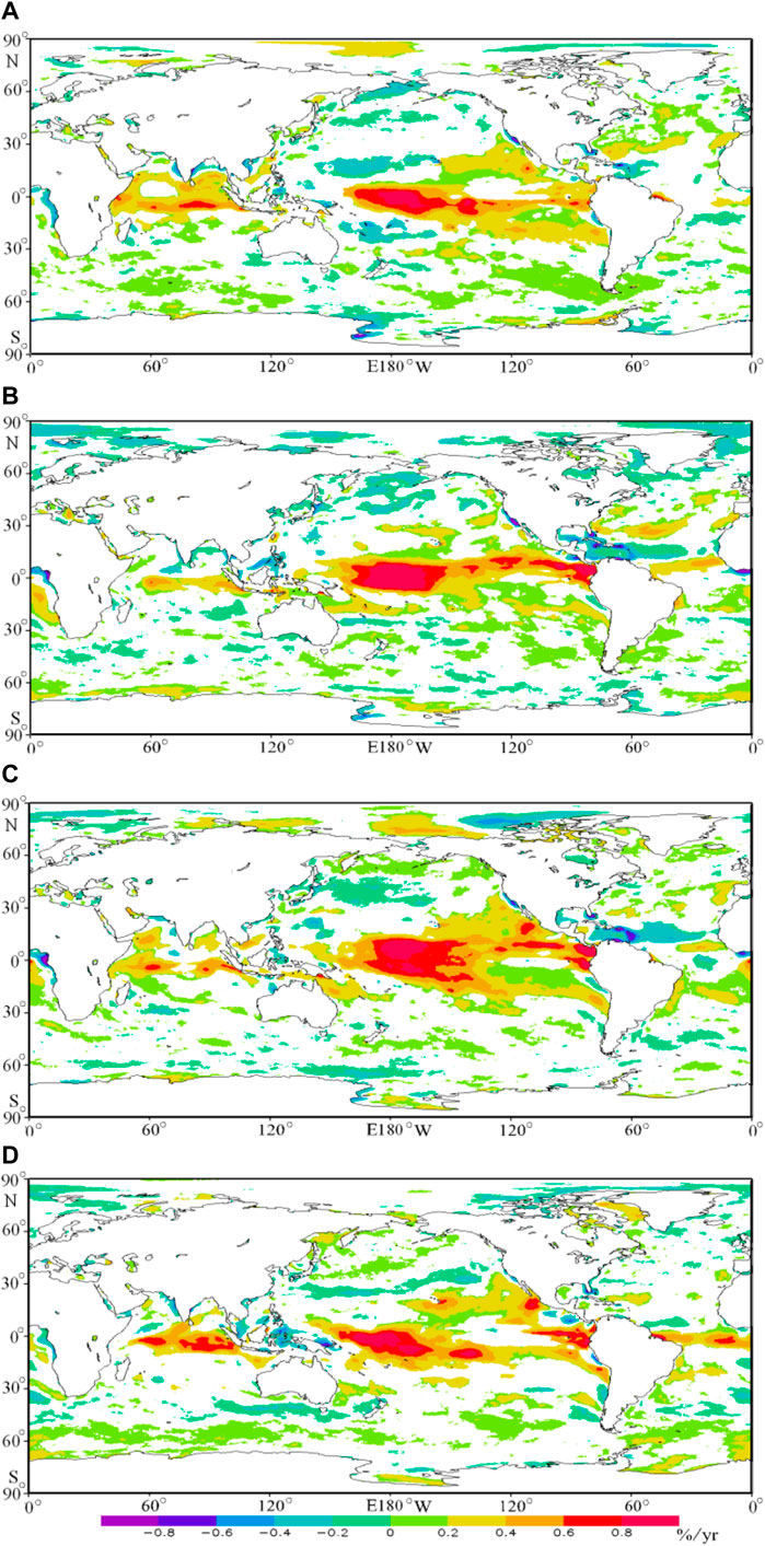
FIGURE 7. Long-term trends of the effective wind speed occurrence in MAM (A), JJA (B), SON (C), and DJF (D) in the global ocean. Only area significant at 95% level is presented.

The method in Figure 5C is used to calculate the trend of RLO in each season, as shown in Figure 8. The RLO in most of the global oceans has no significant variation or a significant increasing trend, meaning a stable or increasing energy-rich rate. Comparing Figure 8 with Figure 5C, the annual increasing trend of EWSO in the Somali waters is dominated by SON, followed by MAM. The annual increasing trends in the equator of the south Indian Ocean and the mid-low latitude of the Pacific Ocean can be reflected in each season. The decreasing trend in the low-latitude waters of the North Atlantic Ocean is dominated by JJA and SON.

FIGURE 8

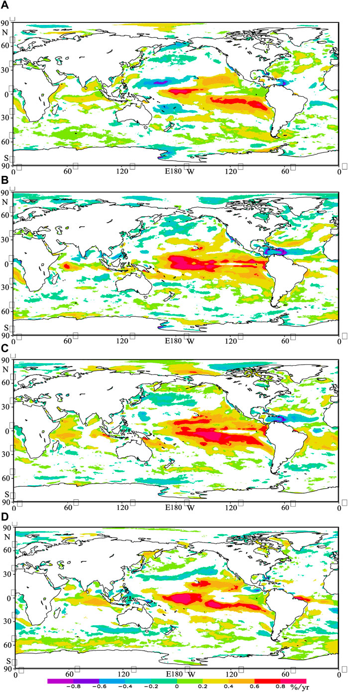
FIGURE 8. Climatic trends of the rich level occurrence in MAM (A), JJA (B), SON (C), and DJF (D) in the global ocean. Only area significant at 95% level is presented.

Monthly Trends of Wind Power Density, Effective Wind Speed Occurrence, and Rich Level Occurrence in Key Regions

Through the previous analysis, it is found that there are significant regional differences in the trend of wind energy resources. Referring to Alves (2006), the global oceans were divided into several regions: tropical Indian Ocean (TIO), extratropical south Indian (ETSI), extratropical North Pacific (ETNP), tropical Pacific Ocean (TPO), extratropical South Pacific (ETSP), extratropical North Atlantic (ETNA), tropical Atlantic Ocean (TAO), and extratropical South Atlantic (ETSA), as shown in Figure 9, to calculate and compare the climatic trends of WPD, EWSO, and RLO of the aforementioned regions in each month, as shown in Table 1.

FIGURE 9

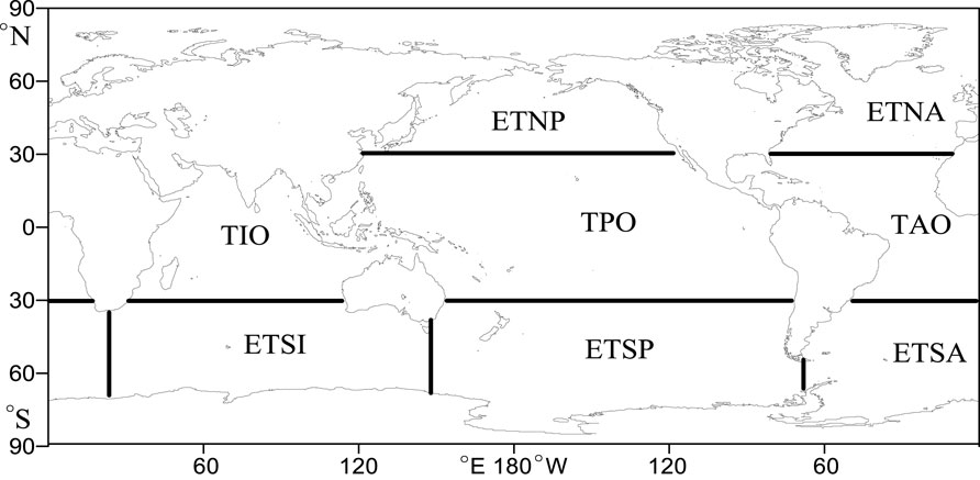
FIGURE 9. Key areas: tropical Indian Ocean (TIO), extratropical south Indian (ETSI), extratropical North Pacific (ETNP), tropical Pacific Ocean (TPO), extratropical South Pacific (ETSP), extratropical north Atlantic (ETNA), tropical Atlantic Ocean (TAO), and extratropical South Atlantic (ETSA).

TABLE 1

TABLE 1. Climatic trends of WPD, EWSO, and RLO in several key regions.

In the TIO, the WPD, EWSO, and RLO have significant annual increasing trends of 0.40 (W/m²)/yr, 0.11%/yr, and 0.08%/yr separately, with WPD passing the 0.01 reliability level and EWSO and RLO passing the 0.001 reliability level. The WPD, EWSO, and RLO tend to increase significantly or to be gentle in each month, which is beneficial for wind energy development. The WPD has significant increasing trends in March, September, and December. The WPD has a significant decreasing trend in August, meaning a decrease in the strength of the southwest monsoon. The trend for the rest of the month is gentle. The EWSO has a significant increasing trend in January, March, May, July, September, October, and December. The increasing trend of RLO is mainly reflected in March, September and October.

In ETSI, the WPD increases significantly year by year of 0.98 (W/m²)/yr. The EWSO and RLO do not exhibit significant annual variation for the past 36 years. The increase of WPD mainly reflects in January, April, and May.

In the ETNP, the WPD, EWSO, and RLO exhibit a slight decreasing trend, but do not pass the significant reliability test.

In the TPO, the WPD, EWSO, and RLO increase year by year significantly of 0.83 (W/m²)/yr, 0.17%/yr, and 0.19%/yr separately, and the trends passed the 0.001 reliability test 1level. The WPD tends to be flat in March, May, and November, and shows significant increases in the rest of the months. The EWSO and RLO trend to be flat in May, and show significant increases in the rest of the months.

In the ETSP, the WPD, EWSO, and RLO have significant annual increasing trends of 1.64 (W/m²)/yr, 0.03%/yr, and 0.06%/yr separately. The annual trends of WPD and EWSO passed the 0.01 reliability test level, and the annual trend of RLO passed the 0.001 reliability test level.

In the ETNA, there is no significant annual trend in WPD. The EWSO and RLO exhibit significant annual increasing trends of 0.04%/yr.

In TAO, the WPD, EWSO, and RLO have significant annual increasing trends of 0.38 (W/m²)/yr, 0.06%/yr, and 0.07%/yr separately.

In the ETSA, the WPD, EWSO, and RLO have significant annual increasing trends of 1.01 (W/m²)/yr, 0.02%/yr, and 0.04%/yr separately.

The annual increasing trend of WPD is strongest in the southern westerlies, especially the ETSP, of about 1.64 (W/m²)/yr. The annual increasing trends of EWSO and RLO are strongest in the tropical waters, especially the TPO, of 0.17%/yr and 0.19%/yr separately.

Abrupt Change of Wind Power Density, Effective Wind Speed Occurrence, and Rich Level Occurrence in Key Regions

From the previous analysis, the low-latitude waters of the middle Pacific Ocean exhibited significant increasing trends in WPD, EWSO, and RLO. Here the abrupt change of wind energy parameters of this region was calculated using the M-K test.

Using the method in Figure 2, the zonal and annual mean values of WPD of the low-latitude waters of the middle Pacific Ocean for 1979–2014 were obtained. Then, the M-K test is employed to exhibit the abrupt change of WPD. Similarly, the abrupt change of EWSO and RLO of the low-latitude waters of the middle Pacific Ocean is exhibited, as shown in Figure 10. About the WPD (Figure 10A), the UF and UB lines intersect in 1999, 2002, and 2003. Also, the intersecting points are located within the two test lines, meaning that the abrupt change of WPD in this region occurred at the end of the 20th century and the beginning of the 21st century. It is also worth noting that the UF line shows a gentle annual variation for the period 1979–1994, while an evident increasing trend for the period 1994–2014. It means that the significant increasing trend of WPD of the low-latitude waters of the middle Pacific Ocean is mainly dominated by the period of 1994–2014. A similar long-term trend and abrupt change can also be found in the EWSO and RLO in the low-latitude waters of the middle Pacific Ocean.

FIGURE 10

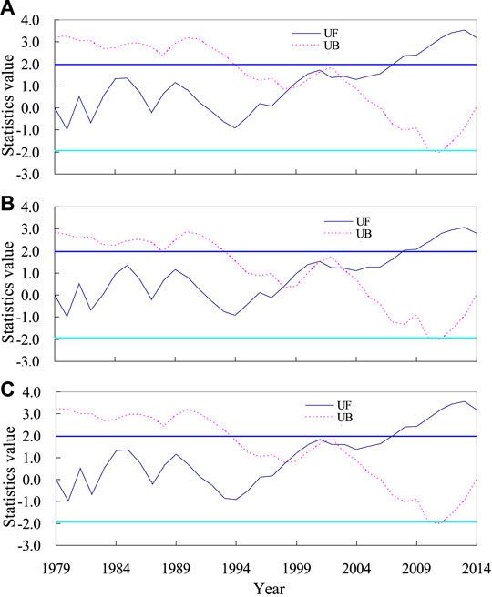
FIGURE 10. M-K test of the WPD (A), EWSO (B), and RLO (C) in the low-latitude waters of the middle Pacific Ocean.

The method in Figure 10 was used to calculate the abrupt change of WPD, EWSO, and RLO in the TIO, ETSI, ETNP, TPO, ETSP, ETNA, TAO, and ETSA, as shown in Figure 11.

FIGURE 11

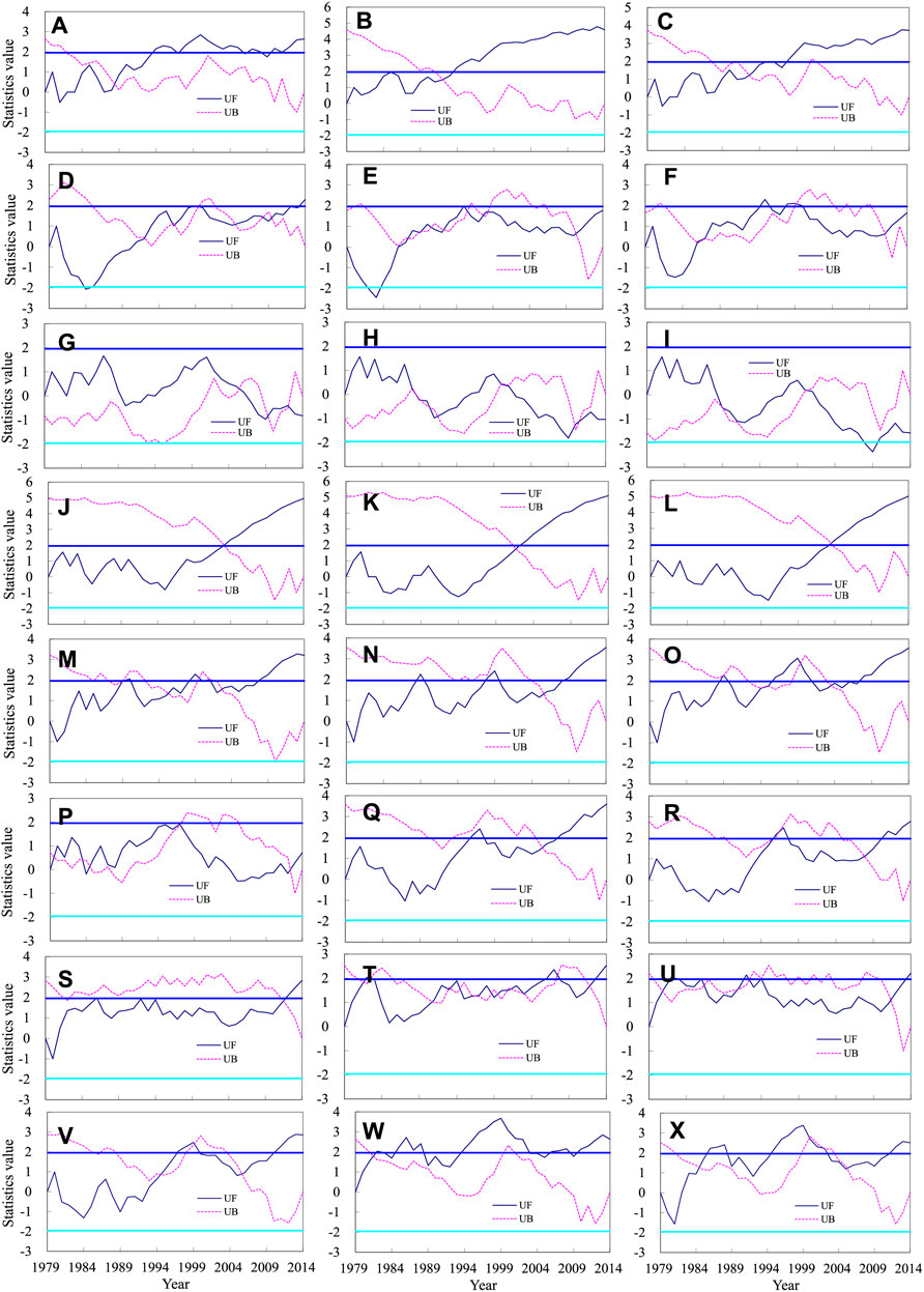
FIGURE 11. M-K test of the WPD (left), EWSO (middle), and RLO (right) in the tropical Indian Ocean (A–C), extratropical south Indian (D–F), extratropical North Pacific (G–I), tropical Pacific Ocean (J–L), extratropical South Pacific (M–O), extratropical North Atlantic (P–R), tropical Atlantic Ocean (S–U), and extratropical South Atlantic (V–X).

In the TIO, the wind energy has an evident abrupt change, with abrupt periods of WPD, EWSO, and RLO occurred in 1988, 1992, and 1993 separately. From the UF line, the WPD exhibited an evident increasing trend for the period 1988–2000 and a gentle annual variation for 2000–2014, meaning that the annual increasing trend of WPD in the TIO is mainly dominated by the period 1988–2000. The annual increasing trends of EWSO and RLO are mainly reflected for the period 1988–2014.

In the ETSI, the abrupt change of wind energy is complex and not evident. The WPD, EWSO, and RLO have an evident increasing trend for the period 1984–1994.

In the ETNP, the abrupt change of wind energy is complex and not evident. The WPD, EWSO, and RLO have an evident decreasing trend in the beginning of the 21st century.

In the TPO, the abrupt change of wind energy occurred in the early 21st century. The annual increasing trends of WPD, EWSO, and RLO are mainly reflected for the period 1995–2014.

In the ETSP, the abrupt change of wind energy is complex and not evident.

In the ETNA, the abrupt change of WPD is not evident. The abrupt change of EWSO and RLO occurred in 2006 and 2008 separately. The WPD slowly increases for 1979–1997 and decreases for the period 1997–2005. The EWSO and RLO have two evident increasing periods: 1991–1997 and 2004–2014.

In the TAO and ETSA, the abrupt change of wind energy is not evident.

As a whole, the climatic trends of wind energy parameters have a good agreement with Figure 5.

Discussions

Thomas et al. (2008) found an increasing WS trend of 4 (cm/s)/yr from 1982 to 2002 over most of the global oceans. Young et al. (2011) presented an increasing WS globally over the period 1991–2008, based on an 18-year database of calibrated and validated satellite altimeter measurements. Capps and Zender (2010) analyzed the global oceanic WS trend for the period 1988–2011, based on the Cross-Calibrated, Multi-Platform (CCMP) wind data. They pointed out that the sea surface WS in most of the global oceans significantly increased for this period with a rate of 1–11 (cm/s)/yr, and the area with a strong increasing trend is mainly located in the mid-low-latitude waters of the Pacific Ocean. There is a good agreement between this study and the previous studies.

Capps and Zender (2010) also stated that the annual mean WS variability was mainly caused by the variability of the occurrences of WS greater than Class 5. In this study, the EWSO exhibits a significant increasing trend. And the spatial distribution of the trend of EWSO has a good agreement with that of WS. Obviously, the result has a good agreement with Zheng et al. (2016). Previous studies by Young et al. (2011), Gulev and Grigotieva (2004); Gulev and Grigorieva (2006), Gulev and Hasse (1999), and Bertin et al. (2013) provided evidence that the long-term increase of WS can be superimposed onto the inter-annual variability controlled by an oscillating phenomenon, such as North Atlantic Oscillation (NAO) over the North Atlantic Ocean, and the El Niño over the Pacific Ocean. Wan (2012) noted that the oscillating phenomenon, such as the ENSO, could contribute to the inter-annual variations of wind power. Zheng et al. (2016) found a close correlation between the nino3 index and the occurrence of WS greater than Class 5 in the tropical waters, especially the tropical waters of the Pacific Ocean. In their result, there is a positive correlation in the low-latitude waters of the middle North Pacific Ocean, meaning that the increase of sea surface temperature (SST) will result in the increase of occurrence of WS greater than Class 5. Zheng et al. (2017) pointed out that there is a noticeable negative correlation between the WPD of lagging 3 months and nino3 index in most of the North Atlantic Ocean. The long-term trend of WPD in the Pacific Ocean may also be attributed to the relationship between the nino3 index and the occurrence of WS greater than Class 5. Reguero et al. (2015) take the lead in analyzing the correlations between the wave energy and key oscillating phenomenon in the global oceans. They found that the influence of the NAO and Atlantic Multidecadal Oscillation (AMO) patterns in the northern and southern hemispheres, respectively.

Correlations Between Wind Energy and Key Oscillating Phenomenon

To reveal the mechanism of the climatic variation of wind energy, research on the relationship between WPD and key important oscillating phenomenon in the global oceans was carried out, as shown in Figure 12.

FIGURE 12

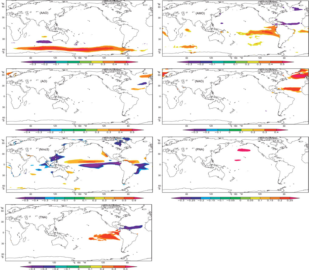
FIGURE 12. Correlations between WPD and AAO, WPD and AMO, WPD and AO, WPD and NAO, WPD and nino3, WPD and PNA, and WPD and TNA.

AAO: the AAO has a widespread and significant influence on the wind energy of the southern hemisphere westerlies (positive correlations) and middle-east of the mid-latitude waters of the South Indian Ocean (negative correlations). The strong AAO indicates the deepening of low pressure around the Antarctic Pole and the strengthening of westerly winds at mid-high latitude. At the same time, the winds in the mid-low latitude weaken.

AMO: the AMO has a significant impact on the mid-east area of the tropical waters of the South Pacific Ocean (positive correlation), tropical waters of the North Atlantic Ocean (negative correlation), and south water of Greenland (negative correlation).

AO: the AO has a significant impact on the North Atlantic Ocean. In the North Atlantic Ocean, the correlations exhibit a spatial distribution of positive–negative–positive from the mid-high latitude to the low latitude. The AO is the change of atmospheric pressure between the mid-latitude region and the arctic region in the northern hemisphere. When the arctic oscillation is in the positive phase, the pressure difference of these systems is stronger than normal, which limits the cold air in the polar region to spread southward. In this case, the winds will strengthen in the high latitude and will weaken in the middle latitude.

NAO: the NAO has a significant impact on the mid-high latitude waters (A large sea area surrounds Greenland, positive correlation) and tropical waters of the North Atlantic Ocean (positive correlation). The NAO is the inverse relationship between the Azores high pressure and the Icelandic low pressure. The strong NAO indicates a large pressure difference between the Azores high pressure and the Icelandic low pressure and a strong westerly wind in the middle latitude of the North Atlantic Ocean.

Nino3: the nino3 index has a positive influence on the tropical water of the North Pacific Ocean, tropical water of the North Atlantic Ocean. It has a negative influence on the tropical water of the South Pacific Ocean, tropical water of the South Atlantic Ocean and the northern region of the South China Sea, and a large region around the Taiwan Island.

PNA: the Pacific/North American Pattern (PNA) has a significant impact on a small region of the middle of the mid-latitude of the North Pacific Ocean.

TNA: the Tropical Northern Atlantic Index (TNA) has a negative impact on the tropical waters of the North Atlantic Ocean, and has a positive impact on the east region of tropical waters of the South Pacific Ocean.

Periods of Wind Power Density, Effective Wind Speed Occurrence, and Rich Level Occurrence in Key Regions

In this section, the wavelet analysis method is employed to analyze the variation period of WPD in the key regions. Using the method in Figure 2, the zonal and annual average values of WPD in the TIO for 1979–2014 were obtained. Then, the variation periods were analyzed using wavelet analysis. Similarly, the variation periods of WPD in the ETSI, ETNP, TPO, ETSP, ETNA, TAO, and ETSA were calculated, as shown in Figure 13. The WPD in the TIO, ETNP, and ETNA has a definite period of 3–6 years. Also, this phenomenon can also be found in other regions, but not so evident.

FIGURE 13

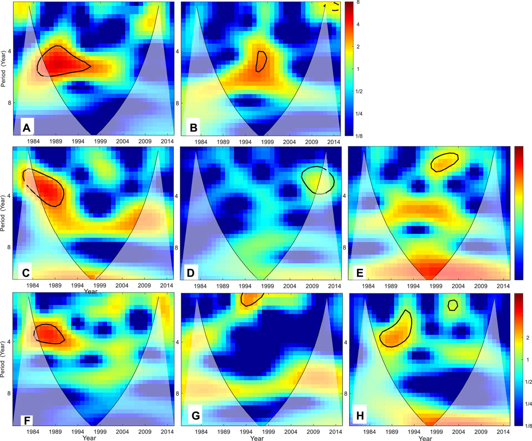
FIGURE 13. Wavelet analysis of the WPD in the tropical Indian Ocean (A), extratropical south Indian (B), extratropical North Pacific (C), tropical Pacific Ocean (D), extratropical South Pacific (E), extratropical North Atlantic (F), tropical Atlantic Ocean (G), and extratropical South Atlantic (H).

This study also pays attention to the variation period of WPD, EWSO, and RLO in the Arabian Sea, the Bay of Bengal, and the South China Sea, as shown in Figure 14. Obviously, the WPD, EWSO, and RLO in the Arabian Sea and the Bay of Bengal, and the WPD in the South China Sea have a significant common period of approximately 5 years. The EWSO and RLO in the South China Sea also have a period of approximately 5 years, but not as evident as the WPD.

FIGURE 14

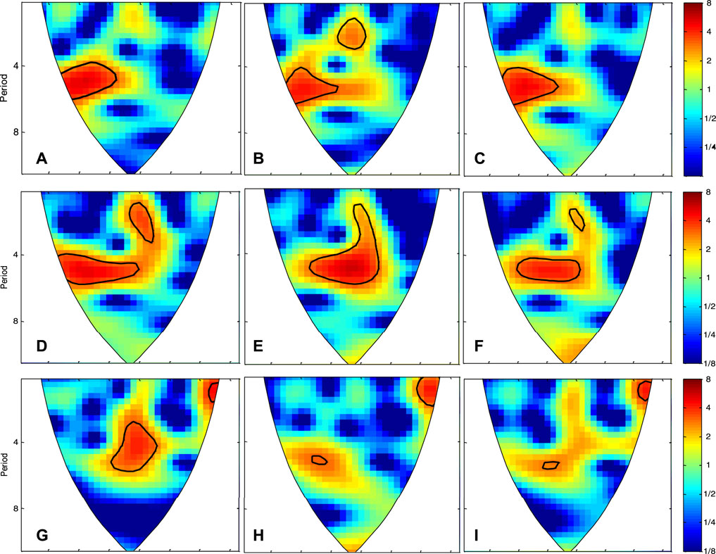
FIGURE 14. Wavelet analysis of the WPD (left), EWSO (middle), and RLO (right) in the Arabian Sea (A–C), the Bay of Bengal (D–F), and the South China Sea (G–I) for the period 1979–2014.

Just as the previous discussion, the wind energy has a close relationship with some important oscillating phenomena, such as AAO, AO, and AMO. To detect the correlation between the wind energy and important oscillating phenomenon, the variation period of the nino3 index for the period 1979–2014 is also calculated, as shown in Figure 15. Obviously, the nino3 index exhibits a significant period of approximately 5 years. Former research studies also pointed out that there exists a close correlation between the sea surface WS and the El Niño phenomenon in the Pacific Ocean and North Atlantic Ocean (Liu et al., 2008; Zheng and Pan, 2014; Guo et al., 2018; Wang, 2020). Through this study, a common period of approximately 5 years among the wind energy parameters and nino3 index was found, which has a good agreement with the previous research.

FIGURE 15

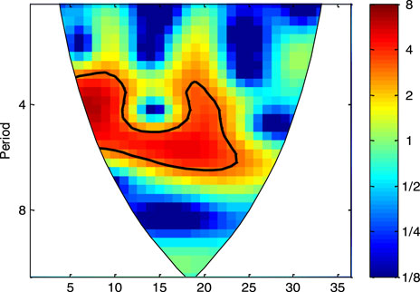
FIGURE 15. Wavelet analysis of the nino3 index for the period 1979–2014.

Conclusion and Prospect

Based on the ERA-Interim wind product for 1979–2014, this study presented the climatic trends of series of key parameters (WPD, EWSO, and RLO) of wind energy resources in the global oceans, including the overall annual trends, the regional difference and seasonal difference of the trend, abrupt changes, and variation of wind energy in the key region. The correlations between the wind energy and key oscillating phenomenon were also calculated. The main conclusions are as follows:

The global oceans are rich in wind energy resources. The multi-year average WPD in most of the global ocean is greater than 200 W/m², while only some small regions in the low-latitude waters are below 200 W/m². The EWSO is >60% in most of the global oceans, meaning an optimistic wind energy available rate globally. There also exist several large areas of EWSO in the mid-low-latitude waters of global oceans (even >90% in the large center), meaning an optimistic wind energy utilization rate, although they are not distributed in the large area of WPD. The spatial distribution of the RLO is similar to that of EWSO.

For the past 36 years, the global ocean exhibits overall increasing trends in WPD [0.698 (W/m²)/yr], EWSO (0.076%/yr), and RLO (0.090%/yr). The increasing trends of WPD, EWSO, and RLO in the southern hemisphere oceans are much stronger than that in the northern hemisphere oceans.

The annual trend of wind energy exhibits an evident regional difference. The annual increasing trend of WPD is strongest in the southern westerlies, especially the ETSP, of about 1.64 (W/m²)/yr. The areas with significant increasing trends in WPD are mainly distributed in the Somali waters of 1–3 (W/m²)/yr, equator waters of the south Indian Ocean of 0–2 (W/m²)/yr, the mid-low latitude of the middle and east of the Pacific Ocean of 0–4 (W/m²)/yr, the low latitude of the South Atlantic Ocean of 0–2 (W/m²)/yr, and part of the southern hemisphere westerlies of 3–6 (W/m²)/yr. The area range with a significant decreasing trend is small and mainly located in the south and southeast coasts of Greenland and middle of the North Pacific Ocean westerly. The annual increasing trends of EWSO and RLO are strongest in the tropical waters, especially the TPO, of 0.17%/yr and 0.19%/yr, separately.

About the seasonal difference of the trends, the WPD in most of the global oceans has a significant increasing trend or no significant variation in each season, while only some small regions have a significant increasing trend. Regardless of the season, areas with significant increasing trends are mainly distributed in the mid-low-latitude waters of global oceans and part of the southern hemisphere westerlies. The increasing trend of WPD in different regions is dominated by different seasons. The increasing trend of WPD in the mid-low-latitude waters of global oceans can be reflected in each season. The increasing trend in the southern hemisphere westerlies can be seen in MAM and DJF. The decreasing trend in the low-latitude waters of the North Atlantic Ocean is dominated by JJA and SON. The characteristic seasonal difference of the long-term trends of EWSO and RLO is similar to that of the WPD.

The climatic trends of wind energy are dominated by different time periods. The annual increasing trend of WPD in the TIO is mainly dominated by the period 1988–2000. The annual increasing trends of EWSO and RLO in the TIO are mainly reflected for 1988–2014. The annual increasing trends of WPD, EWSO, and RLO in the TPO are mainly reflected for the period 1995–2014.

There is no evident abrupt change of wind energy in the extratropical waters (ETSI, ETNP, ETSP, ETNA, ETSA) and TAO. The abrupt periods of wind energy in the TIO and TPO occurred at the end of the 20th century and in the beginning of the 21st century. The WPD, EWSO, and RLO of the South China Sea, the Arabian Sea, and the Bay of Bengal and nino3 index share a common period of approximately 5 years.

There is a close relationship between the wind energy and key oscillating phenomenon in the global oceans. The AAO has a positive influence on the wind energy of the southern hemisphere westerlies. The AMO has a positive impact on the mid-east area of the tropical waters of the South Pacific Ocean. The AO has a positive–negative–positive impact on the wind energy of the North Atlantic Ocean from the mid-high latitude to the low latitude. The NAO has a positive impact on the mid-high latitude waters and tropical waters of the North Atlantic Ocean. The nino3 index has a significant influence on the tropical waters of the Pacific Ocean and tropical waters of the Atlantic Ocean. The TNA has a negative impact on the tropical waters of the North Atlantic Ocean and a positive impact on the east region of tropical waters of the South Pacific Ocean.

In this study, the data used in this study are the ERA-Interim reanalysis. In 2019, a newer version of ECMWF reanalysis—ERA-5—is available. In the future work, it is necessary to employ the ERA5 data to analyze the trend of global oceanic wind energy and compare the wind energy trend using ERA-Interim data and the wind energy trend using ERA5 data. This study exhibits the wind energy trends of 10 m above the sea surface. Liu et al. (2018) analyzed the wind resource potential at different heights using a long-term tower measurement. Similarly, it is necessary to analyze the long-term trends of wind energy at different heights above the sea surface. Also, the energy returns on energy and carbon investment of wind energy farms (Xydis, 2015), factors influencing citizens’ acceptance and non-acceptance of wind energy, etc. should also be focused in the future work. In addition, countries and regions can carry out related policy and long-term plans according to the climatic variation of wind energy resources.

Data Availability Statement

Publicly available datasets were analyzed in this study. These data can be found here: ERA-Interim wind data (available at https://apps.ecmwf.int/datasets/data/Interim-full-daily/levtype = sfc/).

Author Contributions

C-WZ, W-KZ, X-LW, CS, WZ, and Z-NX: conceptualization and methodology. C-TY and YW: methodology and data curation. S-DJ and DW: investigation and methodology. XJ and Y-GC: original draft preparation. X-FZ and D-JW: software and validation. D-CY, YW, WL and Y-YT: revise the manuscript.

Funding

This work was supported by the open fund project of the Shandong Provincial Key Laboratory of Ocean Engineering, Ocean University of China (No. kloe201901), and the Open Research Fund of State Key Laboratory of Estuarine and Coastal Research (Grant number SKLEC-KF201707).

Conflict of Interest

The authors declare that the research was conducted in the absence of any commercial or financial relationships that could be construed as a potential conflict of interest.

Publisher’s Note

All claims expressed in this article are solely those of the authors and do not necessarily represent those of their affiliated organizations, or those of the publisher, the editors, and the reviewers. Any product that may be evaluated in this article, or claim that may be made by its manufacturer, is not guaranteed or endorsed by the publisher.

Acknowledgments

The authors would also like to thank the ECMWF for providing the ERA-Interim wind data (available at https://apps.ecmwf.int/datasets/data/interim-full-daily/levtype=sfc/).

References

Akpınar, A., Jafali, H., and Rusu, E. (2019). Temporal Variation of the Wave Energy Flux in Hotspot Areas of the Black Sea. Sustainability 11 (3), 562. doi:10.3390/su11030562

CrossRef Full Text | Google Scholar

Akpınar, A., Kutupoğlu, V., Bingölbali, B., and Çalışır, E. (2021). Spatial Characteristics of Wind and Wave Parameters over the Sea of Marmara. Ocean Eng. 222, 108640. doi:10.1016/j.oceaneng.2021.108640

CrossRef Full Text | Google Scholar

Alves, J.-H. G. M. (2006). Numerical Modeling of Ocean Swell Contributions to the Global Wind-Wave Climate. Ocean Model. 11, 98–122. doi:10.1016/j.ocemod.2004.11.007

CrossRef Full Text | Google Scholar

Amirinia, G., Kamranzad, B., and Mafi, S. (2017). Wind and Wave Energy Potential in Southern Caspian Sea Using Uncertainty Analysis. Energy 120, 332–345. doi:10.1016/j.energy.2016.11.088

CrossRef Full Text | Google Scholar

Bertin, X., Prouteau, E., and Letetrel, C. (2013). A Significant Increase in Wave Height in the North Atlantic Ocean over the 20th century. Glob. Planet. Change 106, 77–83. doi:10.1016/j.gloplacha.2013.03.009

CrossRef Full Text | Google Scholar

Bosch, J., Staffell, I., and Hawkes, A. D. (2018). Temporally Explicit and Spatially Resolved Global Offshore Wind Energy Potentials. Energy 163, 766–781. doi:10.1016/j.energy.2018.08.153

CrossRef Full Text | Google Scholar

Capps, S. B., and Zender, C. S. (2010). Estimated Global Ocean Wind Power Potential from QuikSCAT Observations, Accounting for Turbine Characteristics and Siting. J. Geophys. Res. 115, 12679–12691. doi:10.1029/2009jd012679

CrossRef Full Text | Google Scholar

Capps, S. B., and Zender, C. S. (2009). Global Ocean Wind Power Sensitivity to Surface Layer Stability. Geophys. Res. Lett. doi:10.1029/2008GL037063L09801

CrossRef Full Text | Google Scholar

Chen, X., Foley, A., Zhang, Z., Wang, K., and O'Driscoll, K. (2020). An Assessment of Wind Energy Potential in the Beibu Gulf Considering the Energy Demands of the Beibu Gulf Economic Rim. Renew. Sust. Energ. Rev. 119, 109605. doi:10.1016/j.rser.2019.109605

CrossRef Full Text | Google Scholar

Dee, D. P., Uppala, S. M., Simmons, A. J., Berrisford, P., Poli, P., Kobayashi, S., et al. (2011). The ERA-Interim Reanalysis: Configuration and Performance of the Data Assimilation System. Q.J.R. Meteorol. Soc. 137, 553–597. doi:10.1002/qj.828

CrossRef Full Text | Google Scholar

Devlin, J., Li, K., Higgins, P., and Foley, A. (2017). Gas Generation and Wind Power: A Review of Unlikely Allies in the United Kingdom and Ireland. Renew. Sust. Energ. Rev. 70, 757–768. doi:10.1016/j.rser.2016.11.256

CrossRef Full Text | Google Scholar

Earl, N., Dorling, S., Hewston, R., and Glasow, R. V. (1980-20102013). Variability in U.K. Surface Wind Climate. J. Clim. 26 (4), 1172–1191.

Google Scholar

Esteban, M. D., Diez, J. J., López, J. S., and Negro, V. (2009). Integral Management Applied to Offshore Wind Farms. J. Coastal Res. 56, 1204–1208.

Google Scholar

European Centre for Medium-Range Weather Forecasts (ECMWF) ERA-interim Wind Data [EB/OL]. (2011-01-01) [ 2015-06-22]. https://apps.ecmwf.int/datasets/data/interim-full-daily/levtype=sfc/.

Google Scholar

Gulev, S. K., and Grigorieva, V. (2006). Variability of the winter Wind Waves and Swell in the North Atlantic and North Pacific as Revealed by the Voluntary Observing Ship Data. J. Clim. 19, 5667–5685. doi:10.1175/jcli3936.1

CrossRef Full Text | Google Scholar

Gulev, S. K., and Grigotieva, V. (2004). Last century Changes in Ocean Wind Wave Height from Global Visual Wave Data. Geophys. Res. Lett. 31, L24302. doi:10.1029/2004GL021040

CrossRef Full Text | Google Scholar

Gulev, S. K., and Hasse, L. (1999). Changes of Wind Waves in the north Atlantic over the Last 30 Years. Int. J. Climatol. 19, 1091–1117. doi:10.1002/(sici)1097-0088(199908)19:10<1091::aid-joc403>3.0.co;2-u

CrossRef Full Text | Google Scholar

Guo, Q., Xu, X., Zhang, K., Li, Z., Huang, W., Mansaray, L., et al. (2018). Assessing Global Ocean Wind Energy Resources Using Multiple Satellite Data. remote sensing 10, 100. doi:10.3390/rs10010100

CrossRef Full Text | Google Scholar

Higgins, P., Foley, A. M., Douglas, R., and Li, K. (2014). Impact of Offshore Wind Power Forecast Error in a Carbon Constraint Electricity Market. Energy 76, 187–197. doi:10.1016/j.energy.2014.06.037

CrossRef Full Text | Google Scholar

Higgins, P., and Foley, A. (2014). The Evolution of Offshore Wind Power in the United Kingdom. Renew. Sust. Energ. Rev. 37, 599–612. doi:10.1016/j.rser.2014.05.058

CrossRef Full Text | Google Scholar

Jiang, B., Wei, Y., Ding, J., Zhang, R., Liu, Y., Wang, X., et al. (2019). Trends of Sea Surface Wind Energy over the South China Sea. J. Ocean. Limnol. 37 (5), 1510–1522. doi:10.1007/s00343-019-8307-6

CrossRef Full Text | Google Scholar

Khojasteh, D., Mousavi, S. M., Glamore, W., and Iglesias, G. (2018). Wave Energy Status in Asia. Ocean Eng. 169, 344–358. doi:10.1016/j.oceaneng.2018.09.034

CrossRef Full Text | Google Scholar

Liu, J., Gao, C. Y., Ren, J., Gao, Z., Liang, H., and Wang, L. (2018). Wind Resource Potential Assessment Using a Long Term tower Measurement Approach: A Case Study of Beijing in China. J. Clean. Prod. 174, 917–926. doi:10.1016/j.jclepro.2017.10.347

CrossRef Full Text | Google Scholar

Liu, W. T., Tang, W., and Xie, X. (2008). Wind Power Distribution over the Ocean. Geophys. Res. Lett. 35, L13808. doi:10.1029/2008GL034172

CrossRef Full Text | Google Scholar

Liu, Y., Yin, X., and Xu, Y. (2017). The Analysis of Gales over the “Maritime Silk Road” with Remote Sensing Data. Acta Oceanol. Sin. 36 (9), 15–22. doi:10.1007/s13131-017-1106-z

CrossRef Full Text | Google Scholar

Miao, W., Jia, H., Wang, D., Parkinson, S., Crawford, C., and Djilali, N. (2012). Active Power Regulation of Wind Power Systems through Demand Response. Sci. China Technol. Sci. 55, 1667–1676. doi:10.1007/s11431-012-4844-3

CrossRef Full Text | Google Scholar

Reguero, B. G., Losada, I. J., and Méndez, F. J. (2015). A Global Wave Power Resource and its Seasonal, Interannual and Long-Term Variability. Appl. Energ. 148, 366–380. doi:10.1016/j.apenergy.2015.03.114

CrossRef Full Text | Google Scholar

Soares, P. M. M., Lima, D. C. A., and Nogueira, M. (2020). Global Offshore Wind Energy Resources Using the new ERA-5 Reanalysis. Environ. Res. Lett. 15, 1040a2. doi:10.1088/1748-9326/abb10d

CrossRef Full Text | Google Scholar

Song, L., Liu, Z., and Wang, F. (2015). Comparison of Wind Data from ERA-Interim and Buoys in the Yellow and East China Seas. Chin. J. Ocean. Limnol. 33 (1), 282–288. doi:10.1007/s00343-015-3326-4

CrossRef Full Text | Google Scholar

Thomas, B. R., Kent, E. C., Swail, V. R., and Berry, D. I. (2008). Trends in Ship Wind Speeds Adjusted for Observation Method and Height. Int. J. Climatol. 28 (6), 747–763. doi:10.1002/joc.1570

CrossRef Full Text | Google Scholar

Wan, Y. H. (2012). Long-term Wind Power Variability. Colorado: National Renewable Energy Laboratory.

Google Scholar

Wang, J. (2020). Determining the Most Accurate Program for the Mann-Kendall Method in Detecting Climate Mutation. Theor. Appl. Climatol 142, 847–854. doi:10.1007/s00704-020-03333-x

CrossRef Full Text | Google Scholar

Wen, Y., Kamranzad, B., and Lin, P. (2021). Assessment of Long-Term Offshore Wind Energy Potential in the South and Southeast Coasts of China Based on a 55-year Dataset. Energy 224, 120225. doi:10.1016/j.energy.2021.120225

CrossRef Full Text | Google Scholar

Xydis, G. (2015). A Wind Energy Integration Analysis Using Wind Resource Assessment as a Decision Tool for Promoting Sustainable Energy Utilization in Agriculture. J. Clean. Prod. 96, 476–485. doi:10.1016/j.jclepro.2013.11.030

CrossRef Full Text | Google Scholar

Xydis, G. (2016). A Wind Resource Assessment Around Large Mountain Masses: The Speed-Up Effect. Int. J. Green Energ. 13 (6), 616–623. doi:10.1080/15435075.2014.993763

CrossRef Full Text | Google Scholar

Young, I. R., Zieger, S., and Babanin, A. V. (2011). Global Trends in Wind Speed and Wave Height. Science 332 (6028), 451–455. doi:10.1126/science.1197219

PubMed Abstract | CrossRef Full Text | Google Scholar

Zheng, C.-w., Pan, J., and Li, J.-x. (2013). Assessing the China Sea Wind Energy and Wave Energy Resources from 1988 to 2009. Ocean Eng. 65, 39–48. doi:10.1016/j.oceaneng.2013.03.006

CrossRef Full Text | Google Scholar

Zheng, C. W., Li, C. Y., and Li, X. Recent Decadal Trend in the North Atlantic Wind Energy Resources. Adv. Meteorology, 2017, Volume 2017, Article ID 7257492, 1, 8 pages. doi:10.1155/2017/7257492

CrossRef Full Text | Google Scholar

Zheng, C. w., and Pan, J. (2014). Assessment of the Global Ocean Wind Energy Resource. Renew. Sust. Energ. Rev. 33, 382–391. doi:10.1016/j.rser.2014.01.065

CrossRef Full Text | Google Scholar

Zheng, C. W., Pan, J., and Li, C. Y. (2016). Global Oceanic Wind Speed Trends. Ocean Coastal Manag. 129, 15–24. doi:10.1016/j.ocecoaman.2016.05.001

CrossRef Full Text | Google Scholar