Prediction of Remaining Useful Life of the Lithium-Ion Battery Based on Improved Particle Filtering

Remaining useful life (RUL) prediction of lithium-ion batteries plays an important role in battery failure prediction and health management (PHM). By accurately predicting the RUL of the battery, the battery can be replaced accordingly, thereby effectively avoiding the occurrence of an accident and ensuring the normal operation of the entire system. In the prediction of the remaining service life of lithium-ion batteries, it is difficult to ensure accuracy due to the problem of particle degradation and the influence of singular values in the particle filter algorithm. In view of these problems, this article introduces the unscented Kalman algorithm to improve the particle filter algorithm from the perspective of re-weighting the particles, so as to improve the accuracy of the prediction results of the remaining service life of lithium-ion batteries. The improved particle filter is simulated and verified using the battery sample data in the Arbin experimental test platform. Comparing the simulation results with the traditional particle filter method, when the number of reference samples is the same, the PDF width of the prediction results of the improved particle filter algorithm is slightly smaller than that of the particle filter algorithm, indicating that the fluctuation of the prediction result is more accurate. It is proved that the improved particle filter method proposed in this article can provide more accurate battery RUL prediction results and can effectively improve the accuracy and robustness of the remaining service life prediction of lithium-ion batteries.

1 Introduction

In modern production and life, the electronic system has become indispensable, and people have been paying more and more attention to the reliability and safety of its operation. Electronic system fault prediction and health management (Zheng et al., 2018; Saxena et al., 2019) has become one of the hotspots in recent years, and fault prediction is, especially important in PHM technology. This means predictive diagnostics for systems based on their current or historical state to determine their remaining useful life (Wang and Mamo, 2018; Wang et al., 2020a). On this basis, analyzing and managing the system status can effectively reduce or avoid catastrophic losses caused by system failures.

As the energy source for many key electronic devices and systems (McTurk et al., 2020), lithium-ion batteries play a crucial role in the whole electronic system; are now widely used in portable electronic devices, such as laptops, video cameras, and mobile communication tools; and have been successfully promoted in important fields such as new energy vehicles and aerospace (Chen et al., 2019; Liu et al., 2019a). However, with the wide application of lithium-ion batteries, their own health management, performance degradation, safety maintenance, and remaining life estimation have also become urgent problems to be solved. Condition monitoring, performance analysis, and application management of Li-ion batteries have become one of the challenges in the field of electronic system failure prediction and health management (Hu and Tang, 2018).

Since the battery itself is a complex electrochemical system, the lithium battery system is highly nonlinear, with multi-spatial scales (such as nano-active materials, mm cells, and battery packs) and multi-time scale aging, which is difficult to accurately model (Huangfu et al., 2018; Wang et al., 2020b). In order to effectively evaluate the reliability of lithium-ion batteries, it is particularly important to predict the remaining useful life of lithium-ion batteries. The remaining service life of a Li-ion battery is defined as the number of remaining charge–discharge cycles before the battery capacity drops to the rated failure threshold (Zhao et al., 2019). Scholars have conducted a lot of research on RUL prediction of Li-ion batteries, and great progress has been made in battery modeling and state estimation methods, which can be broadly classified into three categories: mechanistic model-based methods, data-driven methods, and model- and data-driven fusion-based methods (Liu et al., 2019b; Feng et al., 2020; Nagulapati et al., 2021).

The model-based methods rely less on historical data and can carry out forecasting research even without too many sample data. This approach focuses on identifying the correspondence between observables and health indicators by establishing a physical model of the degradation process that affects battery life (Wang et al., 2020c). Chao et al. (2016) combined the electrochemical model of the battery and proposed a new particle filter framework for the RUL prediction of lead-acid batteries, which regarded the model parameters reflecting battery degradation as state variables. Li et al. (2016) developed a simplified multi-particle model through a prediction-correction strategy and quasi-linearization, which allowed researchers to accelerate the process of battery design, aging analysis, and RUL estimation. Si et al. (2015) proposed an adaptive nonlinear prediction model that uses the system’s observation data history so far to estimate the battery RUL. Because this method needs to build a system mechanism model based on the physics, chemistry, or experience of the predicted battery itself, it is difficult to obtain an accurate model under the influence of different external conditions (Qian and Yan, 2015).

The data-driven method does not need to consider the material properties, structure, and complicated electrochemical reaction process of the battery itself. It only needs to extract the historical data of the lithium-ion battery itself and track and learn the trend in the data to achieve the purpose of predicting the RUL of the lithium-ion battery (Ren et al., 2018; Li et al., 2019). Wu et al. (2016) proposed to use a neural network to simulate the relationship between battery constant current charging curve and battery RUL. Patil et al. (2015) proposed a multi-node support vector machine method to predict the remaining useful life of the battery under different working conditions. Zhao et al. (2017) developed a fault diagnosis method for electric vehicle battery systems based on big data statistical methods. Since intelligent algorithms such as vector machines and neural networks used in data-driven methods require a large amount of calculation, how to reduce computational complexity and improve computational efficiency is an urgent difficulty to be solved.

The method based on fusion technology aims to combine the aforementioned model-based and data-driven methods as much as possible, trying to overcome the limitations of the two types of methods, so as to improve the accuracy of prediction by making better use of all available information (Chang et al., 2017; Duan et al., 2020). This method is currently a research hotspot in the prediction of RUL of lithium-ion batteries. Sbarufatti et al. (2017) proposed a lithium-ion battery discharge end-point prediction method based on the combination of particle filter and radial basis function neural network. Wang et al. (2016) constructed a state-space model of lithium-ion battery capacity to evaluate capacity degradation and used a spherical volume particle filter to solve the state-space model. Liu et al. (2017) proposed an improved particle learning framework combined with a battery prediction model to predict the RUL of lithium-ion batteries.

2 Particle Filter and Unscented Kalman Filtering Algorithm

2.1 Particle Filter

The particle filter algorithm is a recursive Bayesian estimation method based on the sequential Monte Carlo idea, which is often used to solve system state estimation problems under non-Gaussian, nonlinear conditions and widely used in static environments or dynamic predictable scenarios.

Since the idea of the particle filtering algorithm is to approximate the posterior probability distribution $P\left(x_k\text{|}{y}_k\right)$ by a set of random particles, the posterior distribution is recursively estimated in real time by using the Monte Carlo sampling method and exploiting the prior distribution of the system and Bayesian estimation. Therefore, we usually assume that the posterior probability density $P\left(x_{k-1}\text{|}{y}_{k-1}\right)$ of the system at the moment k-1 is known, and we use particle filtering to predict the posterior probability density $P\left(x_k\text{|}{y}_k\right)$ of the system at the moment k. Assuming that the prior distribution of the system $P\left(x_k\right)$ is known, then a random sampling sample can be selected based on $P\left(x_k\right)$. After obtaining the marginal distribution of the system $P\left(y_k\right)$ at moment k, the distribution represented by the sampled samples is modified so that the modified sample distribution can approximate the posterior distribution of the system at moment k. When we get more samples, the predicted posterior distribution is closer to the true posterior distribution.

The spatial state model of the system is as follows:

$\{\begin{array}{c}{x}_k=f_k\left(x_{k-1},v_{k-1}\right),\\ y_k=h_k\left(x_k,n_k\right). \end{array}(1)$

In Equation 1, $f_k(\cdot )$ and $h_k(\cdot )$ are the state transition function and measurement function of the system, respectively. Among them, $x_k$ and $y_k$ are the system state and measurement data of the system at moment k, respectively, and $v_k$ and $n_k$ are the process noise and observation noise of the system independently and identically distributed.

The specific implementation steps of the basic particle filter algorithm are as follows:

1) Algorithm data parameter setting:

Number of particles N, process noise $v_k$, observation noise $n_k$, initial state value, and driving matrix $Ф$, etc.

2) Initial setting of particle set:

When k = 0, the set of sampled particles $x_0^i$ is obtained according to the known state prior probability density $P\left(x_0\right)$ of the dynamic system, and the weight of each particle is ${\text{ω}}_0^i$, $i=\mathrm{1,2}\dots N$.

3) Importance distribution:

Assuming that the posterior distribution $P\left(x_{0:k}\text{|}{y}_{1:k}\right)$ is known, the sampled particles obtained from the posterior distribution are the most reliable. However, this posterior distribution is multivariate and nonstandard, and it is very difficult to sample particles directly from this distribution. Therefore, we usually choose to sample from the prior distribution or introduce a similar distribution whose probability density function is known and easy to sample, and this distribution is called the importance distribution.

4) Importance weight calculation:

Before carrying out the system state update of particle filtering and optimization of observations, we need to calculate the weights of particles by the observations at the current moment, and the formula for calculating the weights of particles is as follows:

${\omega }_k\left(x_{0:k}\right)=\frac{p\left(y_{1:\mathrm{k}}|x_{0:k}\right)p\left(x_{0:k}\right)}{q\left(x_{0:k}|y_{1:k}\right)}.(2)$

Since the aforementioned equation is not a recursive formula and ${\omega }_k\left(x_{0:k}\right)$ in the equation is a non-normalized importance weight, in practical applications, the weights of the particles need to be recalculated as the observations are updated, which causes an increase in computational effort. Assuming that the current moment state only considers filtering and does not depend on future observations, the importance function can be rewritten as follows:

$q\left(x_{0:k}\text{|}{y}_{1:k}\right)=q\left(x_0\right){\displaystyle \prod _{j=1}^{k}q\left(x_j\text{|}{x}_{0:j-1},y_{1:j}\right)}.(3)$

Assuming that the system state is consistent with a Markov process at this point, we can obtain:

$p\left(x_{0:k}\right)=p\left(x_0\right){\displaystyle \prod _{j=1}^{k}p\left(x_j\text{|}{x}_{j-1}\right)},(4)$

$p\left(y_{1:k}\text{|}{x}_{0:k}\right)={\displaystyle \prod _{j=1}^{k}p\left(y_j\text{|}{x}_j\right)}.(5)$

Substituting Eqs 3–5 into Equation 2, the following recursive weight formula can be obtained:

${\omega }_k={\omega }_{k-1}\frac{p\left(x_k\text{|}{x}_{k-1}\right)p\left(y_k\text{|}{x}_k\right)}{q\left(x_k\text{|}{x}_{0:k-1},y_{1:k}\right)}.(6)$

Assuming that the prior distribution $p\left(x_k\text{|}{x}_{k-1}\right)$ is taken as the importance distribution, the following equation can be obtained:

$q\left(x_k\text{|}{x}_{0:k-1},y_{1:k}\right)=p\left(x_k\text{|}{x}_{k-1}\right).(7)$

Substituting Equation 7 into Equation 6, we can get:

${\omega }_k={\omega }_{k-1}p\left(y_k\text{|}{x}_k\right).(8)$

Finally, the importance weight is normalized:

${\omega }_k^i=\frac{{\omega }_k^i}{{{\displaystyle \sum }}_{i=1}^N{\omega }_k^i}.(9)$

5) Resampling:

The purpose of resampling is to solve the problem of particle degradation. If $N_{off}=\frac{1}{{{\displaystyle \sum }}_{i=1}^N{\left(W_k^i\right)}^2}$ < $N_{threshold}$, resampling is performed to get a new sample of weights ${\left\{{\tilde{x}}_{0:k,}^i{w}_k^i\right\}}_{i=1}^N$ and reset the weights of all particles such that $w_k^i$ = 1/N, where $N_{threshold}$ is the resampling threshold, which is generally taken as $N_{threshold}$ = 2N/3.

6) Output state estimation:

Mathematical expectations of output sampled particles:

${\tilde{x}}_k^i={\displaystyle \sum _{i=1}^N{w}_k^i{x}_k^i}.(10)$

7) Loop iteration:

Judge whether k is greater than the number of known measured values, if yes, end and exit the algorithm, otherwise return to step 3, and repeat steps 3–6 until the last measurement.

2.2 Unscented Kalman Filtering Algorithm

Instead of approximating the Taylor series expansion term of the nonlinear function, the UKF algorithm approximates the probability density distribution of the state vector in the nonlinear function and then uses the prior mean and covariance to generate a series of determined sigma sampling points, and when these sampling points are passed through the nonlinear system, the posterior mean and covariance of the resulting state vector can be accurate to the third order (Taylor series expansion term) (Zhang et al., 2020). Moreover, UKF does not require the system to be differentiable, so there is no need to derive and calculate complex Jacobian matrices, so the UKF algorithm based on unscented transformation is easier to implement than the extended Kalman filter algorithm, and has higher value in practical applications. At the same time, unlike the local linearization in the extended Kalman filter algorithm, the UKF algorithm does not ignore the higher-order terms and uses the information that the nonlinear system has more state points in the state space, which effectively overcomes the disadvantages of the extended Kalman filter algorithm such as low estimation accuracy and poor stability, and has higher computational accuracy.

First, the basic principle of unscented transformation is introduced. Suppose an n-dimensional random variable x is nonlinearly transformed to obtain y = f(x), and the mean and variance of the random variable x are known to be $\overline{\mathit{X}}$ and $P_x$, respectively. In order to calculate the statistical characteristics of y after passing through the nonlinear function, it is necessary to obtain 2n + 1 Sigma sampling points ${\chi }^i$. The selection principle of these Sigma sampling points is:

$\{\begin{array}{l}{\chi }^0=\overline{X},\hfill \\ {\chi }^i=\overline{X}+{\left(\sqrt{\left(n+\lambda \right)P_x}\right)}_i,i=1,\cdots ,n,\hfill \\ {\chi }^i=\overline{X}-{\left(\sqrt{\left(n+\lambda \right)P_x}\right)}_{i-n},i=n+1,\cdots ,2n.\hfill \end{array}(11)$

In the formula, n represents the dimension of the random variable x and ${\left(\sqrt{\left(n+\lambda \right)P_x}\right)}_i$ represents the column in the square root of the matrix.

The weight coefficients for these Sigma sample points are:

$\{\begin{array}{l}{w}_m^0=\lambda /\left(n+\lambda \right),\hfill \\ w_c^0=\lambda /\left(n+\lambda \right)+\left(1-{\alpha }^2+\beta \right),\hfill \\ w_m^i=w_c^i=1/\left[2\left(n+\lambda \right)\right],i=1,\cdots ,2n.\hfill \end{array}(12)$

In the formula, the subscript c represents the covariance and the subscript m represents the mean, where $\lambda ={\alpha }^2\left(n+\kappa \right)-n$ represents the scaling parameter, which determines the distance between the Sigma sampling point and the mean x, which can reduce the prediction error. The parameter α in the formula determines the distribution state of the Sigma sampling points around the random variable x and is generally set to a small positive value, and ${10}^{-4}\le \alpha <1$. k represents the auxiliary scaling parameter, which is generally set to 0 or 3-n. The parameter β is the tuning parameter (for Gaussian distribution, β = 2 is the optimal choice; if the state variable is univariate, then the optimal choice is β = 0). These Sigma sample points are then propagated through a nonlinear function to obtain:

$y^i=f\left({\chi }^i\right), i=\mathrm{0,1},\cdots 2n.(13)$

The mean and covariance of y can be calculated from the mean and covariance of the weighted Sigma sample points:

$\overline{y}={\displaystyle \sum _{i=0}^{2n}{w}_m^i{y}^i},(14)$

$P_y={\displaystyle \sum _{i=0}^{2n}{w}_c^i\left(y^i-\overline{y}\right){\left(y^i-\overline{y}\right)}^T}.(15)$

Unscented transformation is very different from general “sampling” methods (such as Monte Carlo methods): first, the selection of sampling points in unscented transformation is oil deterministic and second, Monte Carlo methods require larger orders of magnitude sampling point. The unscented transformation can obtain the mean and covariance of the nonlinear transformation by a simple method and can achieve third-order accuracy. For non-Gaussian distributions, at least second-order accuracy can be achieved, and for third-order or higher, accuracy is determined by the choice of $\alpha$ and β. It can be seen from the process of formula derivation that the high precision that can be achieved by unscented transformation does not depend on the specific form of the equation, and the aforementioned effect can be achieved for any nonlinear system. After passing through the nonlinear system, the posterior covariance and mean obtained by the first-order linearization method are quite different from the true value, but after unscented transformation, the estimated value is closer to the true value, and the performance of the UKF algorithm is better.

The implementation process of the UKF algorithm is described in detail as follows:

Consider the nonlinear system model with process noise in the form of Equations 16, 17:

$X_k=f\left(X_{k-1}\right)+w_{k-1},(16)$

$Z_k=h\left(X_k\right)+v_k.(17)$

In the formula, the state vector of the system at time k is $X_k\in R^n$ and $z_{\text{k}}\in R^{\text{n}}$ is the corresponding observation vector at time k; f (∙) represents the state model function of the nonlinear system and h (∙) represents the observation model function of the nonlinear system; $w_{k-1}$ is the process noise sequence at k-1, the mean value is 0, and the variance is Gaussian white noise of $Q_{k-1}$; and $v_k$ is the observation noise sequence at k-1, with mean 0 and Gaussian white noise with variance $R_k$, and the two are uncorrelated. The UKF algorithm can be obtained by combining the unscented transform with the Kalman filter algorithm. The specific steps are as follows:

Step 1: Initialization. Given an initial state $x_0$, initial covariance $P_0$, process noise variance $Q_0$, and observation noise variance $R_0$.

Step 2: According to the estimated mean ${\hat{x}}_{k-1}$ and covariance $P_{k-1}$ of the state quantity at time k-1, use Eqs 11 and 12 to obtain a set of Sigma points ${\chi }_{k-1}^0,{\chi }_{k-1}^1,\cdots ,{\chi }_{k-1}^{2n}$, and corresponding weight values $w^0,w^1,\cdots ,w^{2n}$.

Step 3: Calculate the next prediction for the Sigma point set:

${\chi }_{k\mathrm{\mid }k-1}^i=f\left({\chi }_{k-1}^i\right),i=0,\cdots ,2n.(18)$

Step 4: Calculate the predicted mean and covariance matrix of the system state quantities:

${\widehat{\mathrm{X}}}_{\left|k\right|k-1}={\displaystyle \sum _{i=0}^{2n}{w}_m^i{\chi }_{k\mathrm{\mid }k-1}^i},(19)$

${\text{P}}_{k\mathrm{\mid }k-1}={\displaystyle \sum _{i=0}^{2n}{w}_c^i\left({\chi }_{k\mathrm{\mid }k-1}^i-{\widehat{\mathrm{X}}}_{\left|\right|k-1}\right){\left({\chi }_{k\mathrm{\mid }k-1}^i-{\widehat{\mathrm{X}}}_{\left|\right|k-1}\right)}^{\text{T}}}+{\text{Q}}_{k-1}.(20)$

Step 5: Calculate the predicted mean $\widehat{\mathbf{X}}{z}_{k-1}$ and covariance matrix $P_{k\mathrm{\mid }k-1}$ according to Eqs. 19 and 20. Use unscented transformation again to generate new Sigma points ${\chi }_{k-1}^0,{\chi }_{k-1}^1\cdots ,{\chi }_{k-1}^{2n}$ and corresponding weights $w^0,w^1,\cdots ,w^{2n}$.

Step 6: Perform nonlinear transformation on the Sigma points according to the observation model, and calculate the predicted sampling points of the observation quantity:

${\text{Z}}_{k\mathrm{\mid }k-1}^i=h\left({\chi }_{k\mathrm{\mid }k-1}^i\right),i=0,\cdots ,2n,(21)$

Step 7: Calculate the predicted mean of the system’s observations:

${\widehat{z}}_{k\mathrm{\mid }k-1}={\displaystyle \sum _{i=0}^{2n}{w}_m^i{\text{Z}}_{k\mathrm{\mid }k-1}^i}.(22)$

Step 8: Calculate the information covariance matrix and the cross-covariance matrix between the state quantity and the observation quantity:

${\mathrm{P}}_{z,\widehat{k}\mathrm{\mid }k-1}={\displaystyle \sum _{i=0}^{2n}{w}_c^i\left({\mathrm{Z}}_{k\mathrm{\mid }k-1}^i-{\widehat{z}}_{k\mathrm{\mid }k-1}\right){\left({\mathrm{Z}}_{k\mathrm{\mid }k-1}^i-{\widehat{z}}_{k\mathrm{\mid }k-1}\right)}^{\mathrm{T}}}+{\mathrm{R}}_k,(23)$

${\mathrm{P}}_{xz,k\mathrm{\mid }k-1}={\displaystyle \sum _{\mathbf{i}=0}^{2n}{w}_c^i\left({\chi }_{k\mathrm{\mid }\widehat{k}-1}^i-{\widehat{\mathrm{X}}}_{k\mathrm{\mid }k-1}\right){\left({\mathrm{Z}}_{k\mathrm{\mid }k-1}^i-{\widehat{z}}_{k\mathrm{\mid }k-1}\right)}^{\mathrm{T}}}.(24)$

Step 9: Calculate the filter gain matrix:

${\mathrm{K}}_k={\mathrm{P}}_{xzk\mathrm{\mid }k-1}{\mathrm{P}}_{zz}^{-1},ktk-1.(25)$

Step 10: Status quantity update. Compute the posterior state estimate mean and covariance matrix at time k:

${\widehat{\mathrm{X}}}_k={\widehat{\mathrm{X}}}_{k\mathrm{\mid }k-1}+{\mathrm{K}}_k\left({\mathrm{z}}_k-{\widehat{z}}_{k\mathrm{\mid }k-1}\right),(26)$

${\mathrm{P}}_k={\mathrm{P}}_{k\mathrm{\mid }k-1}-{\mathrm{K}}_k{\mathrm{P}}_{zz,k\mathrm{\mid }k-1}{\mathrm{K}}_k^{\mathrm{T}}.(27)$

Step 11: k = k+1, repeat step 2 to step 10, and perform the next filtering calculation. Since the UKF algorithm was proposed, it has a wide range of application prospects in practical engineering. However, the UKF algorithm also has disadvantages: 1) when dealing with high-dimensional number problems, the auxiliary scaling parameter k < 0 in the traceless transform at this time may make the weights of some Sigma points obtained w < 0. This situation will lead to non-positive definite covariance in the calculation process, making the filtered values unstable and even possible divergence. 2) The problem of parameter selection in the UKF algorithm has not been solved, and the filtering effect will also be affected by the initial values.

3 Establishment of the RUL Prediction Model Based on Improved Particle Filter

3.1 The Implementation Process of the Improved Particle Filter Algorithm

Considering that the particle filter algorithm is also affected by particle degradation and singular values, this article proposes a particle filter and an improved unscented Kalman particle filter algorithm. The basic idea of the improved particle filter algorithm is as follows: First, the particle filter algorithm is used to initially estimate the state quantity. In this process, it will not be restricted by the nonlinear system. Second, in order to reduce the influence of particle degradation and singular value on the estimation result, the estimation result obtained in the previous step is subjected to a UKF to improve the estimation accuracy. Compared with the UKF algorithm or PF algorithm alone, the UKF and PF improved the particle filtering algorithm proposed in this article. It can not only overcome the constraints of nonlinear systems but also reduce the effects caused by particle degradation and singular values on the estimation results, improve the prediction accuracy, and have wider application prospects.

The state model and observation model of the system can be expressed in the form of Equations 28 and 29, respectively:

${\mathrm{x}}_k=\mathrm{F}{\mathrm{x}}_{k-1}+{\mathrm{w}}_{k-1},(28)$

${\mathrm{z}}_k=\mathrm{h}\left({\mathrm{x}}_k\right)+{\mathrm{v}}_k,(29)$

where F is the state transition matrix of the dynamic model and h (∙) represents the nonlinear or linear observational model function; ${\text{w}}_{k-1}$ is the process noise with mean 0 and variance $Q_{k-1}$, ${\text{v}}_k$ is the over-observation noise with mean 0 and variance $R_k$, and the two are uncorrelated. Combining the PF algorithm with the UKF algorithm, the specific steps of the improved particle filter algorithm are as follows: First, use the PF algorithm to sample the particles ${\left\{x_0^{\left(i\right)}\right\}}_{i=1}^N$ according to the known prior probability distribution $p\left(x_0\right)$, Then update the particles in the particle set according to the selected importance density function $q\left(x_k\mathrm{\mid }{x}_{k-1}^{\left(i\right)},z_k\right)=p\left(x_k\mathrm{\mid }{x}_{k-1}^{\left(i\right)}\right)$, and according to Equation 28, if $w_{k-1}\sim N\left(0,Q_{k-1}\right)$, then:

$p\left({\mathrm{x}}_k\mathrm{\mid }{\mathrm{x}}_{k-1}^{\left(i\right)}\right)=N\left(F{\mathrm{x}}_{k-1}^{\left(i\right)},{\mathrm{Q}}_{k-1}\right).(30)$

Furthermore, calculate the weight $w_k^{\left(i\right)}=w_{k-1}^{\left(i\right)}p\left(z_k\mathrm{\mid }{x}_k^{\left(i\right)}\right)$ of each particle in the particle set, and according to Equation 29, if $v_k\sim N\left(0,R_k\right)$ is known, then:

$p\left(z_k\mathrm{\mid }{\mathrm{x}}_k^{\left(i\right)}\right)=N\left(\mathrm{h}\left({\mathrm{x}}_k\right),R_k\right).(31)$

Then, the weights are normalized ${\tilde{w}}_k^{\left(i\right)}=w_k^{\left(i\right)}/{\displaystyle {\sum }_{i=1}^N{w}_k^{\left(i\right)}}$. When the estimated number of valid samples ${\widehat{N}}_{eff}<N_{th}$, importance sampling needs to be performed to generate new particles and re-weight the particles $w_k^{\left(i\right)}={\widehat{w}}_k^{\left(i\right)}=1/N$.

Then, calculate the next prediction for the Sigma point set:

${\chi }_{k\mathrm{\mid }k-1}^i=f\left({\chi }_{k-1}^i\right),i=0,\cdots ,2n.(32)$

Then, calculate the predicted mean and covariance matrix of the system state quantity:

${\widehat{\mathrm{X}}}_{k\mathrm{\mid }k-1}={\displaystyle \sum _{i=0}^{2n}{w}_m^i{\chi }_{k\mathrm{\mid }k-1}^i},(33)$

${\mathrm{P}}_{k|k-1}={\displaystyle \sum _{i=0}^{2n}{w}_c^i\left({\chi }_{k|k-1}^i-{\widehat{\mathrm{x}}}_{k|k-1}\right){\left({\chi }_{k|k-1}^i-{\widehat{\mathrm{x}}}_{k|k-1}\right)}^{\mathrm{T}}}{\displaystyle +{\mathrm{Q}}_{k-1}}(34)$

The nonlinear transformation of the Sigma point is performed according to the observation model, and the predicted sampling points of the observation are calculated:

${\mathrm{Z}}_{k\mathrm{\mid }k-1}^i=h\left({\chi }_{k\mathrm{\mid }k-1}^i\right),i=0,\cdots ,2n.(35)$

Get the filter gain matrix:

${\mathrm{K}}_k={\mathrm{P}}_{xz,k\mathrm{\mid }k-1}{\mathrm{P}}_{zz}^{-1}.(36)$

Last update on status. Calculate the posterior state estimate mean and covariance matrix at time k:

${\widehat{\mathrm{x}}}_k={\widehat{\mathrm{x}}}_{k\mathrm{\mid }k-1}+{\mathrm{K}}_k\left({\mathrm{z}}_k-{\widehat{\mathrm{z}}}_{k\mathrm{\mid }k-1}\right),(37)$

${\mathrm{P}}_k={\mathrm{P}}_{k\mathrm{\mid }k-1}-{\mathrm{K}}_k{\mathrm{P}}_{zz,k\mathrm{\mid }k-1}{\mathrm{K}}_k^{\mathrm{T}}.(38)$

When the estimated value ${\widehat{x}}_k$ and the covariance matrix $P_k$ at time k are obtained, the particles at the next time can be updated by substituting into Equation 30, and then the fusion filter calculation at time k+1 is performed. After the importance sampling of the particle set, the UKF is used to re-weight the selected particles, which ensures the diversity of particles and reduces the influence of singular values on subsequent calculations. The process is shown in Figure 1.

FIGURE 1

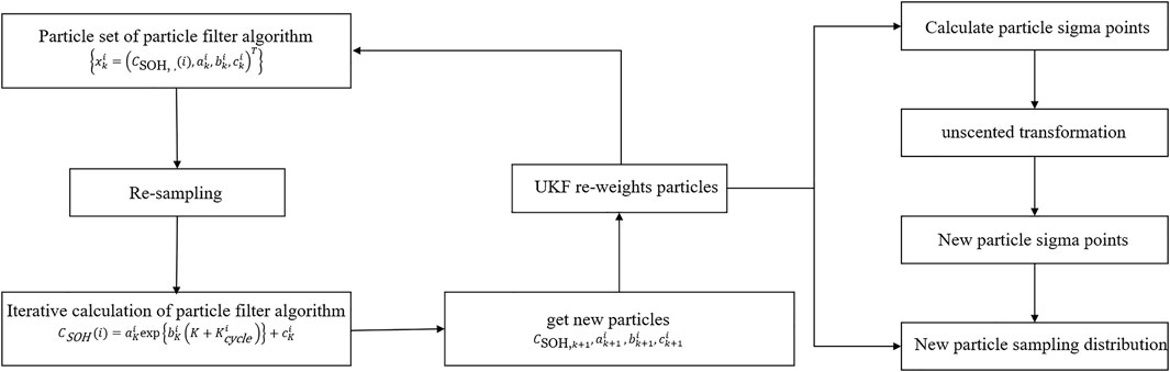
FIGURE 1. Flowchart of the fusion particle filter algorithm.

3.2 RUL Prediction Model Establishment

When a Li-ion battery undergoes continuous charge and discharge cycles, the actual capacity of the battery decreases exponentially with the number of cycles. Taking the lithium-ion battery cycle life empirical decay model as the state equation in the particle filter algorithm, it uses its excellent state tracking ability to determine the unknown parameters in the empirical model and finally realizes the prediction of the remaining battery life.

Assuming that the remaining life prediction cycle of the battery is k, the specific steps of the particle filter algorithm to predict the remaining life of the battery are as follows.

① Read battery SOH data during aging cycle;

② Use the recursive least-squares algorithm to fit the data from the initial cycle to the Kth cycle to determine the initial parameters a, b, and c of the single-exponential empirical model of life decay;

③Use the initial parameters of the empirical model and the battery SOH data from the initial cycle to the Kth cycle to perform the particle filter algorithm, update the adjusted particle set $\left\{x_k^i={\left(a_k^i,b_k^i,c_k^i\right)}^T\right\}$, ${\tilde{w}}_k^i$ in real time, and output the filtered battery SOH data value $C_{SOH}\left(i\right)$, where $i=\mathrm{1,2},\cdots ,K$;

④Predict the value $C_{SOH}\left(i\right)=a_K^i\exp \left\{b_K^i\left(K+K_{eccl}^i\right)\right\}+c_K^i$ of the $\left(K+1\right)$ th battery SOH from the particle set $\left\{x_k^i={\left(a_K^i,b_K^i,c_K^i\right)}^T\right\}$ of the Kth cycle, where $i=\mathrm{1,2},\cdots ,K$ and $C_{SOH}\left(K+1\right)$, while updating the particle set $\left\{x_{k+1}^i={\left(a_{K+1}^i,b_{K+1}^i,c_{K+1}^i\right)}^T\right\}$, where $i=\mathrm{1,2},\cdots ,K,K+1$;

⑤Continue to calculate until the battery SOH value $C_{SOH}\le 80\text{\%}$, anf output the corresponding $K_{cycle, end}$; the probability density distribution of remaining cycle life is obtained (39).

Then, the estimated remaining cycle life predicted at the Kth cycle is:

$K_{\mathrm{cycle},\mathrm{end}}\approx {\displaystyle \sum _{i=1}^N{w}_k^i{K}_{\mathrm{cycle} }^i}.(39)$

4 Lithium-Ion Battery Cycle Life Prediction Experiment and Analysis

4.1 Test Objects

In this article, the battery of type 18650 was selected as the research object, and the battery parameters are shown in Table 1. Also, the same batch of batteries was selected for cyclic aging experiments. Considering that the batteries mostly work in the vicinity of 0–30°C under actual conditions, the cyclic aging test was performed at two temperatures (20°C and 30°C, respectively). In the cyclic aging experiment, the discharge rate was 1C and 2C for constant current discharge, respectively, and the charge rate of 0.5C was uniformly used for constant current charging during charging, and there was no constant voltage stage. The battery charging and discharging equipment used was ARBIN 2000, and the temperature of the battery during the experiment was controlled using an incubator.

TABLE 1

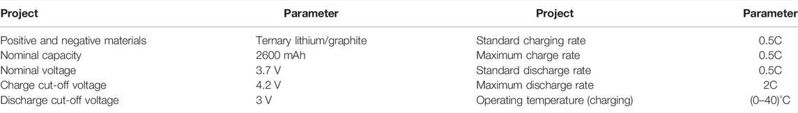
TABLE 1. Parameters of domestic 18650 battery.

Considering the influence of charge–discharge rate and ambient temperature on the aging rate of the battery in the cyclic aging experiment, in order to obtain the real maximum usable capacity of the battery, the capacity of the No. 1 to No. 4 batteries was tested after a certain number of cycles during the experiment. Among them, No. 1 and No. 2 batteries were tested for capacity once every 20 charge–discharge cycles, No. 3 battery was tested once every 15 cycles, and No. 4 battery was tested once every 10 cycles. The capacity test was to let the battery stand for 1 h after charging, then discharge at a constant current with a discharge rate of 0.1C until the discharge cut-off voltage was 2.4 V, and finally the battery capacity at this point was recorded.

4.2 Experimental Comparison and Result Analysis

The particle filter algorithm is used to predict the remaining service life of the lithium-ion battery, and the simulation results are shown in Figures 2–5. As can be seen from Table 2, there were different starting points for prediction, the more data that can be used as a reference battery capacity decay sample, the more accurately the particle filter algorithm can track the decay trend and optimize the parameters in the capacity decay empirical model. The accuracy of predicting remaining useful life also improved. It can be seen that the remaining service life of the battery is predicted at different prediction starting points, and the prediction error would gradually decrease with the increase of the known capacity data.

FIGURE 2

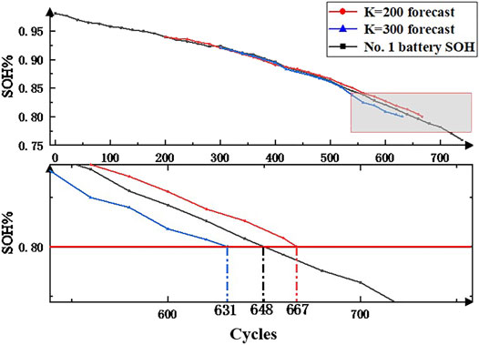
FIGURE 2. Prediction results of the particle filter algorithm for No. 1 battery.

FIGURE 3

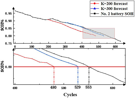
FIGURE 3. Prediction results of the particle filter algorithm for No. 2 battery.

FIGURE 4

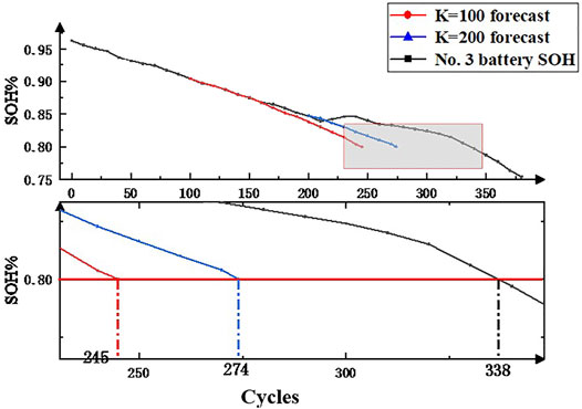
FIGURE 4. Prediction results of the particle filter algorithm for No. 3 battery.

FIGURE 5

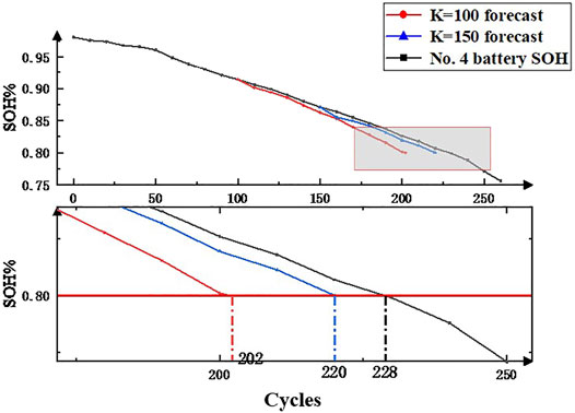
FIGURE 5. Prediction results of the particle filter algorithm for No. 4 battery.

TABLE 2

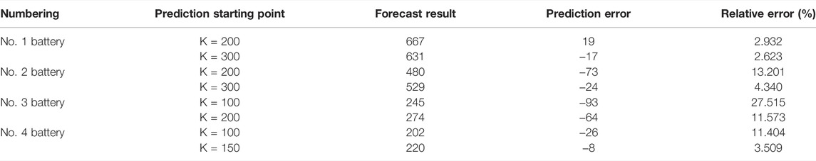
TABLE 2. Prediction results of the particle filter algorithm for batteries 1–4.

Analysis of the relative error of more than 10% in the table shows that the SOH decline process of the battery did not always decrease with the increase of the number of cycles. In the process of SOH decay of No. 2–4 batteries, the SOH of the battery would rise or not change for a period of time. This also means that the more complete the data that can be used as a reference battery capacity degradation sample, the more accurately the particle filter algorithm can predict the remaining life of the battery.

The relative error of No. 4 battery exceeded 10% when K = 100, but the relative error was only 3.5% when K = 150. At this time, the difference between the reference samples was only 50 copies. It can be observed from Figures 2–5 that the No. 4 battery has a period of flat SOH near the 50th cycle, and the proportion of this stage in the first 100 cycles must be greater than the proportion of the first 150 cycles. This stage has a greater impact on the prediction when K = 100, resulting in an inaccurate prediction. But the same situation also happened with the No. 2 battery. When the No. 2 battery started prediction at K = 300, the SOH of the battery first increased and then decreased between 200 and 250 cycles. However, in the end, the prediction error of the No. 2 battery at K = 300 was only 24 times, and the relative error was only 4.3%, so the prediction was more accurate.

In Table 3, as the number of reference samples increases, the PDF width of the prediction results also decreases. When K = 100, the width is 21, and when K = 300, the width drops to 11. From this, it can also be shown that the more the reference samples, the higher the accuracy of the prediction results. It can be seen from Table 3 that the prediction result given by the particle filter algorithm is a range, which realizes the quantitative expression of the uncertainty of the RUL prediction result of the lithium-ion battery. It provides more scientific and reasonable information by giving the interval range and probability density distribution of the prediction results.

TABLE 3

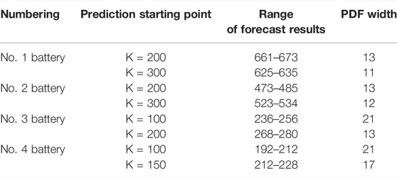
TABLE 3. Probability density distribution of predicted results of nos. 1–4 batteries.

It can be seen from the aforementioned analysis that in the whole life of the battery, the SOH that characterizes the life of the battery does not decrease with the increase of the number of cycles, but also has a flat and rising stage, but this stage is unpredictable and will eventually lead to fluctuations in the prediction results. In the particle filter algorithm, this is called singular value. At the same time, the particle filter algorithm also has problems such as particle degradation. In order to solve these problems, this article proposes an improved particle filter algorithm for optimization to improve the prediction accuracy.

The remaining service life of the lithium-ion battery is predicted by the improved particle filter algorithm, and the simulation results are shown in Figures 6–9. It can be observed in Table 4 that both prediction error and relative error compared with Table 2 have decreased, especially for battery 2 prediction starting point K = 200 and battery 4 prediction starting point K = 100; the relative error of these two decreases more obviously, where battery 2 K = 200 prediction relative error decreased from 13.2% to 1.6%, reduced by about 11%. Then we compared the prediction results of the improved particle filtering algorithm prediction experiment for battery 2 K = 300 with the prediction results of the particle filtering algorithm experiment for battery 2 K = 300 and found that the prediction error decreased from 24 cycles to 2 cycles and the relative error decreased from 4.34% to 0.36%.

FIGURE 6

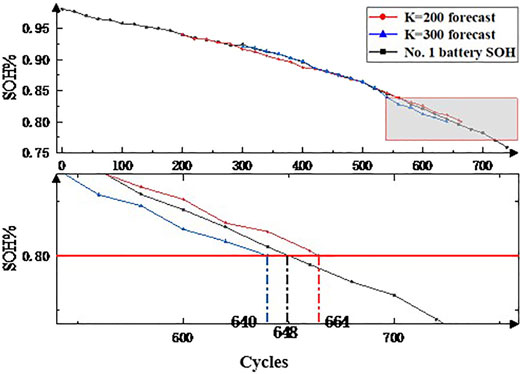
FIGURE 6. Prediction results of the improved particle filter algorithm for No. 1 battery.

FIGURE 7

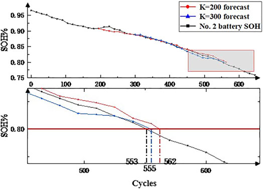
FIGURE 7. Prediction results of the improved particle filter algorithm for No. 2 battery.

FIGURE 8

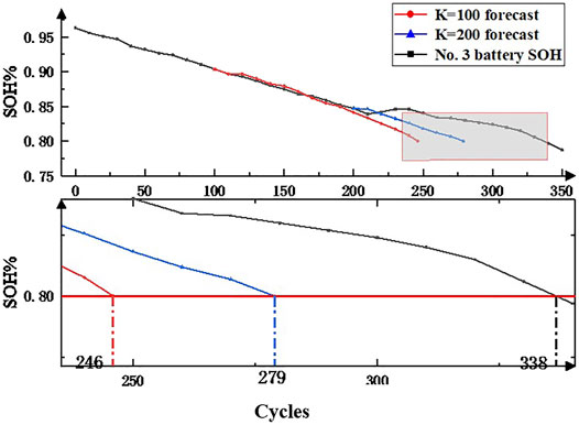
FIGURE 8. Prediction results of the improved particle filter algorithm for No. 3 battery.

FIGURE 9

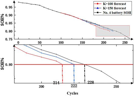
FIGURE 9. Prediction results of the improved particle filter algorithm for No. 4 battery.

TABLE 4

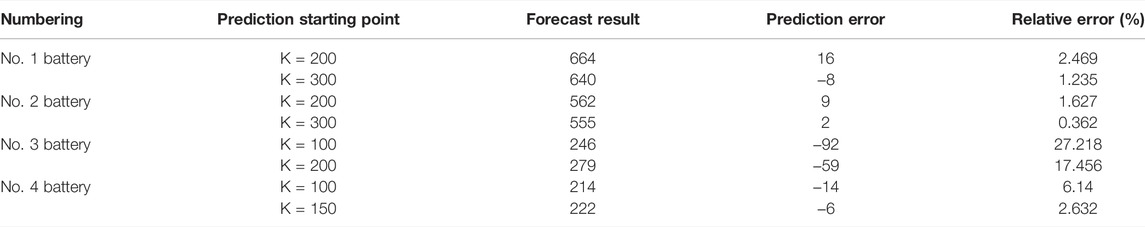
TABLE 4. Prediction results of the improved particle filter algorithm for batteries 1–4.

The particle filter algorithm obtained through the aforementioned analysis will be affected by the singular value. The analysis of the K = 300 prediction result of the No. 2 battery shows that the influence of the singular value on the singular value is indeed reduced after the introduction of the UKF algorithm. The same battery 4, which was affected by singular values in the particle filtering algorithm experiments leading to inaccurate prediction results, was improved in the improved particle filtering algorithm prediction experiments in K = 100 prediction results in the relative error decreased from 11.4% to 6.14%, and the prediction accuracy was improved. In this experiment, the singular values in the SOH decay curve of the No. 3 battery were not included in the reference sample, and the predicted results and relative errors of the No. 3 battery basically did not change.

The interval range and probability density distribution of the prediction results of the improved algorithm are shown in Table 5. As can be seen in Table 5, as the number of reference samples increases, the PDF width of the prediction results decreases. Compared with Table 3, when the number of reference samples is the same, the PDF width of the prediction results of the improved particle filter algorithm is slightly smaller than that of the particle filter algorithm, indicating that the fluctuation of the prediction results is smaller and the results are more accurate. In order to more intuitively discover the influence of singular values on the prediction results, the following subsections will conduct a separate experimental comparison.

TABLE 5

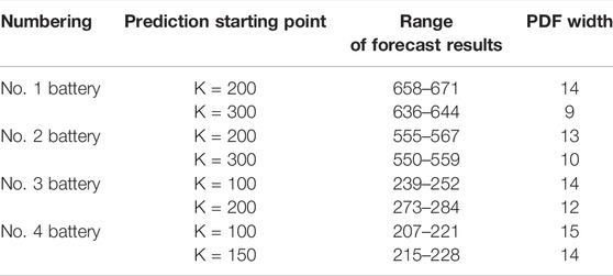
TABLE 5. Predicted probability distribution of batteries 1–4 by the improved particle filter algorithm.

4.3 Singular Value Comparison Experiment

In the aforementioned experiments, it was found that the singular value will have an impact on the prediction results. By introducing the UKF, it was found that the prediction results of the No. 2 and No. 4 batteries affected by the singular value in the experiment had been improved in the prediction experiment of the improved particle filter algorithm. In order to verify the suppression effect of the improved particle filter algorithm on singular values, the No. 3 battery was selected as the experimental target for comparative experiments.

Observing Figure 10, it can be found that when the prediction starting point is the 240th cycle, compared with the prediction curve obtained by the standard PF algorithm, the prediction curve obtained by the improved algorithm is closer to the capacity decay curve of the No. 3 battery. Both the prediction error and the relative error of the improved particle filter algorithm are lower than those of the previous particle filter algorithm, especially in the 310 to 360 cycles; the prediction results of the improved particle filter algorithm almost coincide with the actual results. It shows that the improved particle filter algorithm introduced with UKF is less affected by singular values.

FIGURE 10

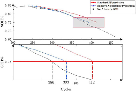
FIGURE 10. Singular value comparison experiment.

5 Conclusion

The RUL prediction of lithium-ion batteries plays an important role in PHM. Accurately predicting the RUL of lithium-ion batteries can improve the safety and reliability of the energy storage system. In this article, an improved particle filter RUL prediction method for lithium-ion batteries is proposed, which improves the filtering accuracy while ensuring the diversity of particles. Compared with the UKF algorithm or the PF algorithm alone, the improved particle filter algorithm proposed in this article can not only overcome the constraints of nonlinear systems but also reduce the influence of particle degradation and singular values on the estimation results, which has wider application prospects. From the experimental results given in Section 4.2, it can be seen that compared with the traditional PF algorithm, the improved algorithm has high accuracy and stability for battery RUL prediction. At the same time, as the starting point of the experimental prediction is moved back, better prediction results can be obtained by using more measured data. However, the proposed method still has some limitations. For example, the data used were obtained from an experimental environment, which is different from the actual working environment of the battery. How to accurately predict RUL in a working environment with uncertain environmental factors such as weather and road conditions remains to be further studied. In addition, the aforementioned degradation model is a strictly monotonic function, while the RUL degradation trend of some lithium-ion batteries is actually non-monotonic and exhibits strong volatility. Therefore, in the future PHM, a lot of research is needed to establish a more robust degradation model that can describe non-monotonic degradation trends, and more parameters will be used as indicators for management decision-making. The method for predicting the remaining service life proposed in this article aims to help users estimate the maximum usable performance of the battery and provide users with an accurate battery capacity estimate in advance, so that the user can make a decision whether or not to replace the battery.

Data Availability Statement

The original contributions presented in the study are included in the article/Supplementary Material, and further inquiries can be directed to the corresponding author.

Author Contributions

TZ: conceptualization, methodology, and writing—original draft. TW: writing—review and editing and supervision. SX: data curation.

Funding

This work is supported by the Hubei Provincial Major Technology Innovation Project of China (Grant No. 2018AAA056) and the National Natural Science Foundation of China (Grant No. 51677058).

Conflict of Interest

The authors declare that the research was conducted in the absence of any commercial or financial relationships that could be construed as a potential conflict of interest.

Publisher’s Note

All claims expressed in this article are solely those of the authors and do not necessarily represent those of their affiliated organizations, or those of the publisher, the editors, and the reviewers. Any product that may be evaluated in this article, or claim that may be made by its manufacturer, is not guaranteed or endorsed by the publisher.

References

Chang, Y., Fang, H., and Zhang, Y. (2017). A New Hybrid Method for the Prediction of the Remaining Useful Life of a Lithium-Ion Battery. Appl. Energy 206 (15), 1564–1578. doi:10.1016/j.apenergy.2017.09.106

CrossRef Full Text | Google Scholar

Chao, L., Quinzhi, L., and Tengfei, L. (2016). A Lead-Acid Battery's Remaining Useful Life Prediction by Using Electrochemical Model in the Particle Filtering Framework. Energy 120, 975.doi:10.1016/j.energy.2016.12.004

CrossRef Full Text | Google Scholar

Chen, Z., Yang, L., Zhao, X., Wang, Y., and He, Z. (2019). Online State of Charge Estimation of Li-Ion Battery Based on an Improved Unscented Kalman Filter Approach. Appl. Math. Model. 70, 532–544. doi:10.1016/j.apm.2019.01.031

CrossRef Full Text | Google Scholar

Duan, B., Zhang, Q., Geng, F., and Zhang, C. (2020). Remaining Useful Life Prediction of Lithium‐ion Battery Based on Extended Kalman Particle Filter. Int. J. Energy Res. 44 (3), 1724–1734. doi:10.1002/er.5002

CrossRef Full Text | Google Scholar

Feng, F., Teng, S., Liu, K., Xie, J., Xie, Y., Liu, B., et al. (2020). Co-estimation of Lithium-Ion Battery State of Charge and State of Temperature Based on a Hybrid Electrochemical-Thermal-Neural-Network Model. J. Power Sources 455, 227935. doi:10.1016/j.jpowsour.2020.227935

CrossRef Full Text | Google Scholar

Hu, X., and Tang, X. (2018). Review of Modeling Techniques for Lithium-Ion Traction Batteries in Electric Vehicles. J. Mech. Eng. 16, 20. doi:10.3901/JME.2017.16.020

CrossRef Full Text | Google Scholar

Huangfu, Y., Xu, J., Zhao, D., Liu, Y., and Gao, F. (2018). A Novel Battery State of Charge Estimation Method Based on a Super-twisting Sliding Mode Observer. Energies 11, 1211. doi:10.3390/en11051211

CrossRef Full Text | Google Scholar

Li, X., Fan, G., Rizzoni, G., Canova, M., Zhu, C., and Wei, G. (2016). A Simplified Multi-Particle Model for Lithium Ion Batteries via a Predictor-Corrector Strategy and Quasi-Linearization. Energy 116, 154–169. doi:10.1016/j.energy.2016.09.099

CrossRef Full Text | Google Scholar

Li, Y., Vilathgamuwa, M., Farrell, T., Choi, S. S., Tran, N. T., and Teague, J. (2019). A Physics-Based Distributed-Parameter Equivalent Circuit Model for Lithium-Ion Batteries. Electrochimica Acta 299, 451–469. doi:10.1016/j.electacta.2018.12.167

CrossRef Full Text | Google Scholar

Liu, K., Hu, X., Wei, Z., Li, Y., and Jiang, Y. (2019a). Modified Gaussian Process Regression Models for Cyclic Capacity Prediction of Lithium-Ion Batteries. IEEE Trans. Transp. Electrific. 5, 1225–1236. doi:10.1109/TTE.2019.2944802

CrossRef Full Text | Google Scholar

Liu, K., Li, K., Peng, Q., and Zhang, C. (2019b). A Brief Review on Key Technologies in the Battery Management System of Electric Vehicles. Front. Mech. Eng. 14, 47–64. doi:10.1007/s11465-018-0516-8

CrossRef Full Text | Google Scholar

Liu, Z., Sun, G., Bu, S., Han, J., Tang, X., and Pecht, M. (2017). Particle Learning Framework for Estimating the Remaining Useful Life of Lithium-Ion Batteries. IEEE Trans. Instrum. Meas. 66 (2), 280–293. doi:10.1109/TIM.2016.2622838

CrossRef Full Text | Google Scholar

McTurk, P. E., Allerhand, M., Medina-Lopez, E., Anjos, M. F., Sylvester, J., and dos Reis, G. (2020). Identification and Machine Learning Prediction of Knee-point and Knee-Onset in Capacity Degradation Curves of Lithium-Ion Cells. Energy AI 1, 100006. doi:10.1016/j.egyai.2020.100006

CrossRef Full Text | Google Scholar

Nagulapati, V. M., Lee, H., Jung, D., S Paramanantham, S., Brigljevic, B., Choi, Y., et al. (2021). A Novel Combined Multi-Battery Dataset Based Approach for Enhanced Prediction Accuracy of Data Driven Prognostic Models in Capacity Estimation of Lithium Ion Batteries. Energy AI 5, 100089. doi:10.1016/j.egyai.2021.100089

CrossRef Full Text | Google Scholar

Patil, M. A., Tagade, P., Hariharan, K. S., Kolake, S. M., Song, T., Yeo, T., et al. (2015). A Novel Multistage Support Vector Machine Based Approach for Li Ion Battery Remaining Useful Life Estimation. Appl. Energy 159, 285–297. doi:10.1016/j.apenergy.2015.08.119

CrossRef Full Text | Google Scholar

Qian, Y., and Yan, R. (2015). Remaining Useful Life Prediction of Rolling Bearings Using an Enhanced Particle Filterlter. IEEE Trans. Instrum. Meas. 64, 2696–2707. doi:10.1109/TIM.2015.2427891

CrossRef Full Text | Google Scholar

Ren, L., Zhao, L., Hong, S., Zhao, S., Wang, H., and Zhang, L. (2018). Remaining Useful Life Prediction for Lithium-Ion Battery: A Deep Learning Approach. IEEE Access 6, 50587–50598. doi:10.1109/ACCESS.2018.2858856

CrossRef Full Text | Google Scholar

Saxena, S., Xing, Y., Kwon, D., and Pecht, M. (2019). Accelerated Degradation Model for C-Rate Loading of Lithium-Ion Batteries. Int. J. Electr. Power. Energy Syst. 107, 438–445. doi:10.1016/j.ijepes.2018.12.016

CrossRef Full Text | Google Scholar

Sbarufatti, C., Corbetta, M., Giglio, M., and Cadini, F. (2017). Adaptive Prognosis of Lithium-Ion Batteries Based on the Combination of Particle Filters and Radial Basis Function Neural Networksfilters and Radial Basis Function Neural Networks. J. Power Sources 344, 128–140. doi:10.1016/j.jpowsour.2017.01.105

CrossRef Full Text | Google Scholar

Si, X.-S., (2015). An Adaptive Prognostic Approach via Nonlinear Degradation Modeling: Application to Battery Data. IEEE Trans. Ind. Electron. 62 (8), 5082–5096. doi:10.1007/978-3-662-54030-5_910.1109/tie.2015.2393840

CrossRef Full Text | Google Scholar

Wang, D., Yang, F., Tsui, K.-L., Zhou, Q., and Bae, S. J. (2016). Remaining Useful Life Prediction of Lithium-Ion Batteries Based on Spherical Cubature Particle Filterfilter. IEEE Trans. Instrum. Meas. 65 (6), 1282–1291. doi:10.1109/tim.2016.2534258

CrossRef Full Text | Google Scholar

Wang, F.-K., and Mamo, T. (2018). A Hybrid Model Based on Support Vector Regression and Differential Evolution for Remaining Useful Lifetime Prediction of Lithium-Ion Batteries. J. Power Sources 401, 49–54. doi:10.1016/j.jpowsour.2018.08.073

CrossRef Full Text | Google Scholar

Wang, H., Song, W., Zio, E., Kudreyko, A., and Zhang, Y. (2020). Remaining Useful Life Prediction for Lithium-Ion Batteries Using Fractional Brownian Motion and Fruit-Fly Optimization Algorithm. Measurement 161, 107904. doi:10.1016/j.measurement.2020.107904

CrossRef Full Text | Google Scholar

Wang, Y., Tian, J., Sun, Z., Wang, L., Xu, R., Li, M., et al. (2020). A Comprehensive Review of Battery Modeling and State Estimation Approaches for Advanced Battery Management Systems. Renew. Sustain. Energy Rev. 131, 110015. doi:10.1016/j.rser.2020.110015

CrossRef Full Text | Google Scholar

Wang, Y., Wang, L., Li, M., and Chen, Z. (2020). A Review of Key Issues for Control and Management in Battery and Ultra-capacitor Hybrid Energy Storage Systems. eTransportation 4, 100064. doi:10.1016/j.etran.2020.100064

CrossRef Full Text | Google Scholar

Wu, J., Zhang, C., and Chen, Z. (2016). An Online Method for Lithium-Ion Battery Remaining Useful Life Estimation Using Importance Sampling and Neural Networks. Appl. Energy 173, 134–140. doi:10.1016/j.apenergy.2016.04.057

CrossRef Full Text | Google Scholar

Zhang, Y., Tang, Q., Zhang, Y., Wang, J., Stimming, U., and Lee, A. A. (2020). Identifying Degradation Patterns of Lithium Ion Batteries from Impedance Spectroscopy Using Machine Learning. Nat. Commun. 11, 1706. doi:10.1038/s41467-020-15235-7

PubMed Abstract | CrossRef Full Text | Google Scholar

Zhao, Y., Liu, P., Wang, Z., Zhang, L., and Hong, J. (2017). Fault and Defect Diagnosis of Battery for Electric Vehicles Based on Big Data Analysis Methods. Appl. Energy 207, 354–362. doi:10.1016/j.apenergy.2017.05.139

CrossRef Full Text | Google Scholar

Zhao, Y., Stein, P., Bai, Y., Al-Siraj, M., Yang, Y., and Xu, B.-X. (2019). A Review on Modeling of Electro-Chemo-Mechanics in Lithium-Ion Batteries. J. Power Sources 413, 259–283. doi:10.1016/j.jpowsour.2018.12.011

CrossRef Full Text | Google Scholar

Zheng, Y., Ouyang, M., Han, X., Lu, L., and Li, J. (2018). Investigating the Error Sources of the Online State of Charge Estimation Methods for Lithium-Ion Batteries in Electric Vehicles. J. Power Sources 377, 161–188. doi:10.1016/j.jpowsour.2017.11.094

CrossRef Full Text | Google Scholar