Coot Algorithm for Optimal Carbon–Energy Combined Flow of Power Grid With Aluminum Plants

To achieve a low-carbon and economical operation for the power grid, this paper proposes a novel optimal carbon–energy combined flow (OCECF) by considering the influence of aluminum plants. It attempts to minimize the carbon emission of power grid, power loss, and the voltage deviation by taking the reactive power control of aluminum plants into account. Since the presented OCECF is a nonlinear and complex optimization problem, a new metaheuristic algorithm called Coot algorithm is employed to acquire a high-quality dispatch solution under various scenarios. The Coot algorithm is inspired by the movement of birds on the water surface, which can implement a wide exploration via the random movement and a deep exploitation via the chain movement with the group leaders. The performance of Coot algorithm for the presented OCECF is carried out on an IEEE 57-bus system with various power plants, in which the group search optimizer is introduced for performance comparison.

1 Introduction

In recent years, atypical weather patterns have resulted in the frequency of natural disasters, such as earthquake, flooding, and forest fires in the world, which directly related to the increasing production of carbon dioxide (CO₂) (Walther et al., 2002). The global temperature is increasing year by year due to the increase in the content of greenhouse gases in the atmosphere, and these are mainly caused by human activities. Among them, carbon dioxide is the most distinctive greenhouse gas. It shows that with the rapid development of the industry, environmental problems are becoming more and more severe and pose a threat to human health at the same time. The advocacy of low carbon life becomes inevitable, and the reduction in CO₂ has attracted extensive attention in both industry and research. In such a low-carbon–energy transition era, electric power industry, as a prime CO₂ producer, takes on greater responsibility for reducing carbon emissions from the generation side of electricity and from transmission flows. A lot of investigations have been concentrated on low-carbon electric power. From the point of view of environmental economy, clean energy technologies, such as carbon capture and storage technologies are key to reducing emissions in the current scenario where the power sector relies on emission-intensive energy resources (Wei et al., 2016). In Ghorbani (2016), Song et al. proposed nonconvex planning for economic scheduling of CHP in various integrated cogeneration systems using exchange market algorithms. Power grid companies have been trying to find more reasonable resource dispatching solutions to rationally allocate power resources according to customer demand and optimize the distribution system to achieve the most economical and quality system operation (Carpentier et al., 1996). Liu et al. (2014) proposed a multistage scenario tree-based approach, which uses a rolling scheduling scheme to consider the uncertainty of solar energy, nondispatchable power, and thermal loads in the operation of building energy systems using uncertainty information updated every hour.

Due to the difference in emission levels, carbon emissions are bound to the scheduling process by imposing penalties on carbon generation. However, the existing penalty methods are still inadequate. A penalty-based approach to resource scheduling, minimizing the cost of carbon emissions penalties/environmental loss, is proposed in Liu et al. (2014) to allocate switching states and power distribution. Existing studies aim to reduce the generation of total carbon emissions and ignore the carbon emissions of the electricity network, which is closely related to the interests of the grid companies. To effectively deal with this challenge, an optimal carbon–energy combined flow (OCECF) for electricity networks was suggested in Kang et al. (2012), Li et al. (2013), Zhang et al. (2015), and Zhang et al. (2018), where the tracking method identifies carbon liability with full electricity consumer responsibility. The literature (Lassagne et al., 2013) shows that in industrial processes, such as aluminum production, it has been observed that the CO₂ levels in the fume capture the economic variability of the equipment. Moreover, due to the inherent characteristics of the wastewater generated by virgin aluminum refinery, the present methods of carbon trapping technology cannot be used directly. Therefore, studies have shown that it cannot be applied to the measurement of CO₂ emissions from power networks, including aluminum plants. Aluminum plants have some typical characteristics, such as heavy load and reactive voltage regulation demand, which should be factored into the OCECF. OCECF is a model characterized by nonlinear programming with multivariate and complex constraints. It usually has two techniques, namely, traditional optimization methods, heuristic algorithms, and metaheuristic algorithms. Traditional optimization algorithms like mixed-integer linear programming (Gan et al., 2019), De Casteljau’s algorithm (Zhou et al., 2021a), and reduced event-base algorithm (Zhou et al., 2021b) rely mainly on the precise magnetic pattern of a particular optimum, and it can easily fall into a local optimum for nonlinear multipole planning with noncontinuous features and restraints. In comparison, the metaheuristic algorithm Coot algorithm can have better performance than the heuristic algorithm, such as faster convergence and more accurate characteristics. A new krill swarm was proposed in Adhvaryyu et al. (2017), which was successfully applied to dynamic optimum energy tracking for combined heating and power systems. In Abbas et al. (2017), G. Abbas et al. discuss in detail various hybrid forms of particle swarm algorithms and perform in-depth nonconvex economic scheduling based on particle swarm optimization. Genetic algorithms are applied to microgrids, and a genetic algorithm-based optimizer is designed for the economic dispatch of microgrids with renewable energy sources. The metaheuristic algorithm is a stochastic algorithm for finding the best response.

A classification of optimality methods and approximation algorithms is made into two categories: precise and proximate algorithms. Precise algorithms are able to find the best answer accurately. However, they are inefficient sufficiently for demanding optimality issues, and their implementation duration grows exponentially with the dimension of the problem. Proximate algorithms are able to identify close to optimal solutions for rigorous optimization problems in a relatively short period of time. The development of metaheuristic algorithms was motivated by biological processes, the behavior of animals, and the concept of conservation and human activity. Based on the collective behavior of birds, a new optimization algorithm, Coot, simulates the movement of cores on water with a metaheuristic algorithm applied to the OCECF model in this paper, which has a better performance for power grid containing aluminum plants.

The next section of this article is structured as described below: The Numerical simulation of optimal carbon–energy combined flow Section 2 describes the numerical simulation of the OCECF with the participation of the aluminum plants. The Coot optimization algorithms for optimal carbon–energy combined flow Section 3 describes the basic principles of the Coot algorithm. The Design of Coot for optimal carbon–energy combined flow Section 3.3 develops the design of the Coot algorithm for OCECF, and the Case studies Section 4 presents the simulation results of the Coot algorithm for the constructed problem. Last, the Conclusion Section 5 draws the conclusion of this article.

2 Numerical simulation of optimal carbon–energy combined flow

2.1 Carbon–energy combined flow

In the existing studies, the carbon emission statistics are usually obtained by converting primary energy consumption to macroscopic statistics. These methods cannot reveal the characteristics of carbon emissions in power systems, and there are many limitations in their application. The concept of power system carbon emission flow in Figure 1 is proposed to combine carbon emission analysis with power system tide calculation, which provides new ideas for the research in the field of low carbon power. A power system carbon stream is defined as a virtual network stream that is dependent on the power tide and is used to characterize the carbon characteristics of electric power systems that maintain the tide in either path (Kang et al., 2012). For carbon flows, not only do factors such as grid topology, generator output power, and nodal power demand fluctuate, but they are notably driven by the carbon intensity of the generators and the shared liability between the power producers and the users of the energy. The calculation of CO₂ flow is based mainly on the obtained tide of the power system, where the carbon emissions of the entire electrical system are equivalent to the CO₂ emissions of the generation side C_P. Therefore, it can be described as the accumulation of the grid losses C_loss and demand-side carbon emissions C_d, as described below:

$C_{\text{P}}={\displaystyle \sum }_{w\in W}{P}_w{\delta }_w=C_{\text{d}}+C_{\text{loss}}(1)$

where Pw in the formula represents the delivery power of the wth generator, δw means the carbon emission intensity of the wth generator, and W is the total generator set.

FIGURE 1

FIGURE 1. Joint carbon–energy flows in electricity networks.

Theoretically, electricity producers, i.e., power generators as well as grid companies, are primarily concerned with their own carbon emission quantities and footprints (Liu et al., 2014). For electricity users and consumers, they are concerned with the amount of their own carbon emissions. Therefore, analyzing only the first two will inevitably lead to multiple calculations of carbon emissions, lacking consideration of the co-responsibility component. To better refine this issue, the shared responsibility algorithm appropriately decomposes the overall carbon emissions of electricity producers and consumers as described below:

$C_{\text{p}}=\left(1-{\alpha }_{\text{p}}\right)C_{\text{e}}+{\alpha }_{\text{p}}{C}_{\text{loss}}+\left(1-{\beta }_{\text{C}}\right){\alpha }_{\text{p}}{C}_L+{\alpha }_{\text{p}}{\beta }_C{C}_{\text{L}}(2)$

where αP is the share of the producer responsibility, and the value of αP is between 0 and 1. This means that it is not the party producing the electricity that is responsible for all the carbon emissions; only the αP portion is accounted for, and βC represents the share of the consumer responsibility, 0 < βC < 1. Similarly, the party that uses the electricity load is not only responsible for its own carbon emissions from electricity use but also shares a portion βC of the carbon emissions used for electricity production.

As the grid company, the first priority is to focus on energy and flow through tidal analysis, as well as functional energy power losses along with an obligation for carbon emissions associated with carbon flows. The power losses can be described as described below:

$P_{\text{loss}}={\displaystyle \sum }_{i,j\in N_{\text{L}}}{g}_{ij}\left[V_i^2+V_j^2-2V_i{V}_{j}cos{\theta }_{ij}\right](3)$

where Vi and Vj denote the size between the voltage of the ith and jth nodes, and gij represents the electrical conductivity of line i − j; θij means the variation of voltage phasor angle (node i and j), and NL shows the branch set.

Therefore, the power network companies also have a corresponding carbon emission duty Cpgc, which could be calculated according to (2):

$C_{\text{pgc}}={\alpha }_{\text{p}}{C}_{\text{loss}}+(1-{\beta }_{\text{C}}){\alpha }_{\text{p}}{C}_{\text{L}}(4)$

where C_loss needs to be calculated based on the proportionate allocation rule to obtain, and the proportional sharing principle can be shown as follows:

$C_{\text{ds}}={\displaystyle \sum }_{i,j\in N_{\text{L}}}{\displaystyle \sum }_{w\in W}\left(\frac{{\alpha }_{jw}^{(-1)}\Delta P_{ij}}{P_j^{\prime }}\right)P_w{\delta }_w(5)$

where ajw (−1) is convenient to depict the power coefficient of energy maps between the jth node and wth generator, Pij and Pj’ indicate the functional energy power losses of line i − j and the gross power flow of the jth node in the equivalent lossless grid separately.

2.2 Optimal carbon–energy combined flow model

There are several factors affecting the combined flow of carbon–energy, the strongest of which are functional energy power dispatch and redundant power scheduling (Zhang et al., 2015). Among them, functional energy power dispatch is decided by electricity generators, network utilities, and power clients; redundant power scheduling is mainly manipulated by power network companies. Hence, the OCECF model is described by the reactive power dispatch after the functional energy power dispatch, while minimizing their own carbon liabilities, functional energy power losses, and voltage deviations, where the aim feature could be expressed by a nonlinear weighting approach, as shown below:

$minf\left(x\right)={\mu }_1{P}_{\text{loss}}+{\mu }_2{C}_{pgc}+{\mu }_3{V}_{\text{d}}(6)$

subject to

$\{\begin{array}{c}{P}_{Gi}-P_{Di}-V_i{\displaystyle \sum }_{j\in N_i}{V}_j\left(g_{ij}\cos {\theta }_{ij}+b_{ij}\sin {\theta }_{ij}\right)=0\\ Q_{Gi}-Q_{Di}-V_i{\displaystyle \sum }_{j\in N_i}{V}_j\left(g_{ij}\cos {\theta }_{ij}-b_{ij}\sin {\theta }_{ij}\right)=0\\ Q_{Gi}^{\min }\le Q_{Gi}\le Q_{Gi}^{\max },i\in N_G\\ V_{Ci}^{\min }\le V_i\le V_{Ci}^{\max },i\in N_i\\ Q_{Ci}^{\min }\le Q_{Ci}\le Q_{Ci}^{\max },i\in N_C\\ T_k^{\min }\le T_k\le T_k^{\max },k\in N_T\\ \left|S_l\right|\le S_l^{\max },l\in N_L\end{array}(7)$

where x means the vector of the subsystem, which can substitute the voltage of the generator terminals, individual tapping location of the on-load tap-changer (OLTC) transformer, total number of capacitors and inductors connected, etc.; Vd means the voltage deviation index; μ1, μ2, and μ3 are corresponding weight factor to various targets, respectively, and each variable takes a value between 0 and 1, and the sum of the values of the three variables is 1.

The first two equations in Eq. (7) are the tidal balance codes, which can be used to constrain the active and reactive tidal balances as equations for the decentralized OCECF, in which PGi and QGi are the functional energy power and redundant power delivery of the ith node. The third and fourth equations in Eq. (7) are derived from the generator constraint equation, which means that the redundant power delivery and the generating busbar voltage are subject to their upper and lower limits. The fifth equation is the shunt capacitor constraint, since the reactive power compensation of controlled shunt capacitors can only run within their minimum and maximum limits, so, QCi describes the redundant power compensation of the ith node. Due to the tap position of the transformers being restricted by their minimum and maximum limits, so with the sixth formula in Eq. (7), Tk is the transformer tap ratio. So as to acquire secure functioning of all subsystems, the size of the voltage of the burden bus is limited by its lower limit, and the apparent power flow of each transmission line is limited by its upper limit, so with the last equation constraint in Eq. (7), and Sl stands for the power apparent on transmission line l. In the formula above, Ni is the node group, NG is the unit group, NC means the group of compensation facilities, NT means the tapped group of transformers, and NL means the group of the branches.

Besides, the deviation index of voltage can be described as below:

$V_{\text{d}}={\displaystyle \sum }_{i\in N_i}\left|\frac{2V_i-V_i^{max}-V_i^{min}}{V_i^{max}-V_i^{min}}\right| (8)$

2.3 Characteristics of aluminum plant load

As the second richest ingredient in the Earth’s capsule behind oxygen and silicon, aluminum is being used more and more widely in various fields with the rapid progress of modern chemical industry, agriculture, and science and technology (Cook et al., 2007). Since its special properties, aluminum has played a very crucial role in the flourishing of important industries, such as aviation, construction, and automobiles. So, it is essential to pay attention to the aluminum plant load.

The power supply system of an aluminum plant consists of four main components: transformer, motor, line, and load, and the load of an aluminum plant consists of two components: the power load as well as the electrolytic aluminum. The auxiliary facilities for aluminum electrolysis are mainly power loads. The power load is started before the aluminum electrolysis load is started, and the power load can only be stopped after the aluminum electrolysis load is withdrawn.

During normal operation, the aluminum electrolytic load cannot be quickly batched out in a short period of time. During the scheduled maintenance period of the electrolyzer, it is necessary to open and close the electrolyzer. In this case, it is inevitable to gradually reduce the current until the operation of short junctions begins and then to raise the current to normal values. In the planned maintenance of the electrolyzer, the time for opening and stopping it to operate its short-circuit position is not very long, but it is still necessary to ensure the continuity of a power plant-generating unit start-up as much as possible. There are some distinctive features of aluminum plant loads, such as large loads and high reactive voltage regulation requirements, so it is more important to take them into account in the OCECF model. Loads like the aluminum plant absorb reactive power from the grid and reduce the power factor. The low power factor increases not only the power loss in the power supply and distribution system but also the voltage loss and reduces the utilization rate of the power supply equipment. From Eqs. (9) and (10), it can be seen that providing reactive power compensation and reducing reactive power is an effective action to improve the power factor. Therefore, reactive power compensation devices must be used in a targeted manner to improve the power factor for such loads. The vector diagram in Figure 2 clearly demonstrates the need to provide reactive power compensation and improve the power factor.

$cos\phi =\frac{P}{S}=\frac{P}{\sqrt{P^2+Q^2}}(9)$

$cos\phi =\frac{P}{S}=\frac{P}{\sqrt{P^2+{\left(Q-Q\ast \right)}^2}}(10)$

FIGURE 2

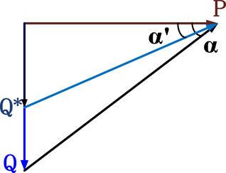
FIGURE 2. Vector diagram after reactive power compensation.

3 Coot optimization algorithms for optimal carbon–energy combined flow

3.1 Optimization principle

Coots are tiny fisher birds with numerous behaviors and maneuvers on the surface, as shown in Figure 3. As with the multiple leader PSO, it does not have a velocity argument. As a new evolutionary learning approach (Naruei and Keynia, 2021), the Coot algorithm has emerged from a study on them. The coots have diverse communal actions, and our aim in this document is to emulate group motion, i.e., both routine and nonroutine locomotion on the aquatic plane. The entire syndicate is guided toward the goal by the coot in front of the group and instructions from the coot ahead, which we define as the leader of the group. It has been found that coots have four separate motions on the aquatic surface, including random movement to this side and that side, chain movement, adjusting the position based on the group leaders, and leading the group by the leaders toward the optimal area (leader movement) (Memarzadeh and Keynia, 2021).

FIGURE 3

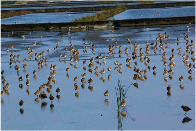
FIGURE 3. A chain of coots moving on the surface of the water.

The course of the procedure of the algorithm could be described in detail as below:

1) Initialization: A random population solution set is generated in the settlement field to form the primed population. The position of the ith Coot can be confirmed by Cootpos(i), and d is the set of decision variables. The minimum and maximum bounds of the specification variations are scheduled for ub and lb, and the equation can be shown as follows:

$\mathit{Cootpos}\left(i\right)=rand\left(1,\text{d}\right)\ast \left(ub-lb\right)+lb(11)$

After the initial overall is generated, the target problem is computed by comparing the objective function for each coot’s individual position. Meanwhile, N_L (number of leaders) and N_COOT (number of coots) are picked at random. The core of the algorithm is to look for the perfect coot or leader as holistically optimal at each step.

2) Position update: During the iterations, the coot’s location on the water is updated according to the four movements already mentioned above.

3.2 Four types of movement for coots

1) Random movement to this side and that side: In this motion, first, considering a stochastic location in the field of search and shift the coot to this stochastic location, named Q, is generated using formula (9). Besides, since the coot movement exploring many different sections of the field of the search, to prevent the result from getting stuck in a locally optimal position, formula (12) is used to update the position of the coot.

$\mathit{Cootpos}\left(i\right)=Cootpos\left(i\right)+A\ast R_2\ast \left(Q-Cootpos\left(i\right)\right)(12)$

where $R_2$ denotes a random number between 0 and 1, and A can be shown according to formula (13).

$A=1-iter\ast \left(\frac{1}{MaxIter}\right)(13)$

in which iter is the current iteration, and MaxIter denotes the maximum iteration.

2) Chain movement: There are two types of chain motion: one uses the even orientation of the two coots to achieve group motion, and another way to achieve chain motion is to first figure out the range of distance vector from two movers and shift it to another mover with a distance vector of about half. We used the first method, and the formula can be shown as follows:

$\mathit{Cootpos}\left(i\right)=0.5\text{∗}\left(Cootpos\left(i-1\right)+Cootpos\left(i\right)\right)(14)$

in which $\mathit{ Cootpos}\left(i-1\right)$ denotes the position of the second coot.

3) Adjusting the position based on the group leaders: Normally, the group is led by some coots’ group in front of it, and the rest of the coot must adjust their position according to the group leader and move closer to them, but a problem that may arise is that each coot adjusts its position according to the leader in the group. Therefore, it can be done by considering the average position of the leaders, and the coot updates its position according to this average position. Since considering the average position has the potential to lead to premature convergence, to achieve this movement, we use a mechanism to select leaders according to Eq. 15.

$\mathit{K}=1+\left(i MOD N_{\text{L}}\right)(15)$

where i denotes the reference value of the current coot, and K denotes the reference value of the leaders.

$\mathit{Cootpos}\left(i\right)=Leaderpos\left(k\right)+2\ast R1\ast COS\left(2R\pi \right)\ast \left(LeadersPos\left(k\right)-Cootpos\left(i\right)\right)(16)$

In Eq. 16, $\mathit{Cootpos}\left(i\right)$ shows the current position of coot; $\mathit{LeaderPos}\left(k\right)$ denotes the selected leaders’ position, R1 means a random number between 0 and 1, and R denotes a random number between −1 and 1.

4) Leading the group by the leaders toward the optimal area (leader movement): To direct the team to the target area, the optimal area, the leader needs to continually update their position on the target during the iterative process. The leader’s position can be better updated using Eq. (9). This formula is used to find a better position around the best position point of the current iteration around this current best point. There are some special cases where the leader must be made to move away from the current best position in order for the population to find a better position. Hence, the formula below provides a good way to approach the optimal position.

$\mathit{Leadrpos}\left(i\right)=\{\begin{array}{c}B\ast R3\ast \cos \left(2R\pi \right)\ast \left(gBest-LeaderPos\left(i\right)\right)+gBestR4<0.5\\ B\ast R3\ast \cos \left(2R\pi \right)\ast \left(gBest-LeaderPos\left(i\right)\right)-gBestR4\ge 0.5\end{array}(17)$

where gBest signs the optimal location of the ever iteration, random numbers R3 and R4 take values between 0 and 1, random number R is in the interval [−1,1], and B should be found based on formula (18).

$\mathit{B}=2-L\ast \left(\frac{1}{maxiter}\right)(18)$

A larger random motion can be generated by B*R3 in Eq. 17, preventing the algorithm from falling into a locally optimal solution set, while cos (2Rπ) is searched with different radii for a better location within this range around the region of best search. The question that tends to arise is how and when these various motions are shown. To guarantee the randomness of the optimization algorithm, all these movements we consider are random. This means that while the algorithm is being executed, the coots can move at random, in a chaining manner or toward the leader team.

3.3 Design of Coot for optimal carbon–energy combined flow

3.3.1 Fitness of coots and leaders

To obtain the desired result, minimizing the objective function 6) is the biggest goal. At the same time, each of the constraints in Eq. (7) needs to be satisfied. Therefore, a penalty function approach is used to design this fitness function as follows:

$Fit\left(x_j\right)={\mu }_1{P}_{\text{loss}}^j+{\mu }_2{C}_{\text{pgc}}^j+{\mu }_3{V}_{\text{d}}^j+\eta q^j,j\in J^e(19)$

in which $\eta$ denotes the punitive element, and q shows the amount of constraint breached inequalities.

3.3.2 Parameter setting

For the purpose of performing as desired for OCECF in Coot, several significant parameters, such as $P, N_{\text{L}},N_{\text{COOT}}, \text{and}MaxIter$, need to be carefully selected by analysis and calculation. A unified design was employed, and several exercises were conducted to ascertain the parameters, the optimum of which is shown in Table 1.

TABLE 1

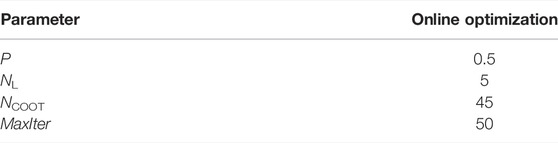
TABLE 1. The parameters used in Coot.

3.3.3 Execution procedure

Figure 4 outlines Coot’s overall execution procedure for OCECF.

FIGURE 4

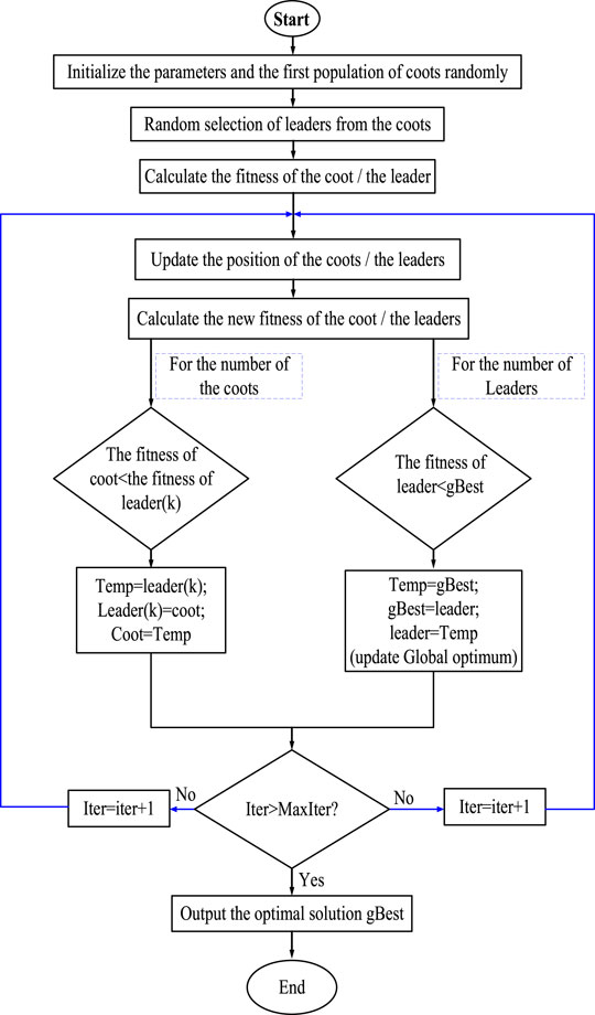
FIGURE 4. Coot flowchart of distributed optimal carbon–energy combined flow (OCECF).

4 Case studies

A common power system (IEEE 57 bus system in Figure 5) is selected as the benchmark system and evaluated by dynamic testing in this paper. For performance comparison, the classical heuristic optimization technique glowworm swarm optimization (GSO) algorithm was introduced in the study to perform experiments in OCECF. The simulations were carried out in Matlab R2019a, operated in a laptop with an Intel(R) Core TM i7 CPU with 3.8 GHz and 16 GB of RAM. According to the systematic analysis and research (Zhang et al., 2017), the shares of liability αp for producers and βc for consumers are each defined as 50% and 100%, respectively, to obtain relatively appropriate results. Overall, setting the same preference for each objective facilitates a better analysis, so it is a reasonable choice for the weighting coefficients (μ₁, μ₂, and μ₃) to be set to 1/3 on average. Assuming that the model OCECF is implemented in a 15-min cycle (Zhang et al., 2015), the mission count for 1 day is 96, and five of these typical nodes are selected for comparative analysis in the article.

FIGURE 5

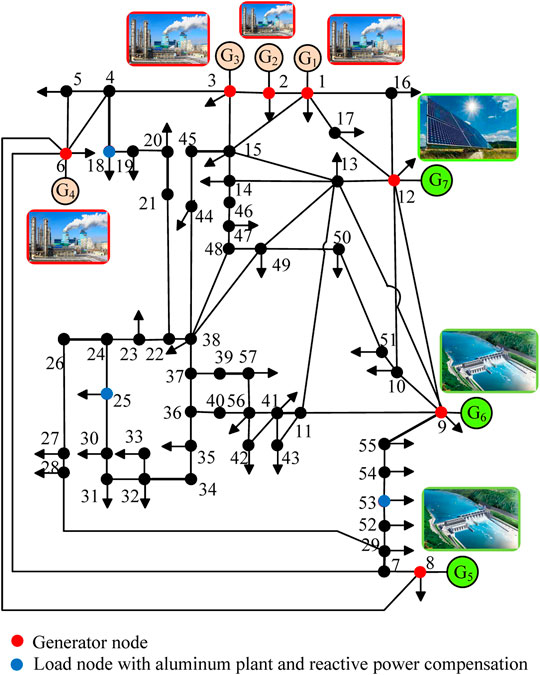
FIGURE 5. Topology of IEEE 57-bus system.

4.1 System model

The IEEE 57-bus system includes seven generators, and the carbon intensity δ_w for every single power producer is presented in Table 2. In addition, a detailed layout of the topology of the IEEE 57-bus system is supplied in Figure 7. The main parameters of regulation of the units are given in Table 1. Both the stock size of the algorithm and the maximal amount of the iterative strides were given to 50.

TABLE 2

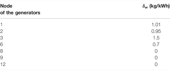
TABLE 2. CO₂ emission intensity of generators in IEEE 57-bus system.

4.2 Experiments and comparison

To help weigh the choice of algorithms in engineering applications, GSO, an algorithm with fast convergence and high-quality obtained solution sets, is introduced to test and compare the optimized performance online of Coot with the Coot algorithm proposed on the OCECF model. Compared with GSO, it is clearly described that Coot can acquire the most optimal and efficient approach toward the task due to its efficient exploitation. It is evident from the simulation plots that the GSO algorithm tends to fall into local optima, converges more slowly, and obtains worse fitness than Coot. This fully verifies the excellent global searching ability of Coot.

To evaluate the capability at the Coot operator, the online optimizing outputs of five conditions are compared in this example, as shown in Figures 6–11, where precision is used to approximate the simulation time for the actual regulated export and the curve of the regulating instructions. It is possible to notice that COOT has a significant empirical advantage compared with GSO. Table 3 shows the comparison of online optimization results under two different algorithms, while the optimal values of all the controllable variables are provided in Table 4. It can be found that COOT can acquire the smaller fitness function than GSO, thus, the voltage deviation, CO₂ exhaust, and electric consumption can be dramatically decreased.

FIGURE 6

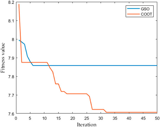
FIGURE 6. Comparison of algorithm simulation at a typical time node.

FIGURE 7

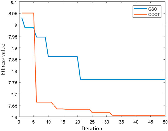
FIGURE 7. Comparison between coot and glowworm swarm optimization (GSO) for OCECF at 0:00.

FIGURE 8

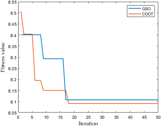
FIGURE 8. Comparison between coot and GSO for OCECF at 5:00.

FIGURE 9

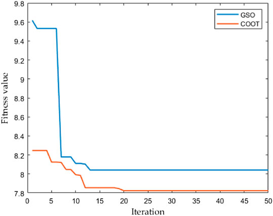
FIGURE 9. Comparison between coot and GSO for OCECF at 10:00.

FIGURE 10

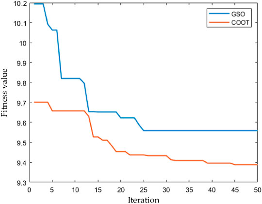
FIGURE 10. Comparison between coot and GSO for OCECF at 15:00.

FIGURE 11

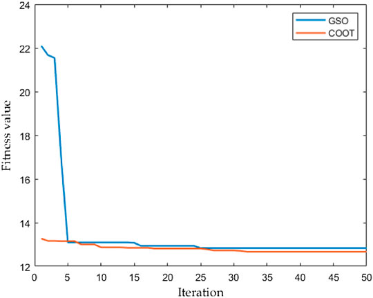
FIGURE 11. Comparison between coot and GSO for OCECF at 20:00.

TABLE 3

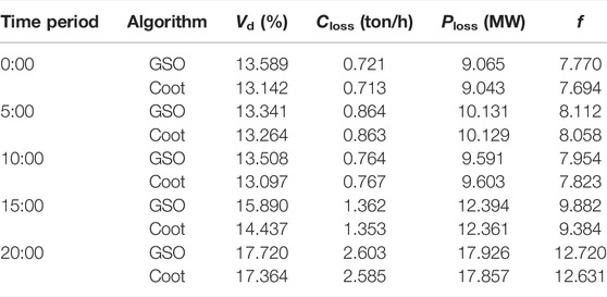
TABLE 3. Result comparison of online optimization under different algorithms at different times.

TABLE 4

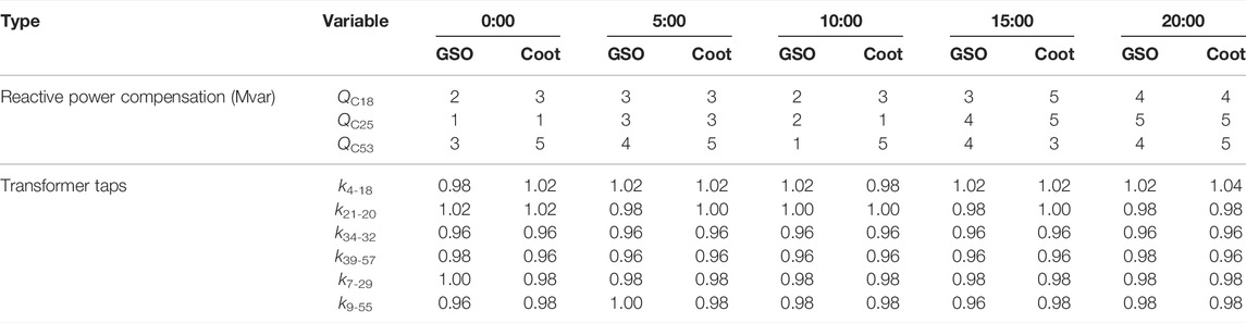
TABLE 4. Values of the optimal carbon–energy combined flow (OEOCF) model variables under two different algorithms in the IEEE 57-bus system.

5 Conclusion

In a nutshell, this study comprises the contribution of the following three aspects.

1) From a practical point of view, the constructed OCECF can take the participation of aluminum plants into account; thus, the CO₂ emission about the whole electricity supply system can be significantly reduced, especially on the part of the power grid.

2) A fast search algorithm for a solution set obtained by imitating the water movement of birds is applied to the model. Coot algorithm can implement a wide exploration via the random movement and a deep exploitation via the chain movement with the group leaders. Hence, a high-quality optimal solution can be acquired for OCECF.

3) It is confirmed from experiments that the Coot algorithm has more significant advantages in improving the convergence speed by an order of magnitude and guaranteeing the quality of the optimal solution compared with GSO.

Data Availability Statement

The original contributions presented in the study are included in the article/Supplementary Material. Further inquiries can be directed to the corresponding author.

Author Contributions

Conceptualization, LQ; Methodology, TX; Investigation, SL; Project administration, ZC; Resources, QZ; Formal analysis, JT; Supervision, YL; Writing—original draft, LQ.

Funding

This work is supported by research on carbon emission monitoring modeling method and low-carbon transformation strategy of key industries for carbon peaking and carbon neutrality goals (B704JY210069).

Conflict of Interest

LQ, TX, ZC, QZ, and JT are employed by the Economic Research Institute of State Grid Hebei Electric Power Company.

The remaining authors declare that the research was conducted in the absence of any commercial or financial relationships that could be construed as a potential conflict of interest.

Publisher’s Note

All claims expressed in this article are solely those of the authors and do not necessarily represent those of their affiliated organizations, or those of the publisher, the editors, and the reviewers. Any product that may be evaluated in this article, or claim that may be made by its manufacturer, is not guaranteed or endorsed by the publisher.

References

Abbas, G., Gu, J., Farooq, U., Raza, A., Asad, M. U., and El-Hawary, M. E. (2017). Solution of an Economic Dispatch Problem through Particle Swarm Optimization: A Detailed Survey - Part II. IEEE Access 5, 24426–24445. doi:10.1109/access.2017.2768522

CrossRef Full Text | Google Scholar

Adhvaryyu, P. K., Chattopadhyay, P. K., and Bhattacharya, A. (2017). Dynamic Optimal Power Flow of Combined Heat and Power System with Valve-point Effect Using Krill Herd Algorithm. Energy 127 (15), 756–767. doi:10.1016/j.energy.2017.03.046

CrossRef Full Text | Google Scholar

Carpentier, P., Gohen, G., Culioli, J.-C., and Renaud, A. (1996). Stochastic Optimization of Unit Commitment: A New Decomposition Framework. IEEE Trans. Power Syst. 11, 1067–1073. doi:10.1109/59.496196

CrossRef Full Text | Google Scholar

Cook, R., Chang, I. T. H., and Falticeanu, C. L. (2007). Aluminium and Aluminium alloy Powders for P/M Applications. MSF 534-536, 773–776. doi:10.4028/www.scientific.net/msf.534-536.773

CrossRef Full Text | Google Scholar

Gan, W., Ai, X., Fang, J., Yan, M., Yao, W., Zuo, W., et al. (2019). Security Constrained Co-planning of Transmission Expansion and Energy Storage. Appl. Energ. 239, 383–394. doi:10.1016/j.apenergy.2019.01.192

CrossRef Full Text | Google Scholar

Ghorbani, N. (2016). Combined Heat and Power Economic Dispatch Using Exchange Market Algorithm. Int. J. Electr. Power Energ. Syst. 82, 58–66. doi:10.1016/j.ijepes.2016.03.004

CrossRef Full Text | Google Scholar

Kang, C., Zhou, T., Chen, Q., Xu, Q., Xia, Q., and Ji, Z. (2012). Carbon Emission Flow in Networks. Sci. Rep. 2, 479–226. doi:10.1038/srep00479

PubMed Abstract | CrossRef Full Text | Google Scholar

Lassagne, O., Gosselin, L., Désilets, M., and Iliuta, M. C. (2013). Techno-economic Study of CO2 Capture for Aluminum Primary Production for Different Electrolytic Cell Ventilation Rates. Chem. Eng. J. 230, 338–350. doi:10.1016/j.cej.2013.06.038

CrossRef Full Text | Google Scholar

Li, B., Song, Y., and Hu, Z. (2013). Carbon Flow Tracing Method for Assessment of Demand Side Carbon Emissions Obligation. IEEE Trans. Sustain. Energ. 4 (4), 1100–1107. doi:10.1109/tste.2013.2268642

CrossRef Full Text | Google Scholar

Liu, P., Fu, Y., and Kargarian marvasti, A. (2014). Multi-stage Stochastic Optimal Operation of Energy-Efficient Building with Combined Heat and Power System. Electr. Power Compon. Syst. 42, 327–338. doi:10.1080/15325008.2013.862324

CrossRef Full Text | Google Scholar

Memarzadeh, G., and Keynia, F. (2021). A New Optimal Energy Storage System Model for Wind Power Producers Based on Long Short Term Memory and Coot Bird Search Algorithm. Energy Storage 44, 103401. doi:10.1016/j.est.2021.103401

CrossRef Full Text | Google Scholar

Naruei, I., and Keynia, F. (2021). A New Optimization Method Based on Coot Bird Natural Life Model. Expert Syst. Appl. 183 (30), 115352. doi:10.1016/j.eswa.2021.115352

CrossRef Full Text | Google Scholar

Walther, G. R., Post, E., Convey, P., Menzel, A., Parmesan, C., Beebee, T. J., et al. (2002). Ecological Responses to Recent Climate Change. Nature 416, 389–395. doi:10.1038/416389a

PubMed Abstract | CrossRef Full Text | Google Scholar

Wei, W., Liu, F., Wang, J., Chen, L., Mei, S., and Yuan, T. (2016). Robust Environmental-Economic Dispatch Incorporating Wind Power Generation and Carbon Capture Plants. Appl. Energ. 183, 674–684. doi:10.1016/j.apenergy.2016.09.013

CrossRef Full Text | Google Scholar

Zhang, X., Yu, T., Yang, B., Zheng, L., and Huang, L. (2015). Approximate Ideal Multi-Objective Solution Q(λ) Learning for Optimal Carbon-Energy Combined-Flow in Multi-Energy Power Systems. Energ. Convers. Manage. 106, 543–556. doi:10.1016/j.enconman.2015.09.049

CrossRef Full Text | Google Scholar

Zhang, X., Chen, Y., Yu, T., Yang, B., Qu, K., and Mao, S. (2017). Equilibrium-inspired Multiagent Optimizer with Extreme Transfer Learning for Decentralized Optimal Carbon-Energy Combined-Flow of Large-Scale Power Systems. Appl. Energ. 189 (1), 157–176. doi:10.1016/j.apenergy.2016.12.080

CrossRef Full Text | Google Scholar

Zhang, X., Yu, T., Guo, L., Yang, B., and Chen, Y. (2018). Culture Evolution Learning for Optimal Carbon-Energy Combined-Flow. IEEE Access 6, 15521–15531. doi:10.1109/access.2018.2815547

CrossRef Full Text | Google Scholar

Zhou, B., Fang, J., Ai, X., Yao, W., and Wen, J. (2021). Flexibility-Enhanced Continuous-Time Scheduling of Power System under Wind Uncertainties. IEEE Trans. Sustain. Energ. 12 (4), 2306–2320. doi:10.1109/tste.2021.3089696

CrossRef Full Text | Google Scholar

Zhou, B., Fang, J., Ai, X., Yang, C., Yao, W., and Wen, J. (2021). Dynamic Var Reserve-Constrained Coordinated Scheduling of LCC-HVDC Receiving-End System Considering Contingencies and Wind Uncertainties. IEEE Trans. Sustain. Energ. 12 (1), 469–481. doi:10.1109/tste.2020.3006984

CrossRef Full Text | Google Scholar