 Jinchao Zhang
 Yufeng Zhou1
 Qian Zhang
 Xiang Wang
 Qiang Zhao
- 1Fundamental Science on Nuclear Safety and Simulation Technology Laboratory, College of Nuclear Science and Technology, Harbin Engineering University, Harbin, China
- 2Department of Physics, Laboratory for Advanced Nuclear Energy Theory and Applications, Zhejiang Institute of Modern Physics, Zhejiang University, Hangzhou, China
During loading pattern (LP) optimization and reactor design, a lot of time consumption spent on evaluation is one of the key issues. In order to solve this issue, the surrogate models are investigated in this paper. The convolutional neural network (CNN) and fully convolutional network (FCN) are adopted to predict the eigenvalue and the assembly-wise power distribution (PD) for a simplified pressurized water reactor (PWR) during depletion, respectively. For the eigenvalue prediction during depletion, the error in the begin of cycle (BOC) and middle of cycle (MOC) is higher than that in the end of cycle (EOC). For the BOC and MOC, the samples with discrepancy over 500 pcm are less than 1%, except four burnup points. For the EOC, the fraction of samples with error over 500 pcm is less than 1%. As for the error of assembly power, the average absolute error is on the same level for all test cases. The average absolute relative error in the center region and the peripheral region is higher than that in the inter-ring region. The prediction results indicate the capability of neural network to predict core parameters.
1 Introduction
One of the key issues during loading pattern (LP) optimization and reactor design is time consumption for evaluating millions of LPs. The purpose of evaluation is to give out the fitness of each LP, which is commonly represented by the core key parameters. The conventional evaluation method gives the fitness by executing core calculation repeatedly, and it is the main source of time consumption. Therefore, a surrogate model, which rapidly produces the core key parameters, is desired.
In the past research, the artificial neural network (ANN) has been used in predicting core key parameters. Due to the constraints of computing resources, earlier studies apply the multi-layer perceptron (MLP) as the prediction model. The linearized parameter or macro data in the core are used as the input. Early examples of research into the model include the prediction of power peak factor (Mazrou and Hamadouche, 2004; Souza and Moreira, 2006; Niknafs et al., 2010; Saber et al., 2015), eigenvalue (Mazrou and Hamadouche, 2004; Saber et al., 2015), departure from nucleate boiling ratio (Lee and Chang, 2003), and core reload program (Kim et al., 1993a; Kim et al., 1993b; Hedayat et al., 2009). However, previous studies with the MLP model have failed to find any link between the input data and the environment. Loss of spatial information is an inherent problem of MLP, which is caused by the linearization of input parameters.
Recently, researchers have shown an increased interest in predicting core key parameters with the convolutional neural network (CNN) (Krizhevsky et al., 2012). Unlike the MLP neural network, the CNN directly uses the information related to the problem as its input. In this way, the CNN avoids the inherent problem caused by the linearization of input parameters. Besides, the CNN uses the convolutional kernel as its base unit, which is beneficial to the learning of local features. Thus, in core parameter prediction, the CNN has a higher potential than the MLP, which is composed of dense layers. Surveys such as that conducted by Jang and Lee (2019) have shown that the CNN has higher accuracy than the conventional neural network, when they use the LP information as input to predict the peak factoring and cycle lengths. Further research (Jang and Lee, 2019) reveals that there is still some potential of the CNN model. When regularization and normalization are used, the prediction accuracy could be improved. Unlike Jang and Lee (2019) and Jang (2020), Zhang (2019) predicted the eigenvalue by the CNN with the assembly cross sections (XSs) as its input. The results indicate that the single freedom of XS as the input of the CNN has better performance than the multiple of that. In addition to lumped parameter prediction, Lee et al. (2019) used the macroscopic XSs as input and predicted the assembly-wise power distribution (PD). The results show that the CNN model has better performance for the problems similar to training data than the dissimilar problems. This phenomenon could be mitigated by the involvement of adversarial training data. Besides, the same padding setting is used to ensure the unchanged data size before and after through the convolutional layer. In the field of PD prediction, Whyte and Parks (2020) took the LP information as input to predict the pin-wise PD. Different from the former, they achieved PD prediction by reshaping normal CNN output to the LP size. However, to predict the PD by the CNN, the original network needs some special settings or changes. For example, Lee et al. (2019) involved the same padding setting. Whyte and Parks (2020) reshaped the normal output. To avoid further machinery, Long et al. (2015) designed a fully convolutional network (FCN) to achieve pixel-to-pixel prediction. For PD prediction, the pixel-to-pixel predicting process is similar to the conventional core calculation. They both use the pixel-like information as input and output. The main differences include two aspects. The first one is that the CNN uses the LP information as its input, while the core calculation uses the assembly XSs as its input. Another one is that the CNN predicts the PD by a neural network, while the core calculation gets it by solving partial differential equations. Therefore, the FCN is a natural choice for assembly-wise PD prediction with the LP information as its input. Zhang et al. (2020) modified the FCN to predict the PD and flux distribution with the assembly XSs as its input. Compared to the MLP, the FCN shows better performance. This research reveals that the FCN has potential in distributed parameter prediction. But there has been minimal investigation of predicting the PD with the FCN during depletion.
Therefore, in this study, the CNN and FCN are implemented to predict eigenvalue and assembly-wise PD during depletion, respectively. And a simplified PWR problem with 13 burnup points is used to assess the performance of the trained models. To simplify the input of the neural networks, we choose the single freedom as the model input. The LP is encoded as the index matrix to serve as input of the models.
The remainder of this paper is organized as follows. The methodology is introduced in Section 2. The numerical results are presented in Section 3. Finally, Section 4 gives conclusions.
2 Methodology
2.1 Computing Framework Based on Neural Network
In the evaluation process, the conventional method gets the eigenvalue and PD by performing core calculation. But the method used in this article predicts them with the CNN and FCN models. It is the main difference between this research and before. Neural network models are generated by training with the datasets. The general computing framework is shown in Figure 1, which comprises three parts:
(1) Dataset generation. First, multiple fuel assemblies with different enrichment fuel and burnable poison rod quality are designed and labeled with a unique ID. Second, the few-group constants are generated by lattice calculation with the Monte Carlo code Serpent (Leppänen et al., 2015). Third, the core LP is generated by the random method. Finally, the core calculation is performed with the in-house diffusion code to generate the training and validation datasets. The details are described in Section 2.2.
(2) Model training. For a neural network model, it achieves learning knowledge by adjusting the parameters in its network. The learning process is named training. The architecture of the network decides the degree of learning. In this study, the CNN and the FCN are adopted as prediction models. They are introduced in Section 2.3.
(3) Model verification. The verification is performed to verify the efficiency of the trained models. And Section 3 gives the results.
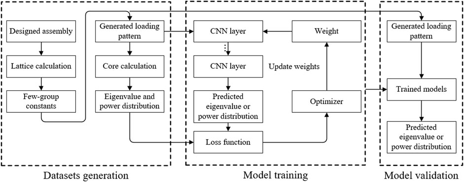
FIGURE 1. Computing framework of core parameter prediction.
2.2 Dataset Generation
The eigenvalue and the PD during burnup are determined by the initial LP. In this study, the reflector is fixed. The LP is randomly generated in a simplified PWR geometry in Figure 2, and the repetitive one will be abandoned. This generation process stops until the dataset size is reached. Then, the Serpent code is used to generate assembly few-group constants with the reflective boundary condition. Finally, the core calculation is performed with the in-house diffusion code for these LPs to obtain the eigenvalue and PD in each burnup point.
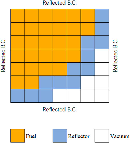
FIGURE 2. Geometry of the simplified PWR.
In order to preserve spatial information, the LP is encoded as a two-dimensional matrix, which is comprised of assembly IDs. Different assemblies have different fuel enrichments and burnable poison rod quantities. They include 25 enrichments varying from 12% to 18% divided into a constant interval of 0.25% and six different poison rod numbers including 0, 9, 13, 17, 21, and 25. The poison rods have the same 10B enrichment, which is 95%. Through the arrangement and combination of these settings, 150 different assemblies are formed. The temperature of the different problems is fixed as 900K. The fuel assembly is depleted to 100GWd/t, and the specific burnup steps are listed in Table 1. The basic power density of the fuel assembly is 0.5 MW/kg. In the designed assemblies, the moderator is fixed as the 561K water without the void and boron. The cladding material is fixed as the 600K stainless steel. The gap is fixed as 600K oxygen. The compositions of the above materials are given in Supplementary Appendix Table SA1. Figure 3 and Figure 4 describe the geometry of fuel assembly and the configuration of pin cell, respectively. As shown in Figure 3, there are four different groups of poison rod locations. For the assembly with nine poison rods, the location of the poison rod is marked with B1. For the assembly with thirteen poison rods, the poison rods are placed not only in B1 but also in B2. For the assembly with seventeen poison rods, the poison rods are placed in B1 and B3. For the assembly with twenty-one poison rods, the poison rods are placed in B1, B2, and B3. For the assembly with twenty-five poison rods, the poison rods are placed in B1, B3, and B4.

TABLE 1. Burnup points.
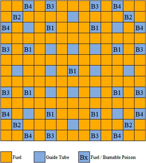
FIGURE 3. Assembly geometry.
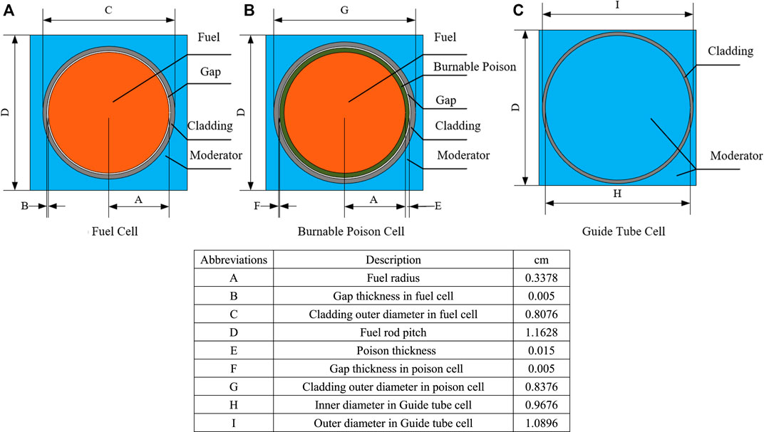
FIGURE 4. Geometry configuration of different cells.
In addition, considering that the eigenvalue in different burnup points is not prior data, the eigenvalue is not normalized.
2.3 Model Description
Different problems need different models with different architectures. In this study, two types of neural network models are used. We performed some primary sensitivity analysis on the network architectures used in this research. The results indicate that the current networks are the best. Any adjustment to them will worsen the prediction accuracy. Besides, it is difficult to find the law between the adjustment and the model performance. Thus, we do not report it in this manuscript. A complete sensitivity analysis of the network architecture requires a lot of iterations, which are difficult to complete in this research and are considered for the future. Then, the models used in this research are introduced. The first type is the CNN, which is adopted to predict the eigenvalue. Its structure comprises convolutional, pooling, and fully connected layers, which are shown in Supplementary Appendix Table SA2. The convolutional layer aims to take the spatial data into account. The pooling layer summarizes the feedback of the whole neighborhood and improves the efficiency of the network. The network finishes up with the fully connected layer, which connects the network and the object.
The second type is the FCN, which is a variant of CNN and is presented diagrammatically in Figure 5. It is noticed that, at the end of conventional CNN, several upsampling layers and concatenate layers are added to achieve backward stride convolution. They combine different feature layers and generate the output of corresponding size to the input. Thus, the FCN can predict the assembly-wise PD with the LP as its input. The FCN structure, which is adopted in this study, is shown in Supplementary Appendix Table SA3. Table 2 gives the parameters used in the above models.
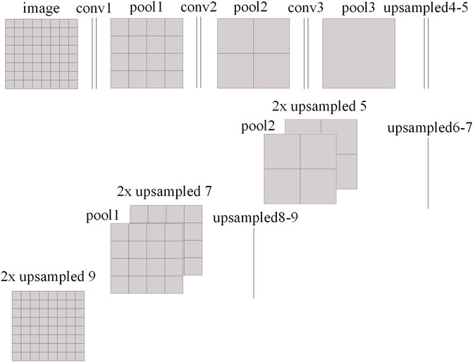
FIGURE 5. Schematic diagram of the FCN structure.
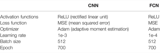
TABLE 2. Model parameters.
Furthermore, there are two points that need attention. First, the models with different burnup points are trained separately, which means that different burnup points have different neural networks. Second, due to the computational load for training 50 neural networks, this study chooses several representative burnup points. Thirteen burnup points are selected as representatives, including 0, 0.2, 0.5, 1.0, 2.0, 35.0, 37.5, 40.0, 42.5, 92.5, 95, 97.5, 100.0 GWd/t, which represent the begin of cycle (BOC), middle of cycle (MOC), and end of cycle (EOC).
In this study, the Keras framework (Chollet, 2015) is used to establish neural network structures upon TensorFlow. The CPU and GPU used in this work are 3.3 GHz Intel Core i9-7900X and Nvidia GeForce GTX 2080Ti, respectively.
3 Numerical Results
3.1 Eigenvalue Prediction
In this section, the CNNs are trained to predict the eigenvalue in different burnup points. The architecture shown in Supplementary Appendix Table SA2 was used. 1 million samples (0.8 million for training and 0.2 million for validation, with no overlap between the two datasets) were generated to train and validate the CNNs.
Figures 6–8 show the scattering plot of eigenvalue and the error distribution of predicted eigenvalue. In the scattering plot, the red line is the mean absolute error (MAE) ±500pcm. In the error distribution histogram, the black line is the normal distribution curve based on the prediction results. The σ symbol represents the standard deviation of error distribution. The green region, the blue region, the red region, and the black region are the normal distribution range of 1σ, 2σ, and 3σ and the region out of 3σ, respectively. Table 3 summarizes the detailed results.
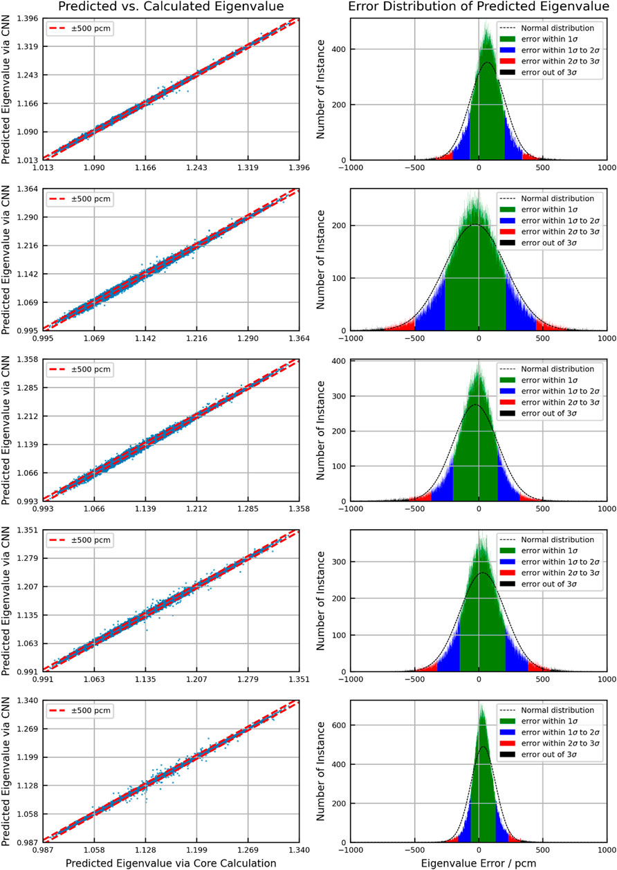
FIGURE 6. Eigenvalue predicted accuracy of the BOC.
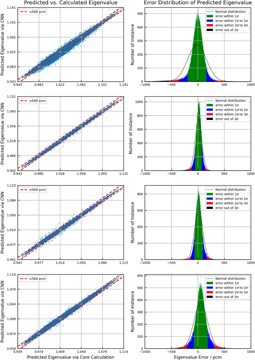
FIGURE 7. Eigenvalue predicted accuracy of the MOC.
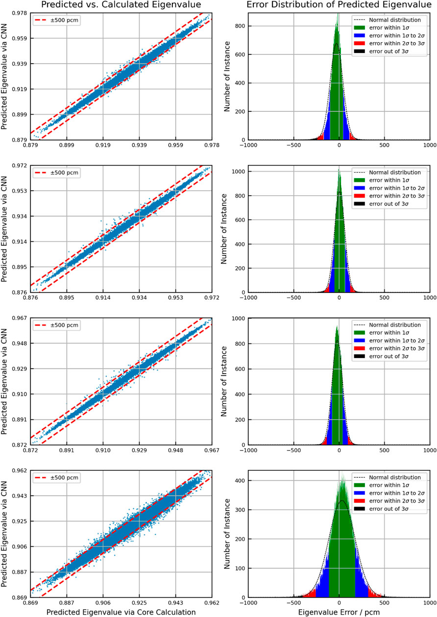
FIGURE 8. Eigenvalue predicted accuracy of the EOC.
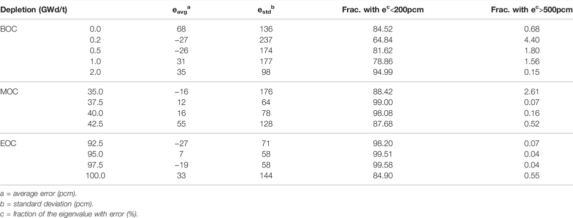
TABLE 3. Eigenvalue prediction error of trained models.
As a result of validation, in different burnup stages, the error distribution of the discrepancy between the predicted eigenvalue and the reference is close to normal distribution. However, compared to the normal distribution, the eigenvalue prediction error of CNN models is higher within the 1σ range. This means that the distribution of prediction error is more concentrated around the average error. But in the region of error exceeding 1σ, the distribution is wider than the normal distribution. The average error in all cases is within 100pcm. There is no obvious peak shift. Besides, the samples with the absolute error over 500 pcm are less than 3%, except for the second burnup point in the BOC. In general, the error in the BOC and MOC is higher than that in the EOC. This is because the reactivity of different assemblies varies greatly with poison depletion, which is greatly affected by the location. It increases the difficulty of the prediction process.
3.2 Power Distribution Prediction
As a further test of neural network, the FCNs are trained to predict PD. The architecture, shown in Supplementary Appendix Table SA3, was used. 1 million PD samples, generated with the eigenvalue, were used to train and validate the FCNs.
For the relative power of each assembly in different burnup stages, Figures 9–11 give the assembly average power, the assembly average absolute error, and the average value of the absolute relative error. The color of figures is given according to the assembly average power.
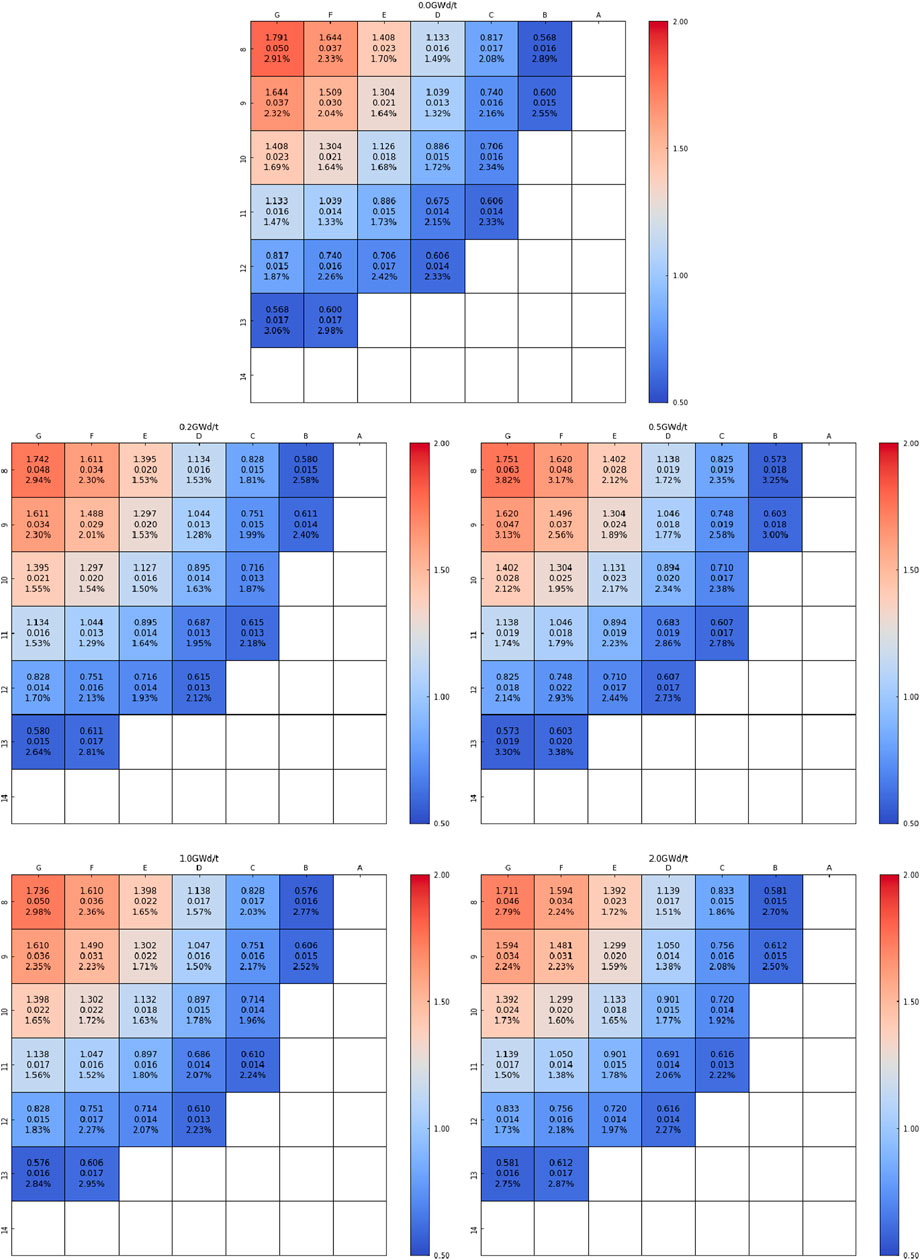
FIGURE 9. Power distribution prediction result of the BOC. First line: assembly average power. Second line: mean absolute error. Third line: average value of absolute relative error.

FIGURE 10. Power distribution prediction result of the MOC. First line: assembly average power. Second line: mean absolute error. Third line: average value of absolute relative error.
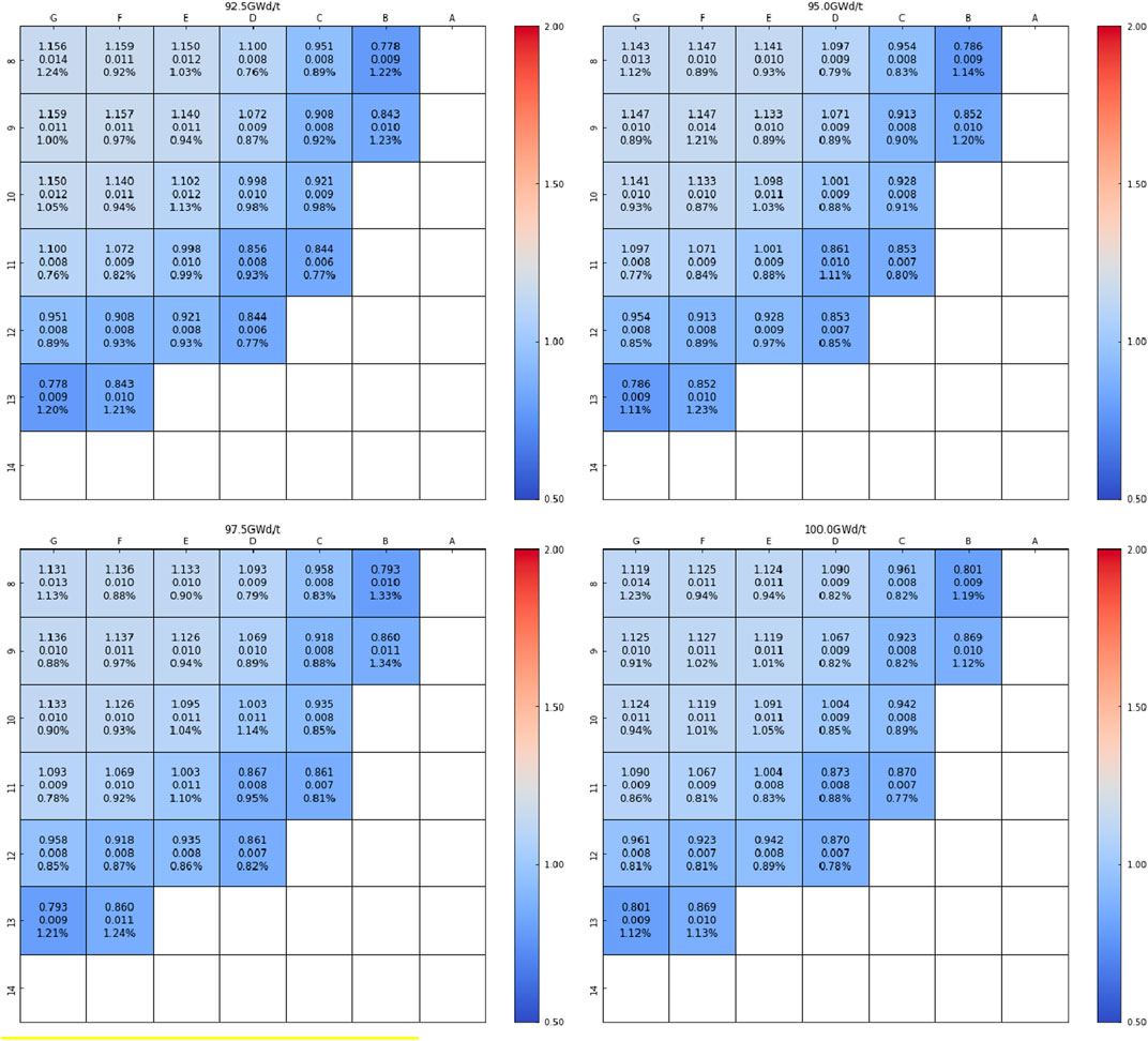
FIGURE 11. Power distribution prediction result of the EOC. First line: assembly average power. Second line: mean absolute error. Third line: average value of absolute relative error.
The average power of assembly decreases with the increase of the distance from the core center. The average absolute error shows the same trend. The error in the core center is higher than that in the core periphery. But the error is in the same level. For the average value of the absolute error, similar to eigenvalue prediction, the error in the BOC and MOC is higher than that in the EOC. In a specific burnup point, the error in the center region and peripheral region is higher than that in the inter-ring region. This phenomenon is caused by the spatial self-shielding effect. It means that there is different performance in different positions, even if the configuration is the same. Besides, the boundary condition, the reflector, and the void region exist in the core center and peripheral regions, which increases the difficulty of learning in these regions.
3.3 Discussion on Efficiency
In the process of evaluating the accuracy of models, the efficiency was also tested. During the diffusion calculation, each node was considered an assembly, and two-group constants were used. A steady-state diffusion calculation takes a few seconds, and the burnup calculation time can be neglected. It takes nearly 2 days to generate 1 million samples. However, for the neural network models obtained with training, it takes 18 s and 14 s to generate 0.2 million eigenvalues and PDs. The calculation efficiency is remarkably improved. For the CNN and FCN models, learning once (epoch) costs 23 s and 40 s, respectively. The detailed time comparison is listed in Table 4.
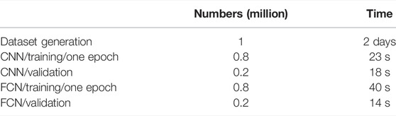
TABLE 4. Time comparison.
Similar to the application of neural network in other fields, the generalization of trained models is an issue. In the process of training, each assembly was labeled with a unique ID. The existing IDs cannot identify any new assembly. It directly leads to the lack of generalization ability. This is the limitation of neural networks in this study.
4 Conclusion
In this study, the CNN and the FCN were adopted to predict the eigenvalue and the power distribution for a simplified core during burnup, respectively. The loading pattern is encoded as a two-dimensional matrix as the models’ input. As a result of validating for 0.2 million samples, the performance of the trained models for the EOC is better than that for the BOC and MOC. For eigenvalue prediction, the fraction of the eigenvalue with error more than 500 pcm is less than 1% for all burnup points in the EOC. But there are third burnup points in the BOC and one burnup point in the MOC, where the fraction is over 1%. This is caused by the changes of reactivity balance between poison and fuel in the BOC and MOC. However, in the EOC, the differences between different assemblies become small as the poison nuclide depletes to a negligible level. With regard to the power distribution, the performance of the trained models for the EOC is better than that for the BOC and MOC, too. The mean absolute error of assembly power follows that the error decreases with the increasing distance from the core center. But the error is in the same level. The average value of absolute relative error in the center and peripheral regions is larger than that in the inter-ring region. It is caused by the self-shielding effect, which leads to the different performance in different positions, even if the configuration is the same. Besides, the presence of boundary condition and the fact that the same information is shared among different fuel positions also increase the difficulty of learning.
This investigation indicates that the neural network has the capability to predict core key parameters, such as the eigenvalue and power distribution. Compared with the conventional diffusion calculation, the introduction of neural network as the surrogate model significantly reduces the computation time. However, the error is influenced by the depletion and the assembly location. This indicates that it is not appropriate to directly use the ID of assembly as input in this research. The selection of the model input needs to be further analyzed.
Data Availability Statement
The original contributions presented in the study are included in the article/Supplementary Material, and further inquiries can be directed to the corresponding authors.
Author Contributions
JZ: Writing-original draft, Visualization, Simulation. YZ: Simulation. QZ (3rd author): Writing-review, Idea, Supervision. XW: Resources. QZ (5th author): Resources.
Funding
This work was supported by the National Natural Science Foundation of China (12105063), the Science and Technology on Reactor System Design Technology Laboratory (HT-KFKT-02-2019004), the Stability Support Fund for Key Laboratory of Nuclear Data (JCKY2021201C154), and the Natural Science Foundation of Heilongjiang Province of China (LH2020A001).
Conflict of Interest
The authors declare that the research was conducted in the absence of any commercial or financial relationships that could be construed as a potential conflict of interest.
Publisher’s Note
All claims expressed in this article are solely those of the authors and do not necessarily represent those of their affiliated organizations, or those of the publisher, the editors, and the reviewers. Any product that may be evaluated in this article, or claim that may be made by its manufacturer, is not guaranteed or endorsed by the publisher.
Supplementary Material
The Supplementary Material for this article can be found online at: https://www.frontiersin.org/articles/10.3389/fenrg.2022.851231/full#supplementary-material
References
Chollet, F. (2015). Keras. Available at: https://keras.io.
Hedayat, A., Davilu, H., and Sepanloo, K. (2009). Estimation of Research Reactor Core Parameters Using Cascade Feed Forward Artificial Neural Networks. Prog. Nucl. Energy 51 (6-7), 709–718. doi:10.1016/j.pnucene.2009.03.004
Jang, H. (2020). Application of Convolutional Neural Network to Fuel Loading Pattern Optimization by Simulated Annealing. Korea: Transactions of the Korean Nuclear Society Autumn Meeting.
Jang, H., and Lee, H. (2019). Prediction of Pressurized Water Reactor Core Design Parameters Using Artificial Neural Network for Loading Pattern Optimization. Korea: Transactions of the Korean Nuclear Society Spring Meeting.
Kim, H. G., Chang, S. H., and Lee, B. H. (1993a). Optimal Fuel Loading Pattern Design Using an Artificial Neural Network and a Fuzzy Rule-Based System. Nucl. Sci. Eng. 115 (2), 152. doi:10.13182/NSE93-A28525
Kim, H. G., Chang, S. H., and Lee, B. H. (1993b). Pressurized Water Reactor Core Parameter Prediction Using an Artificial Neural Network. Nucl. Sci. Eng. 113 (1), 70.
Krizhevsky, A., Sutskever, I., and Hinton, G. E. (2012). Imagenet Classification with Deep Convolutional Neural Networks. Adv. neural Inf. Process. Syst. 25, 1097.
Lee, G.-C., and Heung Chang, S. (2003). Radial Basis Function Networks Applied to DNBR Calculation in Digital Core Protection Systems. Ann. Nucl. Energy 30 (15), 1561–1572. doi:10.1016/s0306-4549(03)00099-9
Lee, J., Nam, Y., and Joo, H. (2019). Convolutional Neural Network for Power Distribution Prediction in PWRs. Jeju, Korea: Transactions of the Korean Nuclear Society Spring Meeting.
Leppänen, J., Pusa, M., and Valtavirta, V. (2015). The Serpent Monte Carlo Code: Status, Development and Applications in 2013. Ann. Nucl. Energy 82, 142. doi:10.1016/j.anucene.2014.08.024
Long, J., Shelhamer, E., and Darrell, T. (2015). “Fully Convolutional Networks for Semantic Segmentation,” in Proceedings of the IEEE conference on computer vision and pattern recognition, 3431–3440.
Mazrou, H., and Hamadouche, M. (2004). Application of Artificial Neural Network for Safety Core Parameters Prediction in LWRRS. Prog. Nucl. Energy 44 (3), 263–275. doi:10.1016/s0149-1970(04)90014-5
Niknafs, S., Ebrahimpour, R., and Amiri, S. (2010). Combined Neural Network for Power Peak Factor Estimation. Aust. J. Basic Appl. Sci. 4 (8), 3404.
Saber, A. S. (2015). “Nuclear Reactors Safety Core Parameters Prediction Using Artificial Neural Networks,” in 2015 11th International Computer Engineering Conference (ICENCO) (IEEE).
Souza, R. M. G., and Moreira, J. M. (2006). Neural Network Correlation for Power Peak Factor Estimation. Ann. Nucl. Energy 33 (7), 594. doi:10.1016/j.anucene.2006.02.007
Whyte, A., and Parks, G. (2020). “Surrogate Model Optimization of a ‘micro Core’ PWR Fuel Assembly Arrangement Using Deep Learning Models,” in Proc. Int. Conf. Physics of Reactors 2020 (PHYSOR 2020), Cambridge, United Kingdom.
Zhang, Q. (2019). “A Deep Learning Model for Solving the Eigenvalue of the Diffusion Problem of 2-D Reactor Core,” in Proceedings of the Reactor Physics Asia 2019 (RPHA19) Conference, Osaka, Japan, December 2–3, 2019.
Keywords: surrogate model, convolutional neural network, reactor design, eigenvalue prediction, power distribution prediction
Citation: Zhang J, Zhou Y, Zhang Q, Wang X and Zhao Q (2022) Surrogate Model of Predicting Eigenvalue and Power Distribution by Convolutional Neural Network. Front. Energy Res. 10:851231. doi: 10.3389/fenrg.2022.851231
Received: 09 January 2022; Accepted: 31 May 2022;
Published: 19 July 2022.
Edited by:
Jun Wang, University of Wisconsin-Madison, United StatesReviewed by:
Chunpeng Wu, Duke University, United StatesJiankai Yu, Massachusetts Institute of Technology, United States
Han Bao, Idaho National Laboratory (DOE), United States
Copyright © 2022 Zhang, Zhou, Zhang, Wang and Zhao. This is an open-access article distributed under the terms of the Creative Commons Attribution License (CC BY). The use, distribution or reproduction in other forums is permitted, provided the original author(s) and the copyright owner(s) are credited and that the original publication in this journal is cited, in accordance with accepted academic practice. No use, distribution or reproduction is permitted which does not comply with these terms.
*Correspondence: Jinchao Zhang, MTM5MzUzOTc5MTJAaHJiZXUuZWR1LmNu; Qian Zhang, emhhbmdxaWFuMDUxNUB6anUuZWR1LmNu