An Improved Model of the Heat Pipe Based on the Network Method Applied on a Heat Pipe Cooled Reactor

As the unique piece of heat transport equipment in a heat pipe cooled reactor, an accurate simulation of the heat pipe is helpful for understanding the real behavior of the reactor core and the reactor system. Based on the network method, an improved model for the heat pipe which considers the heat conductance in the wall, the vapor flow in the vapor space, and the liquid flow in the wick is proposed. Meanwhile, the gravity term is also added to the flow equation. Compared with the experimental results of a copper-water heat pipe, the validity of this model is verified. Then, a high-temperature sodium heat pipe of 1.0 m length is selected as the study object. Based on the analysis, it can be found that the total temperature difference of the heat pipe is 31.7 K, and the temperature drop caused by the vapor flow is only 2.6 K. As for the flow pressure drop in the heat pipe, the pressure drop is mainly concentrated in the wick region, which is 8,422.47 Pa, and the pressure drop in the vapor space is only 896.68 Pa. In cases of non-uniform heating and cooling, high heat leakage, and inclined operation, results indicate that the greater the non-uniformity of heating or cooling, the greater will be the temperature drop of the heat pipe. With the increase of heat leakage, the operating temperature of the heat pipe decreases significantly, and the total temperature drop increases. The heat pipe can operate at all positive inclination angles, but when the inclination angle exceeds$-{30}^{°}$, the heat pipe will reach the capillary limit, and it may be damaged. All of these results can provide support for the design and simulation of a heat pipe cooled reactor.

1 Introduction

Benefiting from the compact structure, low weight, and high reliability, a heat pipe cooled reactor can be widely used in aerospace, mobile power stations, deep-water exploration, and other fields. Many preliminary designs of heat pipe cooled reactor systems have been proposed, such as the Kilopower system (Poston et al., 2019), the Heatpipe-Operated Mars Exploration Reactor (HOMER) system (Poston, 2001), the (Heat Pipe-Segmented Thermoelectric Module Converter (HP-STMC) system (El-Genk and Tournier, 2004), the MegaPower reactor system (McClure et al., 2015), the eVinci reactor system (Swartz et al., 2021), and the Aurora reactor (Kadak, 2017). As the unique piece of equipment of fission heat absorption, the stable operation of the heat pipe is critical for the safety of the reactor system. Operating characteristics of the heat pipe can directly affect the power variation and temperature distribution of the reactor core. The accurate simulation of the heat pipe is important for reactor simulation and reactor design.

During the operation, the phenomena of heat conductance, heat convection, evaporation, and condensation exist in the heat pipe. Figure 1 shows the basic composition and the heat transport of the heat pipe. It is composed of a wall, wick, vapor space, and insulating layer. The wick consists of a porous structure and liquefied working medium. As for the porous structure, it can be wrapped screen, sintered metal, groove, open artery, or other types. Along the axial direction, it is divided into an evaporator, adiabatic section, and condenser. When it is heated, the working medium evaporates and generates vapor flows to the condenser with the effective pressure head. Then, the latent heat released by condensation transfers to the secondary by axial heat conduction and heat convection. With the pumping head of capillarity, the liquefied working medium flows back to the evaporator, thus completing the heat transfer circulation. Because of the temperature difference between the heat pipe and the environment, there will be a certain amount of heat lost to the environment through the insulating layer. Moreover, the heat transfer capacity of the heat pipe is always limited by heat transfer limitations such as the capillary limit, sonic limit, boiling limit, and entrainment limit (Busse, 1973), (Faghri, 1995), (Levy and Chou, 1973).

FIGURE 1

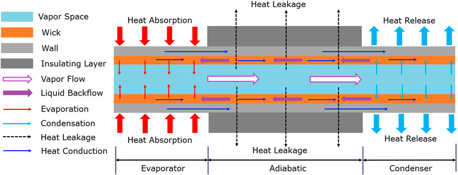
FIGURE 1. Basic diagram of the heat pipe structure and main heat transfer process.

So far, many theoretical analyses (Tournier and El-Genk, 1994; Tournier and El-Genk, 1996; Rice and Faghri, 2007) and experimental studies (El-Genk and Lianmin, 1993; Kim and Peterson, 1995; Xu and Zhang, 2005) have been carried out. In 1965, Cotter (1965) proposed the theory of the heat pipe for the first time, which laid the foundation for theoretical analyses of heat pipes. Cao and Faghri (1991) and (Cao and Faghri, 1993a) described vapor flow using two-dimensional Navier–Stokes (N–S) equations of compressible vapor and derived mass and energy transfer equations at the vapor–liquid interface. In the early startup period of high-temperature heat pipe operations, Cao and Faghri (1993b) adopted the self-diffusion model of rarefied vapor to describe vapor flow. The Knudsen number was chosen to judge the flow type of the vapor. However, this model still assumed that there was only heat conduction in the wick region. Heat transport caused by the backflow was also ignored. Faghri and Harley (1994) presented a transient lumped formulation for heat pipes. Because of the “isothermal” characteristics of the heat pipe, Faghri et al. treated the heat pipe as a control volume with uniform temperature distribution. Although this method greatly simplified modeling, only the lumped temperature was calculated which was insufficient to understand the operation characteristics of a heat pipe. Zuo and Faghri (1998) simplified the heat transportation of a heat pipe as heat conduction, ignoring the backflow in the wick and the temperature drop in the vapor space. The network model was established. Compared with the lumped model, it took the actual process of heat transportation into consideration and could obtain more information about the operation of the heat pipe. Therefore, it was widely used for the fast calculation of heat pipe performance. However, this model could not calculate the fluid flow and pressure drop during the operation. Ferrandi et al. (2013), inheriting the basic idea of the network model, regarded vapor flow as an adiabatic flow of compressible fluid to preliminarily analyze the vapor flow. However, in this model, the heat transfer between the vapor space and the wick in the adiabatic region and fluid backflow were both ignored, leading to the incapability of calculating the real temperature distribution of the heat pipe.

In recent years, many researchers have used the computational fluid dynamics (CFD) method to simulate the heat transport characteristics of heat pipes. Alizadehdakhel et al. (2010) had investigated the effect of input heat flow and fill ratio on the performance of the thermosiphon. They showed that the CFD method was useful for calculating the complex flow and heat transfer in the thermosiphon. Annamalai and Ramalingam (2011) had analyzed the characteristics of heat pipes using ANSYS CFX. They concluded that for efficient operation of the heat pipe; the condenser surface should be exposed to circulating water with a high convective coefficient, or a higher heat transfer area is required with the addition of fins in the condenser section. Lin et al. (2013) had studied the heat transfer mechanism of a miniature oscillating heat pipe (MOHP) using ANSYS FLUENT. The volume of the fluid (VOF) model and a mixture model were used for comparison. Results showed that the mixture model was more suitable for the two-phase flow simulation in an MOHP. Boothaisong et al. (2015) had established a three-dimensional model to simulate the heat transfer on heat pipes. The governing equation based on the shape of the pipe was numerically simulated using the finite element method. Yue et al. (2018) had executed the CFD simulation on the heat transfer and flow characteristics of micro-channel separate heat pipes under different filling ratios. The CFD method can realize the three-dimensional modeling of heat pipes. Important phenomena of the two-phase flow, evaporation, condensation, and entrainment can also be simulated. However, it consumes a lot of computing resources and calculates slowly. Moreover, for different sizes and types of heat pipes, geometry establishment and mesh generation have to be carried out which means that the flexibility of the model is poor.

For heat pipe cooled reactor systems, situations of non-uniform heating and cooling, heat leakage, and inclined operation may occur. The existing models either cannot consider these factors comprehensively or have shortcomings of a low calculation efficiency. In this study, an improved model based on the network method is proposed. It realizes the fast and flexible calculation of the heat pipe performance, and it can obtain the variation of temperature, flow rate, pressure drop, and other parameters. After verifying the validity of the model by comparing with the experimental results of the copper-water heat pipe, the operating characteristics of high-temperature sodium heat pipes are analyzed in different cases. The effects of a non-uniform heat transfer, heat leakage, and gravity on heat pipe operations are discussed in detail.

2 Description of the Improved Network Model

First, both the method and main limitations of a network model are described in Section 2.1. In Section 2.2, the improved model is demonstrated, and the conservation equations of each region are established. According to the modification of this model, it can calculate the temperature distribution of the heat pipe and can obtain the flow characteristics and pressure distribution.

2.1 Network Model for Heat Pipes

Zuo and Faghri (1998) had proposed the classical network model for heat pipes in 1996 (Figure 2), which had been widely used in heat pipe cooled reactor simulation (Yuan et al., 2016). For this model, it was considered that the heat absorbed in the evaporator was transported to the condenser through heat conductance, and the temperature drop caused by the vapor flow was ignored. Meanwhile, it ignored the high-speed vapor flow in the vapor space, the fluid backflow in the wick, and the evaporation/condensation at the vapor–liquid interface. Since only six temperature variables need to be calculated, it can obtain the fast calculation of heat pipe performance. But the information on fluid flow and pressure distribution is lost.

FIGURE 2

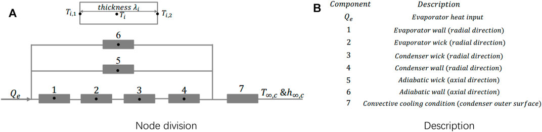
FIGURE 2. Traditional network model for a heat pipe.

2.2 Improved Network Model for Heat Pipe

Figure 3 shows the node division for this improved model. To account for the non-uniform heat transfer and heat leakage, several temperature nodes are set in each region. The actual number of nodes can be flexibly adjusted based on the actual length of each region and the requirement of computational accuracy. Both the axial and the radial heat conductance are included at each node. Particularly, the heat transportation of the liquid backflow in the wick and evaporation or condensation between the wick and the vapor space are contained to realize the simulation of heat pipe operations as real as possible. Meanwhile, the gravity term is added to the flow equations to preliminarily analyze the operating characteristics under different angles of inclination. Particularly, if the fluid flow, evaporation, condensation, and heat leakage were all ignored, this model would degenerate into the network model. It should be mentioned that this model cannot be used for the transient calculation on heat pipe startups because the melting and redistribution of the working medium are not included in this model.

FIGURE 3

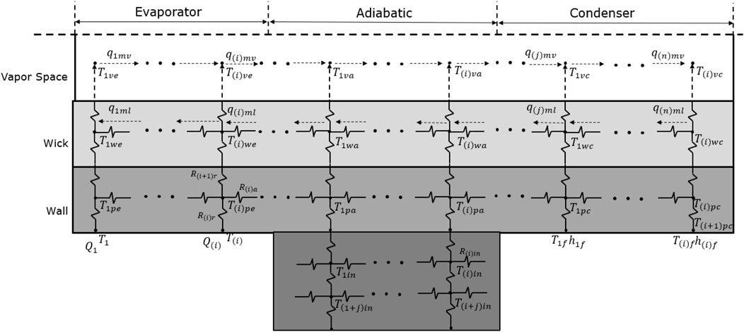
FIGURE 3. Schematic diagram of the improved heat pipe model.

To simplify the modeling difficulty, there are some assumptions:

1) Heat conduction is two-dimensional;

2) Vapor flow is a one-dimensional, compressible, and adiabatic flow;

3) Vapor is treated as a compressible ideal gas;

4) Liquid in the wick is incompressible, and the wick volume is constant;

5) Gravity does not cause the redistribution of the working medium;

6) The temperature at the vapor–liquid interface is always the saturated temperature.

Actually, when the working medium is completely melted, there will be an accumulation of the working medium caused by gravity. The redistribution of the working medium may affect the operation of the heat pipe. Further studies will be executed to discuss the effect of gravity.

In this model, there are radial thermal resistance, axial thermal resistance, and convective thermal resistance. They are defined as follows:

$\text{Radial}\text{thermal}\text{resistance:}{R}_{\left(i\right)r}=\frac{\text{ln}\left(r_{out}/r_{in}\right)}{2\pi k_{\left(i\right)}{L}_{\left(i\right)}},(1)$

$\text{Axial}\text{thermal}\text{resistance:}{R}_{\left(i\right)a}=\frac{L_{\left(j\right)}}{\pi \left(r_{out}^2-r_{in}^2\right)k_{\left(i\right)}},(2)$

$\text{Convective}\text{thermal}\text{resistance:}{R}_{\left(i\right)f}=\frac{1}{2\pi r_{out}{L}_{\left(k\right)}{\lambda }_{\left(i\right)}}.(3)$

2.2.1 Modeling in the Wall Region

Along the axial direction, the wall is divided into three regions. The Neumann boundary condition is set on the boundary surface of the evaporator. There can be different heating powers for each node. The conservation equation can be written as follows:

${\rho }_{\left(i\right)pe}{C}_{\left(i\right)pe}\frac{d{T}_{\left(i\right)pe}}{dt}=Q_{\left(i\right)in}+\frac{T_{\left(i-1\right)pe}-T_{\left(i\right)pe}}{R_{\left(i-1\right)a}}-\frac{T_{\left(i\right)pe}-T_{\left(i+1\right)pe}}{R_{\left(i\right)a}}-\frac{T_{\left(i\right)pe}-T_{\left(i\right)we}}{R_{\left(i+1\right)r}+R_{\left(i+2\right)r}}.(4)$

As for the wall region in the adiabatic section, there is heat conduction between the wall and the insulating layer. Thermal contact resistance between two regions is ignored.

${\rho }_{\left(i\right)pa}{C}_{\left(i\right)pa}\frac{d{T}_{\left(i\right)pa}}{dt}=\frac{T_{\left(i-1\right)pa}-T_{\left(i\right)pa}}{R_{\left(i-1\right)a}}+\frac{T_{\left(i\right)wa}-T_{\left(i\right)pa}}{R_{\left(i+1\right)r}+R_{\left(i+2\right)r}}-\frac{T_{\left(i\right)pa}-T_{\left(i+1\right)pa}}{R_{\left(i\right)a}}-\frac{T_{\left(i\right)pa}-T_{\left(i\right)in}}{R_{\left(i\right)r}+R_{\left(i\right)in}}.(5)$

Actually, if it is needed to consider the contact conductance, adding the thermal contact resistance on the radial heat transfer path between two regions is feasible (Figure 4). The thermal contact resistance can be obtained through empirical relations or contact heat transfer models (Song and Yovanovich, 1988) (Kumar and Ramamurthi, 2001).

$Q_{radial}=\frac{T_{pa}-T_{in}}{R_{pr}+R_{in}+R_{gap}}.(6)$

FIGURE 4

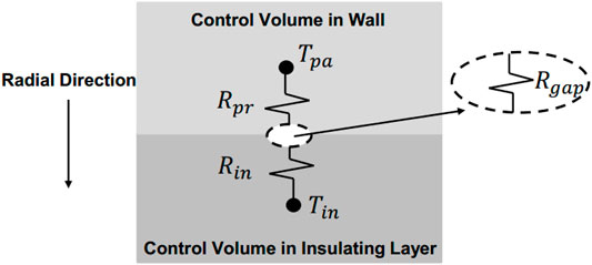
FIGURE 4. Contact heat transfer between the wall and insulating layer.

On the condenser wall surface, the Robin boundary condition is adopted as follows:

${\rho }_{\left(i\right)pc}{C}_{\left(i\right)pc}\frac{d{T}_{\left(i\right)pc}}{dt}=\frac{T_{\left(i-1\right)pc}-T_{\left(i\right)pc}}{R_{\left(i-1\right)a}}+\frac{T_{\left(i\right)wc}-T_{\left(i\right)pc}}{R_{\left(i+1\right)r}+R_{\left(i+2\right)r}}-\frac{T_{\left(i\right)pc}-T_{\left(i+1\right)pc}}{R_{\left(i\right)a}}-\frac{T_{\left(i\right)pc}-T_{\left(i\right)f}}{R_{\left(i\right)r}+R_{\left(i\right)f}}.(7)$

For the surface temperature of the wall, the continuous heat flow criterion is used for deducing the temperature:

$Q_{\left(i\right)in}=A_{\left(i\right)pe}{k}_{\left(i\right)pe}\frac{T_{\left(i\right)}-T_{\left(i\right)pe}}{Thic{k}_{\left(i\right)}},(8)$

$\frac{T_{\left(i\right)pc}-T_{\left(i\right)f}}{R_{\left(i\right)r}+R_{\left(i\right)f}}=\frac{T_{\left(i\right)pc}-T_{\left(i+1\right)pc}}{R_{\left(i\right)r}}.(9)$

Thus, the surface temperature can be obtained as follows:

$T_{\left(i\right)}=T_{\left(i\right)pe}+\frac{Q_{\left(i\right)in}}{A_{\left(i\right)pe}{k}_{\left(i\right)pe}}Thic{k}_{\left(i\right)},(10)$

$T_{\left(i+1\right)pc}=T_{\left(i\right)pc}-\frac{T_{\left(i\right)pc}-T_{\left(i\right)f}}{R_{\left(i\right)r}+R_{\left(i\right)f}}{R}_{\left(i\right)r}.(11)$

2.2.2 Modeling in the Insulating Layer

Similarly, the temperature nodes in this region can be increased or decreased based on the calculation requirement. Conservation equations can be obtained as follows:

${\rho }_{\left(i\right)in}{C}_{\left(i\right)in}\frac{d{T}_{\left(i\right)in}}{dt}=\frac{T_{\left(i-1\right)in}-T_{\left(i\right)in}}{R_{\left(i-1\right)in}}+\frac{T_{\left(i\right)pa}-T_{\left(i\right)in}}{R_{\left(i+1\right)r}+R_{\left(i+2\right)r}}-\frac{T_{\left(i\right)in}-T_{\left(i+1\right)in}}{R_{\left(i\right)in}}-\frac{T_{\left(i\right)in}-T_{\left(i+j\right)in}}{R_{\left(i\right)r}}.(12)$

2.2.3 Modeling in the Wick Region

2.2.3.1 Temperature Equations

Heat transfer in the wick is shown in Figure 5. It includes evaporation/condensation, radial heat conduction, axial heat conduction, and heat transport of the working medium backflow. Evaporation/condensation between the vapor space and the wick can be expressed, as shown in Figure 6. According to the assumptions (2) and (6), the vapor temperature is considered to be equal to the vapor–liquid interface temperature.

$T_v=T_f,(13)$

$Q_{evap/cond}=\frac{T_i-T_f}{R_i}=\frac{T_i-T_v}{R_i}.(14)$

FIGURE 5

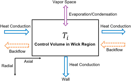
FIGURE 5. Heat transfer process in the wick.

FIGURE 6

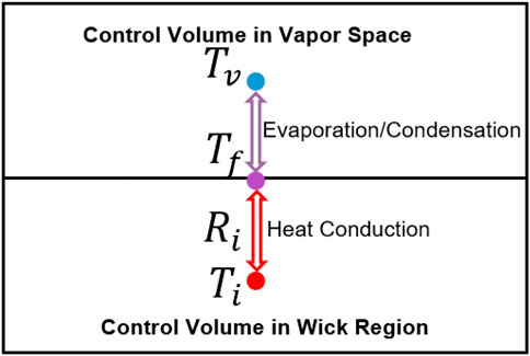
FIGURE 6. Evaporation/condensation between the wick and the vapor space.

Heat transfer by evaporation/condensation can be obtained as follows:

$\text{Evaporator:}{Q}_{evap}=\frac{T_{\left(i\right)we}-T_{\left(i\right)ve}}{R_{\left(i+1\right)r}},(15)$

$\text{Adiabatic}\text{section:}{Q}_{adia}=\frac{T_{\left(i\right)va}-T_{\left(i\right)wa}}{R_{\left(i+1\right)r}},(16)$

$\text{Condenser:}{Q}_{cond}=\frac{T_{\left(i\right)vc}-T_{\left(i\right)wc}}{R_{\left(i+1\right)r}}.(17)$

The mass flow rate can also be obtained as follows:

$\text{Evaporator:}{q}_{evap}=\frac{T_{\left(i\right)we}-T_{\left(i\right)ve}}{R_{\left(i+1\right)r}{h}_v\left(T_{\left(i\right)ve}\right)},(18)$

$\text{Adiabatic}\text{section:}{q}_{adia}=\frac{T_{\left(i\right)va}-T_{\left(i\right)wa}}{R_{\left(i+1\right)r}{h}_v\left(T_{\left(i\right)va}\right)},(19)$

$\text{Condenser:}{q}_{cond}=\frac{T_{\left(i\right)vc}-T_{\left(i\right)wc}}{R_{\left(i+1\right)r}{h}_v\left(T_{\left(i\right)vc}\right)}.(20)$

According to the assumption (4), the backflow rate in the wick core can be obtained as follows:

$q_{\left(i\right)ml}={\displaystyle \sum _{j=i+1}^{12}{q}_{\left(j\right)v}},\{\begin{array}{cc}{q}_{\left(j\right)v}<0& evaporation,\\ q_{\left(j\right)v}>0& condensation.\end{array}(21)$

Therefore, the energy equation can be summarized as follows:

${\rho }_{\left(i\right)we}{C}_{\left(i\right)we}\frac{d{T}_{\left(i\right)we}}{dt}=\frac{T_{\left(i-1\right)we}-T_{\left(i\right)we}}{R_{\left(i-1\right)a}}-\frac{T_{\left(i\right)we}-T_{\left(i+1\right)we}}{R_{\left(i\right)a}}-\frac{T_{\left(i\right)we}-T_{\left(i\right)ve}}{R_{\left(i+1\right)r}}-\frac{T_{\left(i\right)we}-T_{\left(i\right)pe}}{R_{\left(i\right)r}+R_{\left(i-1\right)r}}+q_{\left(i\right)ml}{h}_{\left(i\right)l} -q_{\left(i-1\right)ml}{h}_{\left(i-1\right)l}.(22)$

2.2.3.2 Flow Equations

The wick is regarded as a porous structure. The porous medium model is used for describing the flow of the working medium. In addition, the gravity term is added in the equation as follows:

$\text{ρg}+\nabla P=-\frac{\mu }{K}u.(23)$

Definition of the liquid flow rate is

$q_{ml}={\rho }_f\epsilon \pi \left(r_{out}^2-r_{in}^2\right)u.(24)$

Combining Eq. 23 with Eq. 24 and integrating on length $L_{eff}$ we obtain the following equation:

$\frac{\mu L_{eff}}{K{\rho }_f}\frac{1}{\epsilon \pi \left(r_{out}^2-r_{in}^2\right)}{q}_{ml}=P_1-P_2+{\rho }_{f}g{L}_{eff}\mathrm{sin\theta }\mathrm{.}(25)$

In other words,

$P_2-P_1=\nabla P=\frac{\mu L_{eff}}{K{\rho }_f}\frac{1}{\epsilon \pi \left(r_{out}^2-r_{in}^2\right)}{q}_{ml}-{\rho }_{f}g{L}_{eff}\mathrm{sin\theta }\mathrm{.}(26)$

The permeability parameter $K$ can be estimated using the following empirical correlation.

$K=\frac{4r_g^2{\epsilon }^2}{150{\left(1-\epsilon \right)}^2}.(27)$

Therefore, the pressure drop caused by the flow in the wick can be solved when the flow rate is known.

2.2.3.3 Physical Parameter Calculation in the Wick

The wick is composed of a porous structure and liquefied working medium. In this model, two different materials are regarded as the equivalent material. The physical parameters such as density, specific heat capacity, and thermal conductivity coefficient can be calculated by the following formula (Bowman, 1991):

${\rho }_{equ}=\epsilon {\rho }_f+\left(1-\epsilon \right){\rho }_w,(28)$

$C_{equ}=\epsilon C_f+\left(1-\epsilon \right)C_w,(29)$

$k_{equ}=k_l\frac{\left(k_l+k_w\right)-\left(1-\epsilon \right)\left(k_l-k_w\right)}{\left(k_l+k_w\right)+\left(1-\epsilon \right)\left(k_l-k_w\right)}.(30)$

2.2.4 Modeling in the Vapor Space

2.2.4.1 Vapor Density Equations

In the vapor space, there are evaporation, condensation, and vapor flow. Using the law of conservation of mass, the vapor density equation can be obtained as follows:

$V_{\left(i\right)v}\frac{d{\rho }_{\left(i\right)v}}{dt}=q_{\left(i\right)v}+q_{\left(i-1\right)mv}-q_{\left(i\right)mv}.(31)$

2.2.4.2 Vapor Pressure Equations

Based on the assumption (2), the relation between pressure and density can be obtained by the following equation:

$\frac{\partial P_v}{\partial {\rho }_v}=\gamma R_g{T}_v.(32)$

So

$\frac{d{\rho }_v}{dt}=\frac{1}{\gamma R_g{T}_v}\frac{d{p}_v}{dt}.(33)$

Taking this correlation into Eq. 31, the vapor pressure equation can be obtained:

$\frac{d{P}_{\left(i\right)v}}{dt}=\frac{\gamma R_g{T}_{\left(i\right)v}}{V_{\left(i\right)v}}\left(q_{\left(i\right)v}+q_{\left(i-1\right)mv}-q_{\left(i\right)mv}\right).(34)$

2.2.4.3 Vapor Temperature Equations

Similarly, according to the assumptions, the relationship between the pressure and temperature can be obtained:

$\frac{\gamma }{\gamma -1}\frac{P_v}{T_v}\frac{d{T}_v}{dt}=\frac{d{P}_v}{dt}.(35)$

Combined with Eq. 34, the vapor temperature equation can be written as follows:

$\frac{d{T}_{\left(i\right)v}}{dt}=\frac{\left(\gamma -1\right)R_g}{V_{\left(i\right)v}}\frac{T_{\left(i\right)v}^2}{P_{\left(i\right)v}}\left(q_{\left(i\right)v}+q_{\left(i-1\right)mv}-q_{\left(i\right)mv}\right).(36)$

2.2.4.4 Vapor Flow Equations

For the vapor flow in the vapor space, it is assumed to be a one-dimensional, unsteady, and compressible laminar flow. In the N–S equation, it contains the time term, gravity axial term, convective transport term, surface friction term, and pressure gradient term. It can be seen as follows (Bowman, 1991):

$\frac{\partial \left(\rho u\right)}{\partial t}=\rho gsin\theta -\frac{\partial \left(\rho u^2\right)}{\partial x}-\frac{2{\tau }_w}{R}-\frac{\partial P}{\partial x}.(37)$

Integrating this equation on length $L_v$, it can be concluded as follows:

$\frac{L_v}{\pi r_i^2}\frac{d{q}_v}{dt}={\rho }_{v}g{L}_v\mathrm{sin\theta }+{\left(\frac{q_v^2}{{\rho }_v{\pi }^2{r}_i^4}\right)}_{1v}-{\left(\frac{q_v^2}{{\rho }_v{\pi }^2{r}_i^4}\right)}_{2v}-\frac{8\mu L_v}{{\rho }_v\pi r_i^4}{q}_v+P_{1v}-P_{2v}.(38)$

Appling Eq. 38 into the calculation of the working medium flow in the vapor space, we obtain the following equation:

$\frac{L_{\left(i\right)v}}{\pi r_{in}^2}\frac{d{q}_{\left(i\right)mv}}{dt}=-\frac{8\mu L_{\left(i\right)v}}{{\rho }_{\left(i\right)v}\pi r_{in}^4}{q}_{\left(i\right)mv}+\frac{1}{{\rho }_{\left(i\right)v}{\pi }^2{r}_{in}^4}{q}_{\left(i\right)in}^2-\frac{1}{{\rho }_{\left(i+1\right)v}{\pi }^2{r}_{in}^4}{q}_{\left(i\right)out}^2+P_{\left(i\right)v}-P_{\left(i+1\right)v}+{\rho }_{\left(i\right)v}g{L}_{\left(i\right)v}\mathrm{sin\theta }\mathrm{.}(39)$

2.3 Judgment of the Capillary Limit

At the vapor–liquid interface between the wick and vapor space, the concave vapor–liquid surface can form the pumping head of the capillarity (Figure 7). The pumping head acts as the power of the stable flow. When the heat absorption of the evaporator exceeds a certain limitation, the liquid returned by the pumping head cannot meet the required flow rate of evaporation, and the temperature in the evaporator will rise rapidly as a consequence of drying up in the wick. The heat pipe may be damaged.

FIGURE 7

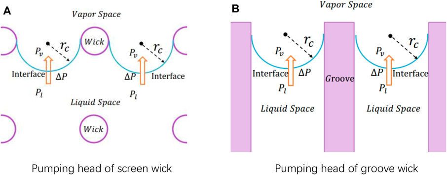
FIGURE 7. Pumping head of the capillarity.

The maximum pumping head of the capillarity provided by the heat pipe is as follows:

$P_v-P_l=\frac{2\sigma }{r_c}.(40)$

To ensure that the heat pipe is always below the capillary limit, the following relation needs to be met:

$\frac{2\sigma }{r_c}\ge {\displaystyle \sum _{i=1}^{11}{P}_{\left(i\right)v}}+{\displaystyle \sum _{j=1}^{11}{P}_{\left(j\right)l}}+{\displaystyle \underset{0}{\overset{L}{\int }}{\rho }_{l}g\mathrm{sin\theta }dl}-{\displaystyle \underset{0}{\overset{L}{\int }}{\rho }_{v}gsin\theta dl}.(41)$

According to Eqs. 26,34, the pressure drop on each flow path can be calculated. When the angle of inclination is known, Eq. 41 can be adopted to judge whether the heat pipe reaches the capillary limit.

2.4 Numerical Algorithm of the Improved Model

The presented heat pipe model can be expressed as follows:

$\{\begin{array}{c}\frac{d\mathit{Y}}{dt}=f\left(t,\mathit{Y}\right)\\ Y\left(t_0\right)={\mathit{Y}}_0\end{array}.(42)$

Unknown variables including the temperature, density, pressure, and flow rate can be calculated as follows:

$\mathit{Y}=\left[T_{\left(i\right)pe},T_{\left(i\right)pa},T_{\left(i\right)pc,}{T}_{\left(i\right)we},T_{\left(i\right)wa},T_{\left(i\right)wc},T_{\left(i\right)ve},T_{\left(i\right)va},T_{\left(i\right)vc,}{\rho }_{\left(i\right)ve},{\rho }_{\left(i\right)va},{\rho }_{\left(i\right)vc,}{P}_{\left(i\right)ve},P_{\left(i\right)va},P_{\left(i\right)vc,}{q}_{\left(j\right)mv},T_{\left(k\right)in}\right].(43)$

Methods for solving this type of differential equation can be the Euler algorithm, Runge–Kutta algorithm, linear multistep method, and so on. In this study, the implicit Runge–Kutta algorithm is used. The basic solving process of this algorithm is as follows:

$\{\begin{array}{c}{\mathit{Y}}_{n+1}={\mathit{Y}}_n+h{\displaystyle \sum _{i=1}^m{b}_i{k}_i}\\ k_{i,j}=f\left(t_n+{\tau }_{i}h,{\mathit{Y}}_n+h{\displaystyle \sum _{j=1}^m{a}_{ij}{k}_j}\right)i=\mathrm{1,2},\cdots m\end{array}.(44)$

here, $t_n=t_0+nh\left(n=\mathrm{0,1},\cdots \right)$, $h$ is the transient time step, $b=\left[b_1,b_2,\cdots b_m\right]$ is the weight coefficient vector, $\tau =\left[{\tau }_1,{\tau }_2,\cdots {\tau }_m\right]$ is the node coefficient vector, and $a=\left[a_{11},a_{12},\cdots a_{1m},a_{21},a_{22},\cdots a_{2m},\cdots a_{mm}\right]$ is the coefficient matrix.

3 Model Validation

To verify the correctness of this model, experimental results of a copper-water heat pipe (Tournier and El-Genk, 1994) (Huang et al., 1993) are chosen. The description of this heat pipe is shown in Table.1.

TABLE 1

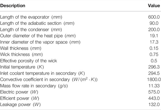
TABLE 1. Basic description of a copper-water heat pipe (Huang et al., 1993).

In calculation, the effective power is regarded as the real power in the evaporator. It is assumed that the heat pipe system is well insulated, and there is no heat leakage. For the evaporator, heat source distribution is assumed to be uniform. For the condenser, the convective coefficient is constant, and the fluid temperature at the corresponding node is calculated according to the law of conservation of energy.

$\begin{array}{cc}{T}_{\left(i\right)f}={\displaystyle \sum _{j=1}^{i-1}\left(\frac{T_{\left(j\right)pc}-T_{\left(j\right)f}}{R_{\left(j\right)pc}+R_{\left(j\right)f}}\right)/C_f+T_{1f}}& i=\mathrm{1,2,3,4}\end{array}.(45)$

The model predictions are compared with the experimental results of Huang et al. (1993) and the calculated results using the proposed heat pipe transient analysis model (HPTAM) of Tournier and El-Genk (1994) for horizontal water heat pipes (Figure 8). Based on the experimental data, the variation of effective power in the evaporator is fitted linearly, and the fitting formula is used for describing the real change of the heating power in the model (Figure 9).

FIGURE 8

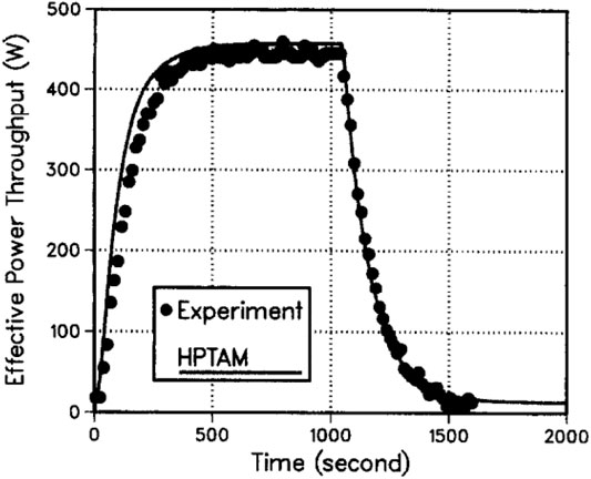
FIGURE 8. Original data of effective power (Tournier and El-Genk, 1994).

FIGURE 9

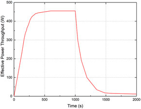
FIGURE 9. Fitted curve of effective power.

In this model, each region contains multiple temperature nodes. The arithmetic mean value of the temperature nodes in the corresponding region is selected for the comparison between these results. Figure 10 shows the temperature variation of the heat pipe with time. The curve shows the calculated results using this model, and the scatter is the measuring results by experiment. From the figure, it can be found that the calculated results are in good agreement with the experimental results. Meanwhile, it can be seen that there is little difference between the vapor temperature in the evaporator and that in the condenser. For the water heat pipe, the temperature drop in the vapor space can indeed be ignored. Figures 11, 12 show the temperature distribution in a steady state. Benefiting from the capability of describing non-uniform cooling, this model can calculate the temperature rise on the wall surface of the condenser section, causing the rise of the wall temperature. As a consequence, the correctness of this model is validated.

FIGURE 10

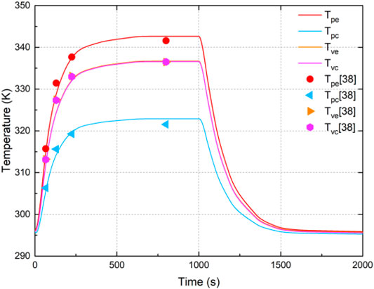
FIGURE 10. Comparison with experimental results.

FIGURE 11

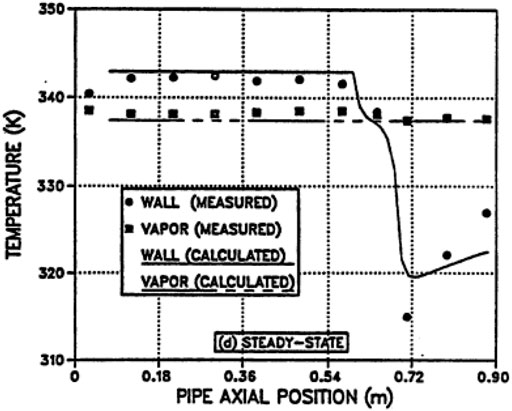
FIGURE 11. Temperature distribution in the steady state (Tournier and El-Genk, 1994).

FIGURE 12

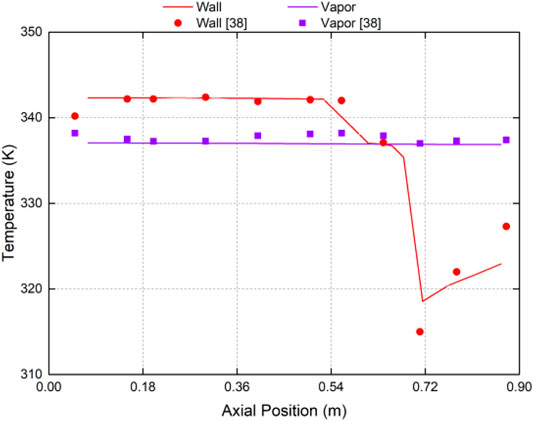
FIGURE 12. Calculated temperature distribution in the steady state.

4 Case Analysis

Four cases of standard operation, non-uniform heat transfer, heat leakage, and inclined operation are respectively carried out to analyze the operating characteristics of the heat pipe. They are also the situations that may occur during the operation of the heat pipe cooled reactor. A hypothetical high-temperature sodium heat pipe is taken as the research object. The basic description of this heat pipe is listed in Table 2. As for the physical parameters of sodium, such as density, heat capacity, thermal conductivity, enthalpy, and surface tension, they can be found in the report published by the Argonne National Laboratory (Fink and Leibowitz, 1995).

TABLE 2

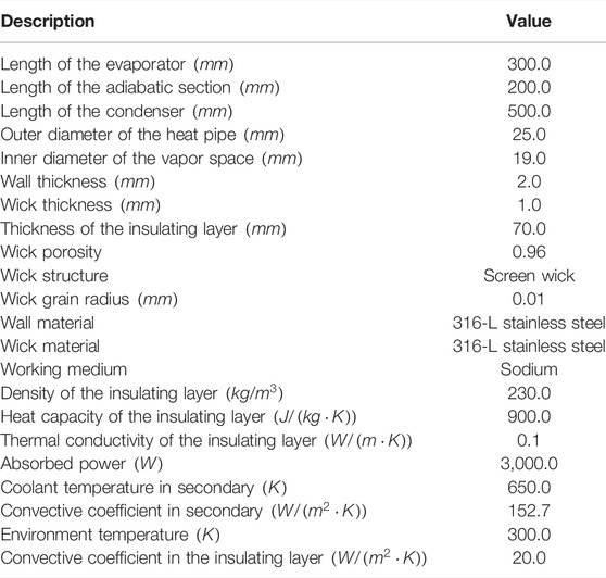
TABLE 2. Parameter description of a sodium heat pipe.

4.1 Case With Standard Operation

In this case, it is assumed that the heat pipe is uniformly heated and uniformly cooled. The insulating layer is treated as natural convection with the environment. Figure 13 shows the temperature distribution along the heat transport path. The arithmetic mean value of the corresponding region is chosen as the characteristic temperature. The surface temperature of the wall is calculated by Eqs. 10, 11 and considers this influence on the temperature distribution of the heat pipe. From Figure 13, it can be seen that the total temperature drop of this heat pipe is 31.7 K. The temperature drop in the evaporator is more obvious than that in the condenser. It is because the shorter length of the evaporator causes higher radial thermal resistance, and the higher thermal resistance leads to a larger temperature drop.

FIGURE 13

FIGURE 13. Temperature distribution along heat transport path.

As shown in Figure 14, the temperature distribution in each region is generally uniform, and the temperature drop in the axial direction is mainly concentrated in the transition section between different regions. The wall temperature difference between the evaporator and the adiabatic section is 13.8 K, and the temperature difference between the adiabatic section and the condenser is 8.1 K. As for the surface temperature differences, they are 19.1 and 13.6 K.

FIGURE 14

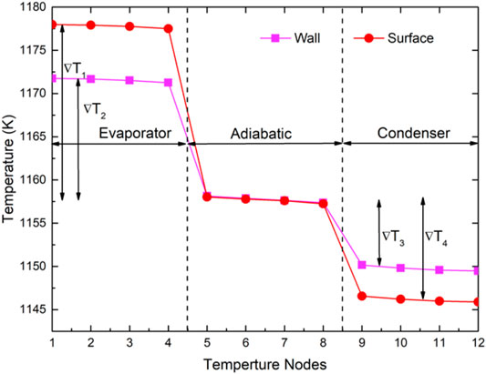
FIGURE 14. Temperature distribution along the heat transport path.

Figure 15 shows the temperature distribution of the wick and the vapor space along the axial direction. The broken line represents the wick temperature distribution using the network model. In that model, the evaporation, condensation, and working medium backflow are all ignored, which means only axial heat conduction exists in the wick. Therefore, the calculated temperature distribution of the wick is linear. From Figure 15, it can be found that the results of the improved model are more reasonable. In the evaporator and condenser, there is always a temperature difference between the wick and vapor space due to the evaporation and condensation of the liquid medium. The wick temperature in the adiabatic section remains basically the same as that of the vapor space, with only a temperature difference of about 0.04 k. The reason is shown in Figure 5. Heat transfer modes in the wick include axial heat conduction, radial heat conduction, evaporation/condensation heat transfer, and heat transport of fluid backflow. In this case, the axial heat conduction is not obvious. The radial heat conduction due to heat leakage and the working medium backflow causes a heat loss of the control volume. The heat release of condensation between the vapor space and wick can compensate for such heat loss to keep the temperature constant. Because the heat loss is not obvious, the condensing flow is small, causing only a small temperature difference between the wick and the vapor space. In addition, it can be found that the temperature difference in the vapor space is about 2.6 K due to the energy dissipation caused by high-speed flow and wall friction.

FIGURE 15

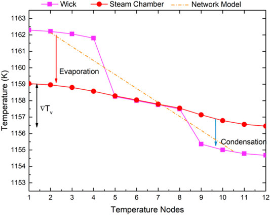
FIGURE 15. Temperature distribution of the wall and the surface in the axial direction.

This model can also simulate the flow distribution and pressure variation during the flow circulation. In this case, it is assumed that the heat pipe is uniformly heated, and the vapor flow rate increases linearly along the axial direction (Figure 16). Because of the good insulation of the adiabatic section, the condensation in this area is negligible. When the vapor flows to the condenser, the flow rate decreases sharply because of the condensation. Figure 17 shows the pressure variation in flow circulation. Although the vapor density is lower, there is still a pressure drop of about 897.2 Pa in the vapor chamber due to the accelerated pressure drop and frictional pressure drop of the vapor flow. In the wick region, caused by the viscous flow in the porous medium, the pressure drop is about 6,159.1 Pa. Then, with the pumping head of capillarity, the pressure rises to maintain the stable flow.

FIGURE 16

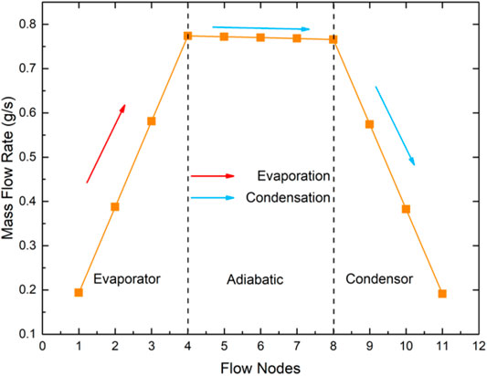
FIGURE 16. Temperature distribution of the wick and the vapor space.

FIGURE 17

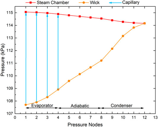
FIGURE 17. Mass flow rate in the vapor space.

4.2 Case With Non-Uniform Heating and Cooling

In a heat pipe cooled reactor, heating and cooling to a high-temperature heat pipe are always non-uniform. In this section, these effects on a heat pipe are preliminarily discussed. The steady-state performance of heat pipes under different boundary conditions is discussed. A detailed description of different cases is shown in Table 3.

TABLE 3

TABLE 3. Description of a non-uniform heat transfer boundary condition.

Figure 18 shows the temperature distribution of the wall in different cases. From the figure, it can be seen that the non-uniform boundary condition does change the temperature distribution in the corresponding regions. The actual temperature distribution is determined by the specific boundary condition. In general, the higher the heating power, the higher will be the temperature. The more the cooling power, the lower temperature will be. Meanwhile, it can be found that non-uniform heating and non-uniform cooling both lead to a larger temperature difference in the heat pipe. The greater the non-uniformity is, the larger the temperature difference will be. In case 5, the total temperature difference is 33.76 K, which is up to 19.54% compared with the standard case.

FIGURE 18

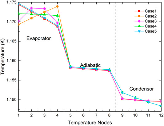
FIGURE 18. Pressure variation in circulation.

Combining Figures 18, 19, it can be concluded that non-uniform heating does not affect the temperature distribution of the condenser and non-uniform cooling does not change the temperature distribution of the evaporator. It is because the non-uniformity of heating or cooling does not obviously change the vapor temperature in the vapor space. For the heat transport between the evaporator and condenser, it is achieved through flow heat transfer of the vapor. The high-speed flow of the vapor can effectively eliminate the influence of non-uniform heat transfer on the operation of the heat pipe.

FIGURE 19

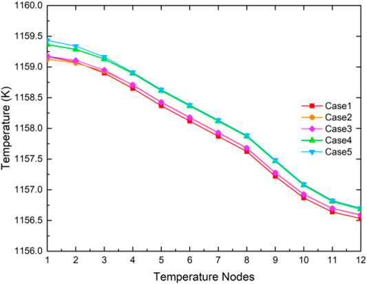
FIGURE 19. Wall temperature distribution in different cases (1).

4.3 Case With Heat Leakage

In a heat pipe cooled reactor, because of the large number of heat pipes used, heat leakage through the insulating layer will be regarded as an important part of the system’s heat dissipation. In this section, the operating characteristics of heat pipes under different heat leakage conditions are preliminarily analyzed. Because of the heat convection between the insulating layer and the environment, obvious condensation between the vapor space and the wick will exist. The latent heat released by condensation will be transferred to the environment through radial heat conduction (Figure 20).

FIGURE 20

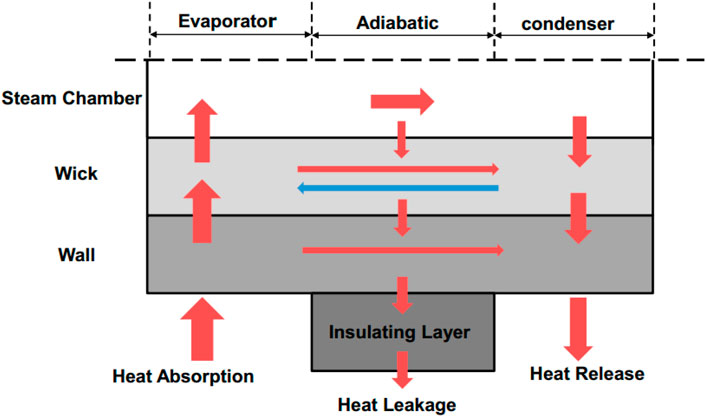
FIGURE 20. Vapor temperature distribution in different cases.

In the calculations, the thermal conductivity of the insulating layer is modified to $3W/\left(m\cdot K\right)$ (case 6), $6W/\left(m\cdot K\right)$ (case 7), and $12W/\left(m\cdot K\right)$ (case 8), respectively. Other parameters remain unchanged.

Figure 21 shows the temperature distribution of the wall in cases of high heat leakage. When heat leakage increases, the operating temperature decreases obviously. Compared with Figure 14, the increase in heat leakage leads to a temperature decrease from about 1160 to 970 K (case 8). Moreover, the heat leakage causes an obvious temperature gradient between the evaporator and the adiabatic section. Because of the poor insulation of the adiabatic section, it can be regarded as the “cold” source and the evaporator is the “heat” source. Therefore, the axial heat conduction causing a significant temperature gradient in the axial direction becomes non-negligible. As for heat conduction between the adiabatic section and the condenser, the temperature difference is inconspicuous because the heat transferred from the evaporator is mainly lost to the environment through the insulating layer rather than to the condenser, leading to a small temperature gradient. If the thermal conductivity of the insulating layer is high enough, the surface temperature in the adiabatic section will be even lower than that of the condenser, resulting in the reverse heat conduction from the condenser to the adiabatic section (cases 7 and 8).

FIGURE 21

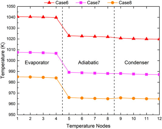
FIGURE 21. Schematic diagram of heat leakage of the heat pipe.

From Figure 22, it can be found that because of the heat leakage, more condensation occurs in the adiabatic section, leading to the decrease of vapor flow in the condenser. The reduction of heat transfer in the condenser is the root cause of the temperature drop of the heat pipe. From these results, it can be concluded that it is essential to keep the heat preservation performance of the heat pipe system.

FIGURE 22

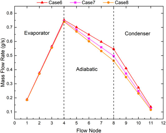
FIGURE 22. Wall temperature distribution in different cases (2).

4.4 Case With Inclined Operation

For mobile power stations such as the eVinci reactor, an inclined operation may occur (Figure 23). In this section, the working medium flow and temperature distribution at different inclined angles are simulated, and the capillary limit of the heat pipe is judged.

FIGURE 23

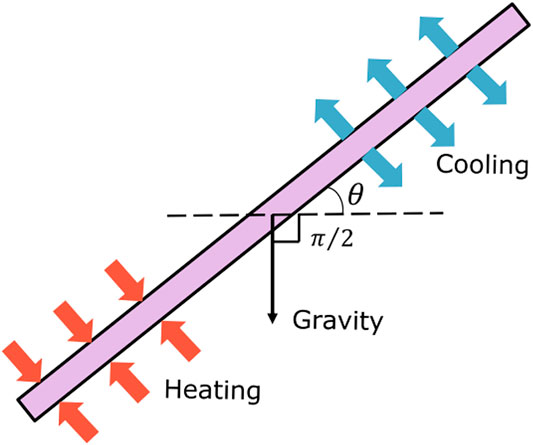
FIGURE 23. Mass flow rate in the vapor space.

From Table 4, the influence of gravity on the flow mainly shows in the pressure drop in the wick, but the influence on the vapor flow is not obvious. It is because the working medium in the wick is a high-density liquid, and the density of the vapor in the vapor space is low enough. When the angle is positive, gravity provides the effective pressure head for the flow, reducing the total pressure drop. The larger the inclination angle of the heat pipe, the more effective the pressure head is provided by gravity. Particularly, when the angle is ${90}^{\circ }$, the pressure drop in the wick is less than that in the vapor space. However, when the angle is negative, the working medium has to overcome the influence of gravity. According to the calculation, when the inclination angle is −30°, the total pressure drop of the working medium exceeds the pumping head of the capillary, and the capillary limit occurs. It should be mentioned that the model is built on the assumption that gravity does not cause the redistribution of the working medium. In fact, this assumption may not be believable at a large inclined angle. When the inclined angle is large enough, the working medium will accumulate at the lower region, resulting in the increase of the working medium in the evaporator and a change in the vapor–liquid interface shape, affecting the actual heat transfer of the heat pipe.

TABLE 4

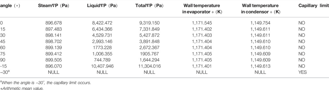
TABLE 4. Pressure drop and heat transfer of a heat pipe at different inclined angles.

5 Conclusion

The accurate calculation of heat pipes will affect the reliability of the analysis results of the heat pipe cooled reactor system. Based on the network method, an improved model is proposed. It can calculate more realistic temperature distributions and obtain information on fluid flow and pressure distribution.

For the high-temperature sodium heat pipe of 1.0 m length, based on the analysis, it can be concluded that non-uniform heating and cooling can change the temperature distribution of the heat pipe. The greater the non-uniformity is, the larger the temperature difference will be. When the heat leakage is obvious, it will not only reduce the operating temperature but also lead to a large temperature gradient between the evaporator and the adiabatic section. As for the gravity term, the influence on the flow depends on the inclination degree. When the angle is positive, gravity will provide an effective pressure head for the flow. When the angle is negative, the fluid needs to overcome its influence. When the inclination angle exceeds $-{30}^{°}$, the heat pipe may reach the capillary limitation, and it may be damaged.

It should be highlighted that gravity may lead to the redistribution of the working medium in the heat pipe, which is ignored in this model. In the future, numerical analyses and experimental investigations of gravity effects on heat pipes will be carried out. Coupling simulation with the reactor core will also be investigated.

Data Availability Statement

The original contributions presented in the study are included in the article/Supplementary Material, further inquiries can be directed to the corresponding author.

Author Contributions

YG and ZL contributed to the conception and design of this study. ZS performed the statistical analysis. All authors contributed to the writing of the manuscript.

Funding

This research was funded by the National Key Research and Development Project of China, (No. 2020YFB1901700), the Science Challenge Project (TZ2018001), Project 11775126/11775127 by the National Natural Science Foundation of China, and the Tsinghua University Initiative Scientific Research Program.

Conflict of Interest

The authors declare that the research was conducted in the absence of any commercial or financial relationships that could be construed as a potential conflict of interest.

The handling editor (FM) declared a past co-authorship with one of the authors (WV).

Publisher’s Note

All claims expressed in this article are solely those of the authors and do not necessarily represent those of their affiliated organizations, or those of the publisher, the editors and the reviewers. Any product that may be evaluated in this article, or claim that may be made by its manufacturer, is not guaranteed or endorsed by the publisher.

References

Alizadehdakhel, A., Rahimi, M., and Alsairafi, A. A. (2010). CFD Modeling of Flow and Heat Transfer in a Thermosyphon. Int. Commun. Heat Mass Transfer 37 (3), 312–318. doi:10.1016/j.icheatmasstransfer.2009.09.002

CrossRef Full Text | Google Scholar

Annamalai, S., and Ramalingam, V. (2011). Experimental Investigation and CFD Analysis of a Air Cooled Condenser Heat Pipe. Therm. Sci. 15 (3), 759–772. doi:10.2298/tsci100331023a

CrossRef Full Text | Google Scholar

Boothaisong, S., Rittidech, S., Chompookham, T., Thongmoon, M., Ding, Y., and Li, Y. (2015). Three-dimensional Transient Mathematical Model to Predict the Heat Transfer Rate of a Heat Pipe[J]. Adv. Mech. Eng. 7 (2), 1687814014567811. doi:10.1177/1687814014567811

CrossRef Full Text | Google Scholar

Bowman, W. J. (1991). Numerical Modeling of Heat-Pipe Transients. J. Thermophys. Heat transfer 5 (3), 374–379. doi:10.2514/3.273

CrossRef Full Text | Google Scholar

Busse, C. A. (1973). Theory of the Ultimate Heat Transfer Limit of Cylindrical Heat Pipes. Int. J. Heat Mass Transfer 16 (1), 169–186. doi:10.1016/0017-9310(73)90260-3

CrossRef Full Text | Google Scholar

Cao, Y., and Faghri, A. (1993). A Numerical Analysis of High-Temperature Heat Pipe Startup from the Frozen State. J. Heat Transfer 115 (1), 247–254. doi:10.1115/1.2910657

CrossRef Full Text | Google Scholar

Cao, Y., and Faghri, A. (1993). Simulation of the Early Startup Period of High-Temperature Heat Pipes from the Frozen State by a Rarefied Vapor Self-Diffusion Model. J. Heat Transfer 115 (1), 239–246. doi:10.1115/1.2910655

CrossRef Full Text | Google Scholar

Cao, Y., and Faghri, A. (1991). Transient Two-Dimensional Compressible Analysis for High-Temperature Heat Pipes with Pulsed Heat Input. Numer. Heat Transfer, A: Appl. 18 (4), 483–502. doi:10.1080/10407789008944804

CrossRef Full Text | Google Scholar

Cotter, T. P. (1965). Theory of Heat pipes[M]. Los Alamos Scientific Laboratory of the University of California.

Google Scholar

El‐Genk, M. S., and Tournier, J. M. (2004). Conceptual Design of HP‐STMCs Space Reactor Power System for 110 kWe[C]. AIP Conf. Proc. Am. Inst. Phys. 699 (1), 658–672.

Google Scholar

El-Genk, M. S., and Lianmin, H. (1993). An Experimental Investigation of the Transient Response of a Water Heat Pipe. Int. J. Heat Mass Transfer 36 (15), 3823–3830. doi:10.1063/1.1649628

CrossRef Full Text | Google Scholar

Faghri, A. (1995). Heat pipe science and technology. Fuel Energy Abst. 36 (4), 285–285. doi:10.1016/0140-6701(95)95609-9

CrossRef Full Text | Google Scholar

Faghri, A., and Harley, C. (1994). Transient Lumped Heat Pipe Analyses. Heat Recovery Syst. CHP 14 (4), 351–363. doi:10.1016/0890-4332(94)90039-6

CrossRef Full Text | Google Scholar

Ferrandi, C., Iorizzo, F., Mameli, M., Zinna, S., and Marengo, M. (2013). Lumped Parameter Model of Sintered Heat Pipe: Transient Numerical Analysis and Validation. Appl. Therm. Eng. 50 (1), 1280–1290. doi:10.1016/j.applthermaleng.2012.07.022

CrossRef Full Text | Google Scholar

Fink, J. K., and Leibowitz, L. (1995). Thermodynamic and Transport Properties of Sodium Liquid and vapor[R]. United States: N. p., 1995. Web. doi:10.2172/94649

CrossRef Full Text | Google Scholar

Huang, L., El-Genk, M. S., and Tournier, J. M. (1993). Transient Performance of an Inclined Water Heat Pipe with a Screen Wick[J]. ASME-PUBLICATIONS-HTD 236, 87.

Google Scholar

Kadak, A. C. (2017). A Comparison of Advanced Nuclear technologies[M]. Columbia University in the City of New York.

Google Scholar

Kim, B. H., and Peterson, G. P. (1995). Analysis of the Critical Weber Number at the Onset of Liquid Entrainment in Capillary-Driven Heat Pipes. Int. J. Heat mass transfer 38 (8), 1427–1442. doi:10.1016/0017-9310(94)00249-u

CrossRef Full Text | Google Scholar

Kumar, S. S., and Ramamurthi, K. (2001). Prediction of Thermal Contact Conductance in Vacuum Using Monte Carlo Simulation. J. Thermophys. Heat transfer 15 (1), 27–33. doi:10.2514/2.6592

CrossRef Full Text | Google Scholar

Levy, E. K., and Chou, S. F. (1973). The Sonic Limit in Sodium Heat Pipes. Heat Transfer 95, 218–223. doi:10.1115/1.3450029

CrossRef Full Text | Google Scholar

Lin, Z., Wang, S., Shirakashi, R., and Winston Zhang, L. (2013). Simulation of a Miniature Oscillating Heat Pipe in Bottom Heating Mode Using CFD with Unsteady Modeling. Int. J. Heat Mass Transfer 57 (2), 642–656. doi:10.1016/j.ijheatmasstransfer.2012.09.007

CrossRef Full Text | Google Scholar

McClure, P., Poston, D., Rao, D., and Reid, R. (2015).Design of Megawatt Power Level Heat Pipe Reactors. Technical Report. Los Alamos, NM (United States): Los Alamos National Lab. LA-UR-15-28840.

Google Scholar

Poston, D. I., Gibson, M., and McClure, P. (2019). “Kilopower Reactors for Potential Space Exploration Missions[C],” in Proceeding of the Nuclear and Emerging Techologies for Space, May 2019 (American Nuclear Society Topical Meeting. ANS.).

Google Scholar

Poston, D. I. (2001). The Heatpipe-Operated Mars Exploration Reactor (HOMER)[C]. AIP Conf. Proc. Am. Inst. Phys. 552 (1), 797–804. doi:10.1063/1.1358010

CrossRef Full Text | Google Scholar

Rice, J., and Faghri, A. (2007). Analysis of Screen Wick Heat Pipes, Including Capillary Dry-Out Limitations. J. Thermophys. Heat transfer 21 (3), 475–486. doi:10.2514/1.24809

CrossRef Full Text | Google Scholar

Song, S., and Yovanovich, M. M. (1988). Relative Contact Pressure - Dependence on Surface Roughness and Vickers Microhardness. J. Thermophys. Heat transfer 2 (1), 43–47. doi:10.2514/3.60

CrossRef Full Text | Google Scholar

Swartz, M. M., Byers, W. A., Lojek, J., and Blunt, R. (2021). “Westinghouse eVinci™ Heat Pipe Micro Reactor Technology Development[C],” in International Conference on Nuclear Engineering, October 2021 (American Society of Mechanical Engineers), 85246. V001T04A018.

Google Scholar

Tournier, J.-M., and El-Genk, M. S. (1994). A Heat Pipe Transient Analysis Model. Int. J. Heat Mass Transfer 37 (5), 753–762. doi:10.1016/0017-9310(94)90113-9

CrossRef Full Text | Google Scholar

Tournier, J. M., and El-Genk, M. S. (1996). A Vapor Flow Model for Analysis of Liquid-Metal Heat Pipe Startup from a Frozen State. Int. J. Heat mass transfer 39 (18), 3767–3780. doi:10.1016/0017-9310(96)00066-x

CrossRef Full Text | Google Scholar

Xu, J. L., and Zhang, X. M. (2005). Start-up and Steady thermal Oscillation of a Pulsating Heat Pipe. Heat Mass. Transfer 41 (8), 685–694. doi:10.1007/s00231-004-0535-3

CrossRef Full Text | Google Scholar

Yuan, Y., Shan, J., Zhang, B., Gou, J., Zhang, B., Lu, T., et al. (2016). Study on Startup Characteristics of Heat Pipe Cooled and AMTEC Conversion Space Reactor System. Prog. Nucl. Energ. 86, 18–30. doi:10.1016/j.pnucene.2015.10.002

CrossRef Full Text | Google Scholar

Yue, C., Zhang, Q., Zhai, Z., and Ling, L. (2018). CFD Simulation on the Heat Transfer and Flow Characteristics of a Microchannel Separate Heat Pipe under Different Filling Ratios. Appl. Therm. Eng. 139, 25–34. doi:10.1016/j.applthermaleng.2018.01.011

CrossRef Full Text | Google Scholar

Zuo, Z. J., and Faghri, A. (1998). A Network Thermodynamic Analysis of the Heat Pipe. Int. J. Heat Mass Transfer 41 (11), 1473–1484. doi:10.1016/s0017-9310(97)00220-2

CrossRef Full Text | Google Scholar

Nomenclature

$A$ area $\left(m^2\right)$

$C$ specific heat capacity $\left(J/\left(kg\cdot K\right)\right)$

$\text{g}$ acceleration of gravity $\left(m/s^2\right)$

$h$ specific enthalpy $\left(J/kg\right)$

$k$ heat conductivity $\left(W/\left(m\cdot K\right)\right)$

$K$ permeability

$L$ length $\left(m\right)$

$P$ pressure $\left(Pa\right)$

$q$ mass flow rate $\left(kg/s\right)$

$Q$ heating power $\left(W\right)$

$r$ radius $\left(m\right)$

$R$ thermal resistance $\left(K/W\right)$

$R_g$ gas constant $\left(J/\left(kg\cdot K\right)\right)$

$T$ temperature $\left(K\right)$

$Thick$ thickness $\left(m\right)$

$u$ velocity $\left(m/s\right)$

$V$ volume $\left(m^3\right)$

$\rho$ density $\left(kg/m^3\right)$

$\mu$ dynamic viscosity $\left(Pa\cdot m\right)$

$\epsilon$ porosity

$\lambda$ convective heat transfer coefficient $\left(W/\left(m^2\cdot K\right)\right)$

$\gamma$ heat capacity ratio

$\mathit{Y}$ variable vector

$\mathit{b}$ weight coefficient vector

$\mathit{\tau }$ node coefficient vector

$\mathit{a}$ coefficient matrix

Subscripts

$pe$ wall region in the evaporator/radial direction (1)

$pr$ radial direction (2)

$pc$ wall region in the condenser/radial direction (3)

$we$ wick region in the evaporator/radial direction (4)

$wr$ radial direction (5)

$wc$ wick region in the condenser/radial direction (6)

$pa$ wall region in the adiabatic section/axial direction (1)

$wa$ wick region in the adiabatic section/axial direction (2)

$ve$ vapor space region in the evaporator

$va$ vapor space region in the adiabatic section

$vc$ vapor space region in the condenser

$in$ insulating layer/inner radius/heat absorption

$gap$ contact gap

$evap$ evaporation evaporator

$cond$ condensation condenser

$mv$ mass flow rate of vapor

$ml$ mass flow rate of liquid

$out$ outer radius

$equ$ equivalent parameter

$eff$ effective parameter

$evap$ evaporation evaporator

$adia$ adiabatic section

$cond$ condensation condenser

$f$ fluid

$v$ vapor

$w$ wick mesh

$c$ capillary