A Study on Nexus Between Renewable Energy and Fossil Fuel Consumption in Commercial Sectors of United States Using Wavelet Coherence and Quantile-on-Quantile Regression

The inertia of fossil fuels in the commercial sector of the United States has maintained its momentum throughout, and efforts to replace it with renewable energy has continuously been made. This dynamic relationship is impacted by multi-economic and political variables both in the domestic and international markets. In this paper, we have explored the dynamic impact of total renewable energy consumption (RE) on the decomposed wavelet frequencies of energy consumed by fossil fuels (FE) in the commercial sectors of the United States economy. In particular, we have applied wavelet coherence and quantile-on-quantile regression methodologies to evaluate this relationship. The monthly data from the US Energy Information Administration over a period of January 2001 to July 2021 was procured for the present study. Our empirical findings based on wavelet coherence showed significant co-movements between FE and RE with positive association in short-run while negative association in long-run monthly frequency bands. For our five models based on quantiles and decomposed wavelet frequencies of FE, four models show that renewable energy consumption has an antagonistic relation with the FE in the commercial sector of the United States.

Introduction

Carbon emissions have reached questionable levels globally (Garrett-Peltier, 2017). It has been estimated that globally, energy requirements are going to increase by over 44% in the first three decades of the century. Nevertheless, by 2030, 80% of the energy will still be non-renewable in nature (Akorede et al., 2010). The United States, with close to 4% of the global population, contributes ∼14% of the global emissions (Dogan and Ozturk,2017). Development at this cost, scale, and style has a tendency to jeopardize the environment (Ramzan et al., 2022).

In the United States, non-renewable energy is usually derived from non-replenishable sources such as natural gas, coal, and petroleum, while renewable energy sources include replenishable sources such as solar photovoltaic, biomass wood, biomass waste, hydropower, wind, nuclear, and geothermal. Furthermore, the commercial sector can be classified as businesses and establishments that do not include non-manufacturing, e.g., restaurants, the service sector, software firms, banks, education organizations, etc. (Agarwal et al., 2010).

It is expected that towards the end of the 21st century, the American commercial energy blend will have material contributions from renewable energy (Klass,2003). The National Energy Model is a powerful model that trails the essential energy sources and their usage by families and commercial establishments; this has been implemented in Japan as well. The inspiration driving the advancement of this energy economic model in America has been the need for a system that would evaluate the consequences for the United States economy of strategy changes in the utilization of fuel sources from petroleum derivatives to renewables to accomplish the objective of calibrating greenhouse gas over the next 5 decades (Agarwal et al., 2010; Nakata, 2004). While support from the government is the most import propellant increasing investments in renewable energy, it is widely accepted that government policies are never unidimensional and have employment generation at their heart. Based on this parameter, one has to see the development of jobs created by industries supported by energy from fossil fuels and those using energy from renewable sources. This becomes another reason determining the dynamics between the two variables (Peltier et al., 2014).

Table 1 shows that over the past 2 decades, the contribution to the primary energy consumption in the commercial sector in the United States has more than doubled from 2.5% in 2001 to 6.6% in 2020; nonetheless, the contribution still remains abysmally low. The CAGR in the renewable energy consumed by the commercial sector over 2 decades is 5.66% in comparison to a 0.35% CAGR in the total primary energy consumed by the commercial sector. At this rate, the total renewable energy consumed by the commercial sector can double in a little over 12 years. This growth will mainly come from solar or wind, as most of the sites for hydropower have been utilized (Cameron et al., 2001; Cai et al., 2018).

TABLE 1

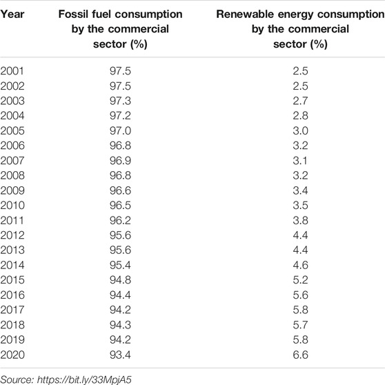
TABLE 1. Total primary energy consumed by the commercial sector.

Similar studies in China have shown that the impact of renewable energy on phasing out energy consumed by fossil fuels depends on the subsidies provided by the government (Cabré et al., 2018; Ouyang and Lin, 2014). Studies in India on similar variables show that while the country had the potential for renewable energy, government policy and support were needed for renewable energy to make inroads in the non-renewable energy territory (Solarin and Bello, 2021). In smaller developing nations like Malaysia, despite having a large hydropower potential, close to only 10% of the total reserves have been harnessed. Even its large biomass reserve of palm oil has not been harnessed (Ong et al., 2011). On the contrary, in the USA’s neighbor, Mexico, the congress has planned that the non-renewable energy source-based power be restricted to 65% by 2024, 60% by 2035, and half by 2050 (Cai et al., 2018; Vidal-Amaro et al., 2015). It is estimated that biomass can reduce greenhouse emissions by close to 18% in Mexico (Tauro et al., 2018). In developed nations such as Japan, where the commercial sector consumes ∼22% of the energy, renewable energy contribution is less than 5% (Konstantin, 2017).

Time and again, the fragility and the overdependence of the American economy on non-renewable energy have been highlighted every time there has been a crude oil crisis. While the need for renewable energy is clearly understood and defined, its efficiency when compared to non-renewable energy is a key factor contributing to the dynamics between the two sources of energy (Koroneos et al., 2003; Oró et al., 2015).

Another factor impacting the relationship and dynamics between total renewable energy consumption and energy consumed by fossil fuels is the need for dependable power during working hours of the commercial sectors in the United States. Solar and wind power are not dependable sources of power, and the fluctuations in this type of electricity generation may not be synchronized with the continuous demand with the load dispatch centers (Perez et al., 1990; Yang et al., 2008). The geophysical restraints of renewable sources of energy become another factor impacting their dynamics in comparison with the energy consumed by fossil fuels (Shaner et al., 2018). To counter the solar cycles, more blended co-generation plants need to be evaluated so as to increase the efficiency and dependability of the renewable energy sources of energy as compared to the non-renewable energy sources (Dunham and Iverson, 2014; Gueymard and Ruiz-Arias, 2016).

At the same time, many factors impact the shift or simply the adoption of green energy in businesses in the United States, e.g., clean/green energy policies, tax structures and incentives for using clean energy, and economic and political views of the governing bodies (Pahle et al., 2016; Pfeiffer et al., 2016). While analyzing the causal relationship between renewable energy and fossil fuel consumption and growth, bidirectional Granger causality was found to exist between commercial energy consumption and real GDP (Alola and Yildrim, 2019).

Another key element determining the relationship between the total renewable energy consumption (RE) and energy consumed by fossil fuels (FE) is the infrastructure in buildings housing commercial establishments. Sustainable grid connectivity to support the two-way metering and the dependability aspect of clean energy causes a shift from non-renewable energy to green energy (Mbungu et al., 2020). Smart grids also support the switch from FE consumption to RE (Hafeez et al., 2018; Li and Dong, 2016).

Thus, we see that the factors impacting the relationship between the total renewable energy consumption and energy consumed by fossil fuels in commercial sectors in the United States are impacted by numerous factors. While a push from the government in the form of policy and subsidies remains a primary propellent, the comparison of the efficiency of the two sources becomes a major point of contention. Overcoming geophysical restraints and evaluating various blends to increase the dependability of renewable energy supply are other key factor. A key gap that we observe is that of the literature available; most of the studies on the dynamics between RE and FE are focused on developing nations, India and China in particular. Very few studies focus on the developed nations, the United States in particular. At the same time, studies focusing on the dynamics between the two variables in the United States do not focus on the split of the energy consumption. Negligible studies are available focusing on energy dynamics in housing, commercial, and industrial sectors separately. Such a study becomes imperative to understand the microdynamics of the energy demand and synchronize the growth and replacement of energy in this segment with clean energy so as to make growth sustainable and clean (Yi, 2014). In terms of the methodology used, we were yet to come across a study analyzing the nexus between the variables under study using the wavelet coherence and quantile-on-quantile regression methods. The above observations encourage us to evaluate the relationship between renewable energy consumption and energy consumed by fossil fuels in the commercial sector for the United States by applying wavelet coherence and quantile-on-quantile regression.

Data

The present study discusses the relationship between RE consumption and FE in commercial sectors of the United States by applying wavelet coherence and quantile-on-quantile regression (QQR) methodologies. The sample dataset considers monthly data collected between time periods January 2001 and July 2021. The description and source of data are given in Table 2.

TABLE 2

TABLE 2. Variables and source of data covered.

We aim to study the following in our present study:

(1) The correlation between the variables RE and FE by applying bi-wavelet coherence.

(2) The dynamic impact of RE on decomposed wavelet frequencies of FE by applying the QQR methodology.

Methodology

Multiscale Wavelet Decomposition

The wavelet methodology decomposes the time series into several wavelet frequencies. These wavelets offer frequency decomposition of the time series by preserving time location and thus captures the complete information contained in time series specific to location-scale domain (Ramsey, 1999).

Any function can be decomposed into father ($\varphi )$ and mother ($\psi )$ wavelets (Ramsey, 2002). The father wavelets generate scaling coefficients representing very long scale smooth components, while mother wavelets generate differencing coefficients representing the deviations from the smooth components.

For any function $\varphi (.),$ the father wavelets are defined as follows:

${\varphi }_{M,n}=2^{-M/2}\varphi \left(\frac{t-2^{M}n}{2^M}\right)with\int \varphi \left(t\right)dt=1(1)$

with smooth coefficients defined as

$s_{M,n}=\int f\left(t\right){\varphi }_{M,n}(2)$

Similarly, the mother wavelets are defined as follows:

${\psi }_{m,n}=2^{-m/2}\psi \left(\frac{t-2^{m}n}{2^m}\right) , m=\mathrm{1,2},\dots ,M with \int \psi \left(t\right)dt=0(3)$

with detail coefficients defined as

$d_{m,n}=\int f\left(t\right){\psi }_{m,n}, m=\mathrm{1,2},\dots ,M(4)$

The function $f(.)$ is defined as follows:

$f\left(t\right)=S_M+D_M+D_{M-1}+\dots +D_m+\dots +D_1$

where

$S_M={\displaystyle \sum }_n{s}_{M,n}{\varphi }_{M,n}\left(t\right)and{D}_m={\displaystyle \sum }_n{d}_{m,n}{\psi }_{m,n}\left(t\right), m=\mathrm{1,2},\dots ,M$

The term $S_m$ represents the cumulative sum of variations at scale ${\theta }_m$ with changes in series at $m^{th}$ level wavelet denoted by $D_m$ (Gencay et al., 2001; Ramsey 2002). The scaling and differencing coefficients were calculated using the maximal overlap discrete wavelet transform (MODWT), as there is no restriction on the sample size. Furthermore, the MODWT uses moving differencing and average operator and preserves the sample size at each scale of wavelet decomposition (Percival and Walden 2000).

The Daubechies least asymmetric filter of length eight [LA (8)] is used to disintegrate the series into the wavelet coefficients $D_m$ with a resolution of data at scale $2^m to 2^{m+1}$. The wavelet scales ${\theta }_1, {\theta }_2, {\theta }_3, {\theta }_4$ are associated with oscillation of periods of 2–4, 4–8, 8–16, and 16–32 months, respectively. The long-term movements are denoted by wavelet smooth S4.

Bi-Wavelet Coherence

The wavelet coherence is employed to analyze the periodic phenomena in the presence of sudden changes in frequency across time of a time series. It measures the level and extent of co-movements between time–series pair, say Y and X, but in time–frequency (location–scale) domain and is analogous to traditional bi-variate correlation coefficient.

We define the bi-wavelet coherence as follows:

$R_{yx}= \frac{\nu \left[\mathit{\varrho }\left(y,x\right)\right]}{\sqrt{\nu \left[\mathit{\varrho }\left(y\right)\right].\mathit{\varrho }\left[\omega \left(x\right)\right]}}(5)$

$R_{yx}^2=R_{yx} .R_{yx}^{\ast }$

where $R_{yx}$ is the measure of wavelet coherence between the two time–series Y and X with measure of squared wavelet coherence given by $R_{yx}^2$.

$\mathit{\varrho }(y,x)$ is the cross-wavelet defined by the following:

$\mathit{\varrho }(y,x)=\mathit{\varrho }\left(y\right)\ast \overline{\mathit{\varrho }}\left(x\right)$

with corresponding wavelet transforms $\mathit{\varrho }(.)$ and complex conjugate wavelet transform $\mathit{\varrho }(.)$. $\nu$ is the smoothening operator with desired time–frequency resolution (Torrence and Compo 1998). The wavelet coherence is a measure of the cross-correlation between two time series and ranges between 0 and 1, with values closer to 1 indicating higher correlation.

Quantile-On-Quantile Regression Methodology

Traditionally, the relationship between response (R) and predictor (P) variables is studied by applying a linear regression framework. In recent years, the quantile regression analysis (QR) introduced by Koenker and Bassett (1978) has become a popular tool in modelling the time-varying degree and structure of dependence as they provide more precise and accurate results as compared to linear regression. Furthermore, the robustness of QR to provide tail dependence information (i.e., upper and lower tails) in addition to the median proves its advantage over linear or non-linear regression analysis.

QR approach has one drawback, which is its inability to capture the entire dependence structure. Hence, to overcome this, quantile-on-quantile regression was introduced.

The QQR models the quantile of response (R) variable as a function of quantile of predictor (P) and hence giving the complete dependence structure (Sim and Zhou 2015). The QQR methodology empirically justifies the conditional quantile relationship between variables and can be considered as an extension of QR in the non-parametric set-up. It captures the possible non-stationarity in the series and explains the entire dependent structure instead of interpretation based on point estimation used in classical linear regression, thus minimizing the loss of information.

The QQR model for qq-quantile of response (R) variable as a function of predictor (P) variable and lagged R is defined as follows:

$R_t={\text{α}}^q\left(P_t\right)+{\gamma }^q{P}_{t-1}+{\epsilon }_t^q(6)$

where ${\epsilon }_t^q$ is an error term with zero q-quantile. To examine the dependence structure between q-quantile of R and p-quantile of P ($P^p)$, we linearize the unknown link function ${\text{α}}^q(.)$ using first-order Taylor expansion as follows:

${\text{α}}^q\left(P_t\right)\approx {\text{α}}^q\left(P^p\right)+{\text{α}}^{q\prime }\left(P\right)\left(P_t-P^p\right)(7)$

Following the method of Sim and Zhou (2015), Eq. 7 can be rewritten as follows:

${\text{α}}^q\left(P_t\right)\approx {\text{α}}_0\left(q,p\right)+{\text{α}}_1\left(q,p\right)\left(P_t-P^p\right)(8)$

Eq. 6 reduces to

$R_t={\text{α}}_0\left(q,p\right)+{\text{α}}_1\left(q,p\right)\left(P_t-P^p\right)+\gamma \left(q\right)R_{t-1}+{\epsilon }_t^q(9)$

$R_t=\underset{\ast }{\underset{�}{{\text{α}}_0+{\text{α}}_1\left(P_t-P^q\right)+\gamma \left(q\right)R_{t-1}}}+{\epsilon }_t^q(10)$

where $\gamma \left(q\right)={\gamma }^q, {\text{α}}_0={\text{α}}_0\left(q,p\right) and {\text{α}}_1={\text{α}}_1\left(q,p\right)$

Part (*) in Eq. 10 denotes the qth conditional quantile of response time series variable R and captures the relationship between q-quantile of R and p-quantile of P as ${\text{α}}_0 \& {\text{α}}_1$ are indexed in both q and p. Hence, the complete dependence structure between R and P is determined by the quantile-on-quantile regression model through dependence between their respective distributions.

The estimate of Eq. 10 is obtained by minimizing the following equation:

$\underset{{\text{α}}_0{\text{α}}_1}{\min }{\displaystyle \sum }_{i=1}^n{\varnothing }_q\left[R_t-{\text{α}}_0-{\text{α}}_1\left(P_t-P^p\right)-\gamma \left(q\right)R_{t-1}\right]\ast Q\left(\frac{G_n\left(P_t\right)-p}{h}\right)$

where ${\varnothing }_q$ corresponds to absolute value function, which gives the q conditional quantile of R as a solution. Then the Gaussian kernel Q (.) is conducted to weigh the observation according to normal probability distribution based on bandwidth h. Based on previous studies, a bandwidth of 5% (h = 0.05) was selected (Sim and Zhou 2015). The empirical distribution function is estimated as follows:

$Q_n\left(P_t\right)=\frac{1}{n}{\displaystyle \sum }_{k=1}^{n}I({\widehat{P}}_k<{\widehat{P}}_t)$

The weights are reversely linked to the distance of $G_n\left(P_t\right)$ from p, where p is the value of distribution function corresponding to $P^p$.

Empirical Results

The descriptive statistics of variables—FE and RE—in the commercial sector are given in Table 3.

TABLE 3

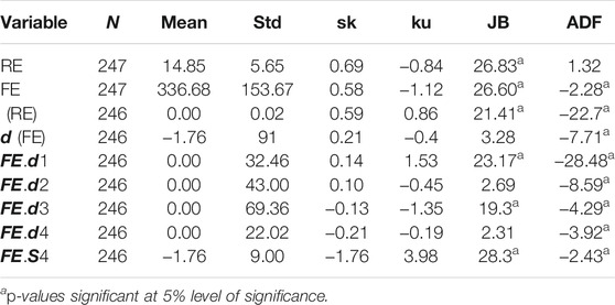
TABLE 3. Descriptive statistics.

As observed from the results of the Jarque–Bera test for normality and the augmented Dickey–Fuller (ADF) test of stationarity in Table 3, the variables FE and RE were observed to be non-normally distributed and non-stationary and hence were transformed. The first difference of FE (dFE) and the first difference of natural logarithm of RE [ (RE)] were used for analysis. The $d$[$d$ (FE)] were further decomposed into wavelet frequencies denoted by FE. d1, FE. d2, FE. d3, FE. d4, and FE. S4 corresponding to 2–4, 4–8, 8–16, and 16–32 months and the long-term trend, respectively.

The summary statistics as reported in Table 3 clearly show non-normal distributions for the variables, and the results of BDS test for non-linearity as stated in Table 4 indicate that the OLS estimates will be unreliable and hence provide a good motivation to apply a quantile-based approach to accommodate for the heavy tails.

TABLE 4

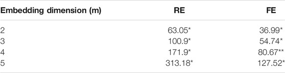
TABLE 4. BDS test of non-linearity of residuals.

For our objective 1, the wavelet coherence methodology was applied to study the co-movement between RE and FE in commercial sectors of the United States.

The warmer (colder) colors, red (blue), indicate strong (weak) significant co-movements between the series. The estimates of wavelet coefficients are statistically insignificant beyond the black line cone at 5% level of significance. The lead/lag phase relations between the series are indicated by arrow directions. Arrows pointing towards the right (left) represent the series that are in-phase (out-phase), indicating positive (negative) coherence/correlation. Arrows pointing right-down or left-up indicate that the second series is leading, while arrows pointing left-down or right-up indicate that the first series is leading.

From Figure 1, a significant coherence is observed in 1–2 and 2–4 frequency bands at few time-points, and variables are observed mostly in-phase (positively correlated). Furthermore, a huge island of significant coherence is observed in 4–8 and 8–16 frequency bands, indicating a long-term impact with variables being out-phase (negatively correlated).

FIGURE 1

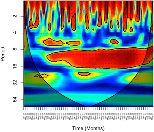
FIGURE 1. Bi-wavelet coherence.

This time-frequency dependence between RE and FE in the commercial sector is further studied in detail by applying the QQR methodology (objective 2). The impact of RE on each frequency bands of FE , FE. d1, FE. d2, FE. d3, FE. d4, and FE. S4 is studied in detail by implementing the QQR methodology on each of the frequency bands.

Based on the QQR model expressed in Eq 10, the following QQR fit models are considered in our present analysis to study the effect of RE consumption on energy consumed by fossil fuel bands (FE.d1, FE. d2, FE.3,FE.4, and FE. S4) in the commercial sector:

$M-1: FE.d{1}_t={\text{α}}_0\left(q,p\right)+{\text{α}}_1\left(q,p\right)\left(R{E}_t-R{E}^p\right)+\gamma \left(q\right)FE.d{1}_{t-1}+{\epsilon }_t^q$

$M-2: FE.d{2}_t={\text{α}}_0\left(q,p\right)+{\text{α}}_1\left(q,p\right)\left(R{E}_t-R{E}^p\right)+\gamma \left(q\right)FE.d{2}_{t-1}+{\epsilon }_t^q$

$M-3: FE.d{3}_t={\text{α}}_0\left(q,p\right)+{\text{α}}_1\left(q,p\right)\left(R{E}_t-R{E}^p\right)+\gamma \left(q\right)FE.d{3}_{t-1}+{\epsilon }_t^q$

$M-4: FE.d{4}_t={\text{α}}_0\left(q,p\right)+{\text{α}}_1\left(q,p\right)\left(R{E}_t-R{E}^p\right)+\gamma \left(q\right)FE.d{4}_{t-1}+{\epsilon }_t^q$

$M-5: FE.S{4}_t={\text{α}}_0\left(q,p\right)+{\text{α}}_1\left(q,p\right)\left(R{E}_t-R{E}^p\right)+\gamma \left(q\right)FE.S{4}_{t-1}+{\epsilon }_t^q$

The results of the QQR analysis can be summarized by two parameters: ${\text{α}}_0={\text{α}}_0\left(p,q\right) and {\text{α}}_1={\text{α}}_1\left(p,q\right)$, which is the intercept term and the slope coefficient, respectively. The results of intercept (${\text{α}}_0$) and slope coefficients $\left({\text{α}}_1\right)$ for quantiles between 0.05, 0.10, … , and 0.95 are presented in Figures 2–6 for QQR model fit with bandwidth, h = 0.05. The first column represents the QQR model fit of response variable (R) on the predictor (P), the second column represents the intercept ${\text{α}}_0$, and the third column explains the slope coefficients $\left({\text{α}}_1\right)$ at quantile levels = 0.05, 0.10, … , and 0.95.

FIGURE 2

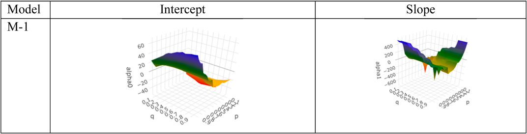
FIGURE 2. Quantile-on-quantile regression(QQR) estimates for Model 1.

For Model 1, the QQR slope coefficients were negative for lower quantiles, [0.05–0.35], of renewable energy consumption and for the quantile range [0.35–0.65] of energy consumed by FE. d1, indicating that, as the renewable energy consumption increased, the energy consumed by fossil fuels decreased for lower concentrations of renewable energy consumption in 2–4 frequency band. The coefficients were positive for all quantiles greater than 0.7 of energy consumed by FE. d1 (Figure 2). For QR regression fit, the slope coefficients were found to be negative in quantile grid [0.2–0.7] and significant for the quantiles [0.35–0.5, 0.65]. A similar trend can be observed from Figure 1 of wavelet coherence.

For Model 2, the QQR slope coefficients were negative for all quantiles of renewable energy consumption and for quantile range [0.4–0.55] of energy consumed by FE. d2, indicating that, as the renewable energy consumption increased, the energy consumed by fossil fuels decreased for all concentrations of renewable energy consumption in the 4–8 frequency band (Figure 3). For QR regression fit, the slope coefficients were found to be negative in the quantile grid [0.05–0.95] and significant for the quantiles [0.4–0.6, 0.65]. A similar trend can be observed from Figure 1 of wavelet coherence.

FIGURE 3

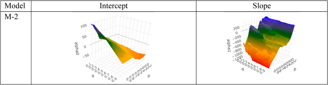
FIGURE 3. QQR estimates for Model 2.

For Model 3, the QQR slope coefficients were negative for almost all quantiles of renewable energy consumption and of energy consumed by FE. d3, indicating that, as the renewable energy consumption increased, the energy consumed by fossil fuels decreased for all concentrations of renewable energy consumption in the 8–16 frequency band (Figure 4). For QR regression fit, the slope coefficients were found to be negative in the quantile grid [0.05–0.95] and significant for all the quantiles except at 0.75 and 0.95. A similar trend can be observed from Figure 1 of wavelet coherence.

FIGURE 4

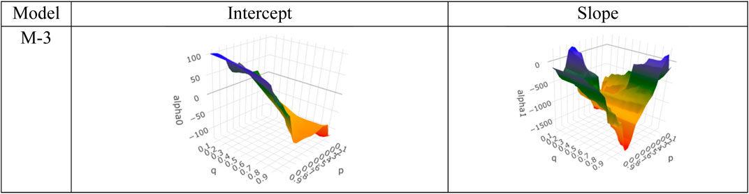
FIGURE 4. QQR estimates for Model 3.

For Model 4, the QQR slope coefficients were positive for all quantiles of renewable energy consumption and of energy consumed by FE. d4, indicating that, as the renewable energy consumption increased, the energy consumed by fossil fuels increased for all concentrations of renewable energy consumption in the 16–32 frequency band (Figure 5). For QR regression fit, the slope coefficients were found to be positive in the quantile grid [0.05–0.95] and non-significant for lower and upper tails.

FIGURE 5

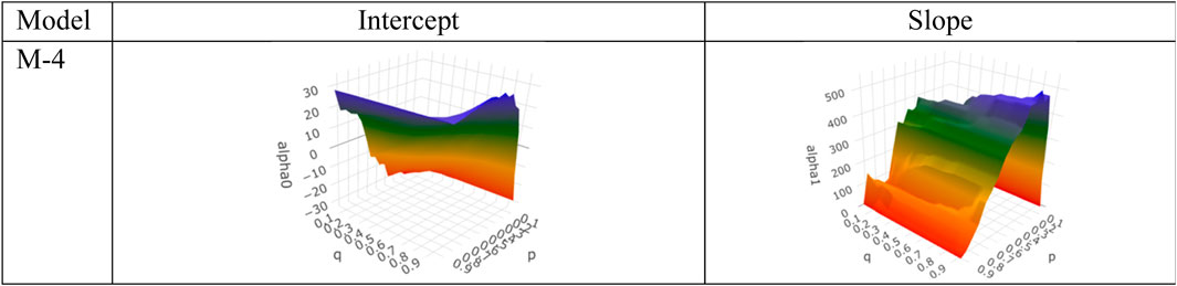
FIGURE 5. QQR estimates for Model 4

For Model 5, the QQR slope coefficients were negative for most of the quantiles of renewable energy consumption and of energy consumed by FE. S4, indicating that, as the renewable energy consumption increased, the energy consumed by fossil fuels decreased for all concentrations of renewable energy consumption for long-term trend. For QR regression fit, the slope coefficients were found to be negative in the quantile grid [0.05–0.95] but non-significant.

The linear quantile regression model is defined as follows:

$R_t^q={\beta }_0^q+{\beta }_1^q{P}_t+{\beta }_2^q{R}_{t-1}^q+{\epsilon }_t^q(11)$

where $R_t^q$ is the qth conditional quantile of dependent variable, the parameter ${\beta }_0^q={\beta }_0$ is the intercept, and the regression estimator ${\beta }_1^q={\beta }_1$ is the function of q.

The QQR estimates decompose QR estimates specific for different quantiles of response variables. The QR approach regresses the qth quantile of response variable, whereas the QQR approach regresses the qth quantile of predictor variable on the pth quantile of response variable, and as a result, its parameters are functions of (q, p). Hence, the QQR method conveys more information about the relationship between predictor and response variable as compared to QR approach.

The following relationships hold for QR and QQR estimates:

${\widehat{\beta }}_0=\frac{1}{m}{\displaystyle \sum }_p{\widehat{\alpha }}_0={\widehat{\overline{\alpha }}}_0 and {\widehat{\beta }}_{1j}=\frac{1}{m}{\displaystyle \sum }_p{\widehat{\alpha }}_1={\widehat{\overline{\alpha }}}_1$

where j = 1, 2 and m and m are the number of points of the quantile grid q = (0, 1).

Hence, the averaged QQR estimates should be equal to QR estimates.

The graphs of comparison are presented in Figure 7, showing the average QQR estimates of the slope coefficients (${\widehat{\overline{\alpha }}}_1$) and QR estimates of the slope (${\widehat{\beta }}_{1j}$) for all the pairs over the quantile grid [0.05, 0.10, … , 0.95].

FIGURE 7

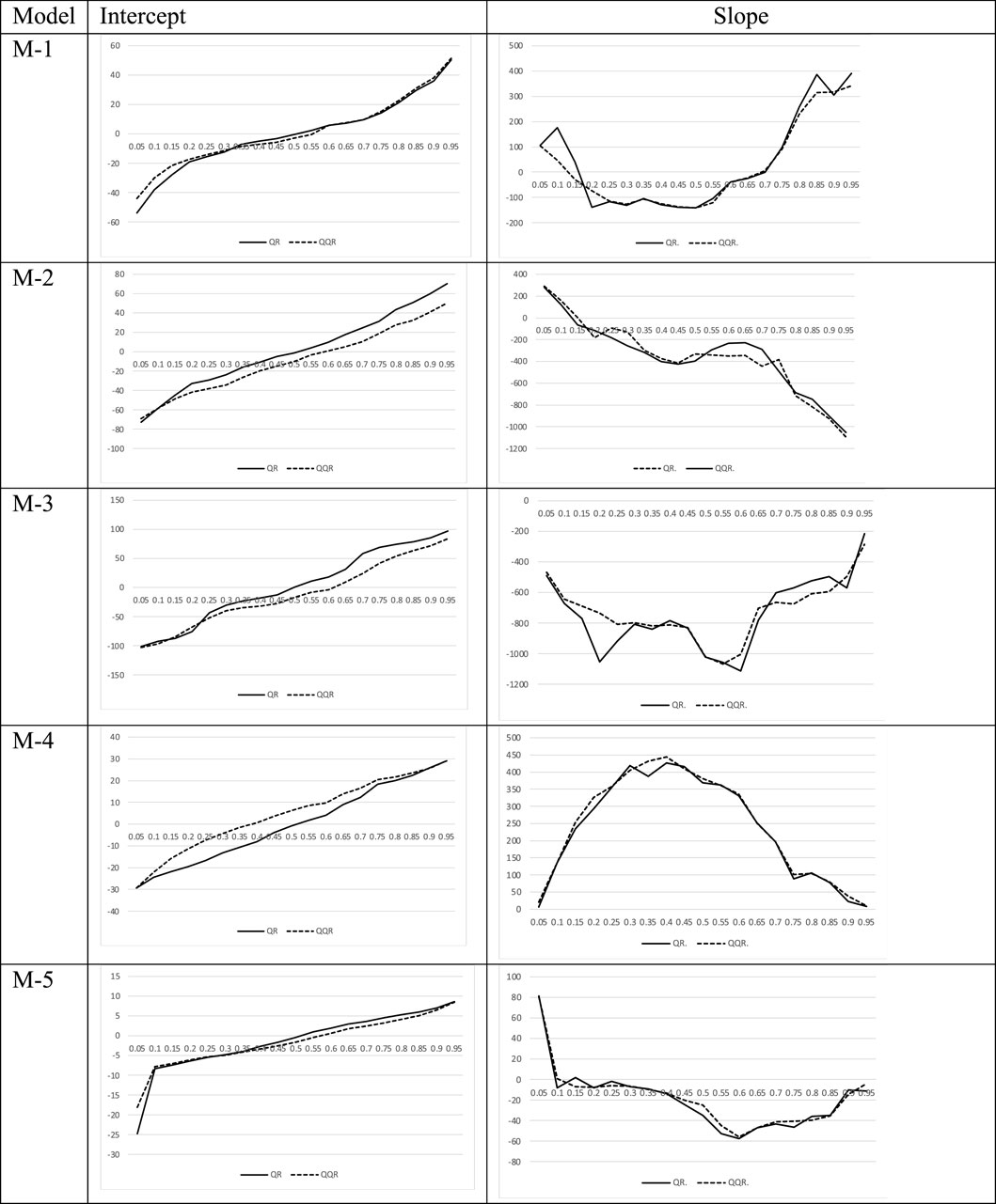
FIGURE 7. Quantile regression analysis(QR) vs QQR estimates.

As observed from Figure 7, the estimates of QQR and QR regression were found to be similar for all the models, indicating a good fit and validity of our QQR methodology.

Discussion

As discussed above, the collected monthly data on FE is decomposed into five frequency components using wavelets. The summary statistics reported in Table 3 indicate non-normality for the variables and motivate us to rely primarily on a quantile-based approach. Furthermore, the BDS test of non-linearity as reported in Table 4 indicates that the ordinary least estimates (OLS) will not be reliable to detect the relationship between FE and RE. The co-movements as indicated by Figure 1 show that the two variables are in-phase (positively correlated) in the short run, while they are out-phase (negatively correlated) in the long run at 5% level of significance. The impact of RE on the decomposed frequencies of FE is observed to be negative and significant at the 5% level of significance in most cases as can be observed from the results of quantile regression and quantile-on-quantile regression fit models 1–5.

For shorter frequencies (2–4 months), a negative and significant impact of RE was observed in the quartile range [0.35–0.5]. Furthermore, for longer frequencies (4–8 and 8–16 months), a similar negative and significant impact of RE was observed on FE. A positive correlation was observed between RE and FE in 16–32-month frequency band but was observed to be insignificant. In the long-term, a negative impact of RE was observed on FE but was insignificant, indicating that increased RE consumption will not cause a deterioration in FE in commercial sector in the long run. Our results highlight the importance of not only studying the entire conditional distribution of FE (based on quantile regression) but also looking at the various frequencies.

The quantile-on-quantile regression gives further insights into the analysis whether there is also a role for various levels of RE in the conditional distribution behavior of FE and its various frequencies. The results of intercept and slope coefficients are depicted in Figures 2–6 using three-dimensional graphs. We observe that quantile regression results carry over to the quantile-on-quantile regression results for shorter as well as longer frequencies of FE with the relationship being mostly negative with RE. In long-term frequency band, a significant negative coherence is observed between the two variables, indicating that the renewable energy consumption has a significant negative impact on energy consumed by fossil fuels in the commercial sector. Furthermore, the validity of quantile-on-quantile regression fits was checked with that of quantile regression estimates. The similarity in the trend of plots of intercept and slope coefficients of quantile regression vs averaged quantile-on-quantile regression estimates presented in Figure 7 depicted the goodness of fit of quantile-on-quantile regression methodology.

FIGURE 6

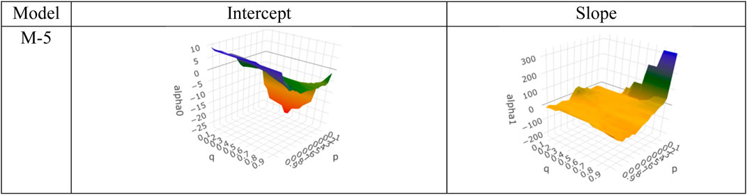
FIGURE 6. QQR estimates for Model 5.

Conclusion and Policy Implication

There is no taking from the fact that based on the data shared in this study and the analysis presented, the usage of renewable energy has been comparatively small in the United States in comparison to the non-renewable fossil fuels in the commercial sector in United States. Notwithstanding the realities that exhibited advancements for using RE assets are plentiful, fossil energy utilization keeps on expanding at a scale that cannot be supported in the US, and sustainable commitments to energy efficiency are yet to catch the pace they need to catch. It is but inevitable that the replenishment of fossil fuels is not possible; however, in the short and medium run, the actual implication of this adage is far from visible in the United States in terms of the quantum and pace that are required to maintain the sustainability of the environment. The best propellant for this could be the retail price of fossil fuels becoming exorbitantly high excessively and irreversibly in the hands of the commercial consumer.

The present study investigated the implications of renewable energy consumption on the fossil fuel-based energy in the commercial sector in the United States using monthly frequency data for a period of January 2001–July 2021. We applied wavelet coherence and quantile-on-quantile regression methodologies on decomposed wavelet frequencies of FE to assess the relationship between the latter and that of various quantiles of RE. Based on empirical results, we arrive at the conclusion that a positive association in the short run while a negative association in long-run monthly frequency bands was observed between FE and RE. Furthermore, the results from quantile-on-quantile regression analysis indicated that as the renewable energy consumption increased, the energy consumed by fossil fuels decreased in four out of five assessed models.

In terms of recommendations, government recommendations and policy incentive-based measures are the mainstay of pushing renewable energy in the commercial sector in the United States. Novel ideas such as the nearly zero energy buildings (NyZEB) (Visa et al., 2014) can be made mandatory for commercial sector in the United States. Smart grids will enable load dispatch centers to normalize the non-dependability of renewable energy sources such as solar and wind.

Data Availability Statement

Publicly available datasets were analyzed in this study. This data can be found here: www.eia.gov

Author Contributions

SS conceptualized the idea, collected the data, did the analysis, and wrote the conclusion part. PB has downloaded the data and did the analysis. NB wrote the introduction and literature review. All authors contributed to the article and approved the submitted version.

Conflict of Interest

The authors declare that the research was conducted in the absence of any commercial or financial relationships that could be construed as a potential conflict of interest.

Publisher’s Note

All claims expressed in this article are solely those of the authors and do not necessarily represent those of their affiliated organizations, or those of the publisher, the editors and the reviewers. Any product that may be evaluated in this article, or claim that may be made by its manufacturer, is not guaranteed or endorsed by the publisher.

References

Agarwal, R., Wang, P., and Chusak, L. (2010). Integrative Analysis of Non-renewable and Renewable Energy Sources for Electricity Generation in U.S.: Demand and Supply Factors, Environmental Risks and Policy Evaluation. ASME 2010 4th Int. Conf. Energ. Sustainability 1, 75–84. doi:10.1115/ES2010-90365

CrossRef Full Text | Google Scholar

Akorede, M. F., Hizam, H., and Pouresmaeil, E. (2010). Distributed Energy Resources and Benefits to the Environment. Renew. Sust. Energ. Rev. 14 (2), 724–734. doi:10.1016/J.RSER.2009.10.025

CrossRef Full Text | Google Scholar

Alola, A. A., and Yildirim, H. (2019). The Renewable Energy Consumption by Sectors and Household Income Growth in the United States. Int. J. Green Energ. 16 (15), 1414–1421. doi:10.1080/15435075.2019.1671414

CrossRef Full Text | Google Scholar

Bowden, N., and Payne, J. E. (2010). Sectoral Analysis of the Causal Relationship between Renewable and Non-renewable Energy Consumption and Real Output in the US. Energ. Sourc. B: Econ. Plann. Pol. 5 (4), 400–408. doi:10.1080/15567240802534250

CrossRef Full Text | Google Scholar

Cabré, M. M., Gallagher, K. P., and Li, Z. (2018). Renewable Energy: The Trillion Dollar Opportunity for Chinese Overseas Investment. China & World Economy 26 (6), 27–49. doi:10.1111/cwe.12260

CrossRef Full Text | Google Scholar

Cai, Y., Sam, C. Y., and Chang, T. (2018). Nexus between Clean Energy Consumption, Economic Growth and CO2 Emissions. J. Clean. Prod. 182, 1001–1011. doi:10.1016/J.JCLEPRO.2018.02.035

CrossRef Full Text | Google Scholar

Cameron, J., Wilder, M., and Pugliese, M. (2001). From Kyoto to Bonn and Opportunities for Renewable Energy. Renew. Energ. World 4 (5), 43.

Google Scholar

Dogan, E., and Ozturk, I. (2017). The Influence of Renewable and Non-renewable Energy Consumption and Real Income on CO2 Emissions in the USA: Evidence from Structural Break Tests. Environ. Sci. Pollut. Res. 24 (11), 10846–10854. doi:10.1007/s11356-017-8786-y

CrossRef Full Text | Google Scholar

Dunham, M. T., and Iverson, B. D. (2014). High-efficiency Thermodynamic Power Cycles for Concentrated Solar Power Systems. Renew. Sust. Energ. Rev. 30, 758–770. doi:10.1016/J.RSER.2013.11.010

CrossRef Full Text | Google Scholar

Garrett-Peltier, H. (2017). Green versus Brown: Comparing the Employment Impacts of Energy Efficiency, Renewable Energy, and Fossil Fuels Using an Input-Output Model. Econ. Model. 61, 439–447. doi:10.1016/J.ECONMOD.2016.11.012

CrossRef Full Text | Google Scholar

Gencay, R., Seluk, F., and Whitcher, B. (2001). An Introduction to Wavelets and Other Filtering Methods in Finance and Economics.

Google Scholar

Gueymard, C. A., and Ruiz-Arias, J. A. (2016). Extensive Worldwide Validation and Climate Sensitivity Analysis of Direct Irradiance Predictions from 1-min Global Irradiance. Solar Energy 128, 1–30. doi:10.1016/J.SOLENER.2015.10.010

CrossRef Full Text | Google Scholar

Hafeez, G., Javaid, N., Zahoor, S., Fatima, I., Ali Khan, Z., and Safeerullah, (2018). in Energy Efficient Integration of Renewable Energy Sources in Smart Grid BT - Advances in Internetworking, Data & Web Technologies. Editors L. Barolli, M. Zhang, and X. A. Wang (Cham: Springer International Publishing). Available at: https://link.springer.com/chapter/10.1007/978-3-319-59463-7_55

Google Scholar

Klass, D. L. (2003). A Critical Assessment of Renewable Energy Usage in the USA. Energy Policy 31 (4), 353–367. doi:10.1016/S0301-4215(02)00069-1

CrossRef Full Text | Google Scholar

Koenker, R., and Bassett, G. (1978). Regression Quantiles. Econometrica 46 (1), 33–50. doi:10.2307/1913643

CrossRef Full Text | Google Scholar

Konstantin, H. P. (2017). Japan’s Renewable Energy Potentials Possible Ways to Reduce the Dependency on Fossil Fuels. Beppu, Japan: Ritsumeikan Asia Pacific University.

Google Scholar

Koroneos, C., Spachos, T., and Moussiopoulos, N. (2003). Exergy Analysis of Renewable Energy Sources. Renew. Energ. 28 (2), 295–310. doi:10.1016/S0960-1481(01)00125-2

CrossRef Full Text | Google Scholar

Li, T., and Dong, M. (2016). Real-time Residential-Side Joint Energy Storage Management and Load Scheduling with Renewable Integration. IEEE Trans. Smart Grid 9 (1), 283–298.

Google Scholar

Mbungu, N. T., Naidoo, R. M., Bansal, R. C., Siti, M. W., and Tungadio, D. H. (2020). An Overview of Renewable Energy Resources and Grid Integration for Commercial Building Applications. J. Energ. Storage 29, 101385. doi:10.1016/J.EST.2020.101385

CrossRef Full Text | Google Scholar

Nakata, T. (2004). Energy-economic Models and the Environment. Prog. Energ. Combustion Sci. 30 (4), 417–475. doi:10.1016/j.pecs.2004.03.001

CrossRef Full Text | Google Scholar

Ong, H. C., Mahlia, T. M. I., and Masjuki, H. H. (2011). A Review on Energy Scenario and Sustainable Energy in Malaysia. Renew. Sust. Energ. Rev. 15 (1), 639–647. doi:10.1016/J.RSER.2010.09.043

CrossRef Full Text | Google Scholar

Oró, E., Depoorter, V., Garcia, A., and Salom, J. (2015). Energy Efficiency and Renewable Energy Integration in Data Centres. Strategies and Modelling Review. Renew. Sust. Energ. Rev. 42, 429–445. doi:10.1016/J.RSER.2014.10.035

CrossRef Full Text | Google Scholar

Ouyang, X., and Lin, B. (2014). Impacts of Increasing Renewable Energy Subsidies and Phasing Out Fossil Fuel Subsidies in China. Renew. Sust. Energ. Rev. 37, 933–942. doi:10.1016/J.RSER.2014.05.013

CrossRef Full Text | Google Scholar

Pahle, M., Pachauri, S., and Steinbacher, K. (2016). Can the Green Economy Deliver it All? Experiences of Renewable Energy Policies with Socio-Economic Objectives. Appl. Energ. 179, 1331–1341. doi:10.1016/J.APENERGY.2016.06.073

CrossRef Full Text | Google Scholar

Peltier, H., Pollin, R., Heintz, J., and Hendricks, B. (2014). Green Growth: A U.S. Program for Controlling Climate Change and Expanding Job Opportunities.

Google Scholar

Percival, D. B., and Walden, A. T. (2000). Wavelet Methods for Time Series. Wavelet Methods For Time Series Analysis. doi:10.1017/CBO9780511841040

CrossRef Full Text | Google Scholar

Perez, R., Ineichen, P., Seals, R., Michalsky, J., and Stewart, R. (1990). Modeling Daylight Availability and Irradiance Components from Direct and Global Irradiance. Solar Energy 44 (5), 271–289. doi:10.1016/0038-092X(90)90055-H

CrossRef Full Text | Google Scholar

Pfeiffer, A., Millar, R., Hepburn, C., and Beinhocker, E. (2016). The '2°C Capital Stock' for Electricity Generation: Committed Cumulative Carbon Emissions from the Electricity Generation Sector and the Transition to a green Economy. Appl. Energ. 179, 1395–1408. doi:10.1016/J.APENERGY.2016.02.093

CrossRef Full Text | Google Scholar

Ramsey, J. B. (2002). Studies in Nonlinear Dynamics & Econometrics Wavelets in Economics and Finance. Past and Future 6 (3). doi:10.2202/1558-3708.1090

CrossRef Full Text | Google Scholar

Ramsey, J. B. (1999). The Contribution of Wavelets to the Analysis of Economic and Financial Data. Philos. Trans. R. Soc. Lond. Ser. A: Math. Phys. Eng. Sci. 357 (1760), 2593–2606. doi:10.1098/rsta.1999.0450

CrossRef Full Text | Google Scholar

Ramzan, M., Raza, S. A., Usman, M., Sharma, G. D., and Iqbal, H. A. (2022). Environmental Cost of Non-renewable Energy and Economic Progress: Do ICT and Financial Development Mitigate Some burden. J. Clean. Prod. 333, 130066. doi:10.1016/j.jclepro.2021.130066

CrossRef Full Text | Google Scholar

Shaner, M. R., Davis, S. J., Lewis, N. S., and Caldeira, K. (2018). Geophysical Constraints on the Reliability of Solar and Wind Power in the United States. Energy Environ. Sci. 11 (4), 914–925. doi:10.1039/C7EE03029K

CrossRef Full Text | Google Scholar

Sim, N., and Zhou, H. (2015). Oil Prices, US Stock Return, and the Dependence between Their Quantiles. J. Banking Finance 55, 1–8. doi:10.1016/j.jbankfin.2015.01.013

CrossRef Full Text | Google Scholar

Solarin, S. A., and Bello, M. O. (2021). Output and Substitution Elasticity Estimates between Renewable and Non-renewable Energy: Implications for Economic Growth and Sustainability in India. Environ. Sci. Pollut. Res. 28 (46), 65313–65332. doi:10.1007/s11356-021-15113-9

CrossRef Full Text | Google Scholar

Tauro, R., García, C. A., Skutsch, M., and Masera, O. (2018). The Potential for Sustainable Biomass Pellets in Mexico: An Analysis of Energy Potential, Logistic Costs and Market Demand. Renew. Sust. Energ. Rev. 82, 380–389. doi:10.1016/J.RSER.2017.09.036

CrossRef Full Text | Google Scholar

Torrence, C., and Compo, G. P. (1998). A Practical Guide to Wavelet Analysis. Bull. Amer. Meteorol. Soc.CO 79 (1), 612–678. doi:10.1175/1520-0477(1998)079<0061:APGTWA>2.010.1175/1520-0477(1998)079<0061:apgtwa>2.0.co;2

CrossRef Full Text | Google Scholar

Vidal-Amaro, J. J., Østergaard, P. A., and Sheinbaum-Pardo, C. (2015). Optimal Energy Mix for Transitioning from Fossil Fuels to Renewable Energy Sources - the Case of the Mexican Electricity System. Appl. Energ. 150, 80–96. doi:10.1016/J.APENERGY.2015.03.133

CrossRef Full Text | Google Scholar

Visa, I., Moldovan, M. D., Comsit, M., and Duta, A. (2014). Improving the Renewable Energy Mix in a Building toward the Nearly Zero Energy Status. Energy and Buildings 68 (PARTA), 72–78. doi:10.1016/J.ENBUILD.2013.09.023

CrossRef Full Text | Google Scholar

Yang, H., Zhou, W., Lu, L., and Fang, Z. (2008). Optimal Sizing Method for Stand-Alone Hybrid Solar-Wind System with LPSP Technology by Using Genetic Algorithm. Solar Energy 82 (4), 354–367. doi:10.1016/J.SOLENER.2007.08.005

CrossRef Full Text | Google Scholar

Yi, H. (2014). Green Businesses in a Clean Energy Economy: Analyzing Drivers of green Business Growth in U.S. States. Energy 68, 922–929. doi:10.1016/J.ENERGY.2014.02.044

CrossRef Full Text | Google Scholar