Efficient Identification of Multiple Parameter Errors in Power Grids by Mixed-Effects Models and Generalized Least Squares

Accurate knowledge of static parameters forms the basis for nearly all applications in the energy management system. This paper proposes an efficient method for the simultaneous identification and correction of multiple network parameter errors based on a linear mixed-effects (LME) model and the generalized least squares (GLS) method. An LME model for parameter error identification is formulated using the residual equations of multiple-snapshot state estimation with equality constraints. The parameter errors are considered as the fixed effects and the measurement errors are considered as the random effects. Then, using the measurement error variances estimated by the LME model, the GLS method is used to estimate the parameter errors along with a hypothesis testing to infer whether each parameter error is zero. The semi-supervised adversarial autoencoder is used for bad data detection in the presence of erroneous parameters and limited labels such that only measurement snapshots that are free of any bad data are used. The proposed methodology is efficient in that the LME model is only used to estimate the variances of the measurement errors using a small number of measurement snapshots, therefore the huge computation burden needed to solve a large-scale LME model is avoided. In addition, the GLS only involves inversion of low-dimension matrices, which is very efficient even a large number of measurement snapshots are used. Thorough tests of the proposed methodology on a large number of scenarios are provided to show the effectiveness of the proposed methodology with promising results.

Introduction

Correct static parameters of transmission lines and transformers are essential for many applications in the energy management systems of all electric utilities, such as state estimation (SE), power flow, security assessment, etc. For example, it has been reported by the federal energy regulatory commission that finding a good solution for AC optimal power flow (OPF) could potentially save tens of billions of dollars annually (Cain et al., 2012). However, the OPF results may be hugely distorted and may even be infeasible due to potential errors in network parameters.

Traditional power system SE (Monticelli, 1999; Abur and Gómez-Expósito, 2004; Zhao et al., 2019) usually assumes that all of the parameters stored in databases are correct. However, it has been found that parameter deviation in power systems can be as large as 30% (Kusic and Garrison, 2004). Therefore, it is very important to identify and correct erroneous parameters in power networks.

The parameter error identification (PEI) and estimation problem has been studied for decades and several approaches have been proposed in the past (Zarco and Exposito, 2000). Relevant research in this field falls roughly into two categories according to different assumptions: constant parameters or time-varying parameters. Assuming constant model parameters during a short period, parameters can be periodically estimated and updated by operators. The contribution of this paper falls in this category. In (Debs, 1974), a recursive filtering-type algorithm is derived to correct inaccurate parameters by processing collected online data in an off-line mode. Parameters are augmented into the state vector, and existing parameters in the database are used as a-prior information. This method may suffer from modifying correct parameters to false values due to measurement noise. In (Liu et al., 1992; Liu and Lim, 1995), the authors propose to estimate parameters from measurement residuals of SE, which can be interpreted as a linear model linking measurement residuals to an unknown parameter error in the presence of noise. A suspicious parameter set is built based on normalized residuals to reduce computation cost. In (Castillo et al., 2011), a three-stage offline approach is presented to detect, identify, and correct series and shunt branch parameter errors. Suspicious parameters are flagged through a heuristic identification index, and are then estimated via an augmented state estimator, and are finally validated via a weighted least squares estimator.

Recently, a largest normalized Lagrange multiplier (NLM) method is proposed in (Zhu and Abur, 2006; Lin and Abur, 2018), which identifies an erroneous parameter to be the one with the largest NLM. The method is then extended to use multiple measurement snapshots (Zhang and Abur, 2013; Lin and Abur, 2017). The method has shown good performance for single or multiple non-interacting parameter errors, and is also able to distinguish erroneous parameters from bad data. However, the NLM method identifies parameter errors in a sequential manner, and thus may encounter the smearing and masking effect when multiple-interacting parameter errors exist. In (Zhao et al., 2018), the projection statistics is used for selection of suspicious parameters associated with leverage points, which is shown to be insensitive to the smearing and masking effects. In (Liang et al., 2021), a linear mixed-effects (LME)-based method is proposed for simultaneous identification of multiple network parameter errors. Suspicious parameter set is constructed by solving an LME model and hypothesis testing. An extended state augmentation (ESA) method is further proposed so that modifying correct parameters to false values can be avoided as much as possible. The method is shown to be promising for simultaneous identification of multiple network parameters, assuming all bad measurements have been removed. However, solving an LME model is challenging and expensive, especially when a large number of measurement snapshots are used. Due to this reason, only several typical scenarios are tested and a thorough testing on large number of scenarios is missing.

On the other side, assuming model parameters are time-varying, parameter tracking is also getting more and more attention. In (Slutsker et al., 1996; Bian et al., 2011), Kalman filter-based recursive parameter estimation methods are presented. The methods treat parameters as Gaussian random variables and can track parameters as they fluctuate due to changes in load and ambient conditions. In (Williams et al., 2016), the residual sensitivity analysis (RSA) method used in (Liu et al., 1992; Liu and Lim, 1995) is adopted for off-line parameter tracking and the discovery of non-diurnal and nonseasonal changes of parameters in unbalanced distribution systems. The method leverages the increased deployment of distribution level measurement devices for a three-phase state estimator to estimate changes in impedance parameters over time. In (Ren et al., 2017), the authors propose to estimate the parameters of untransposed overhead transmission lines using synchronized measurements. SE and Kalman filter-based parameter tracking process are iteratively carried out to reduce the uncertainties that exist in the estimation function. All above references base their method on power system SE theory in a network-wide manner. Recently, non-SE type methods are also proposed for parameter tracking using local measurements, see (Wang et al., 2015; Dobakhshari et al., 2020) and references therein.

This paper proposes an efficient method for the simultaneous identification of multiple network parameter errors based on a LME model and the generalized least squares (GLS) method. The contributions are summarized as follows:

1) An LME model for PEI is formulated using the residual equations of multiple-snapshot SE with equality constraints. The parameter errors are considered as the fixed effects and the measurement errors are considered as the random effects. Using the measurement error variances (MEVs) estimated by solving the LME model, the GLS method is adopted to estimate the parameter errors along with a hypothesis testing to infer whether each parameter error is zero. The proposed methodology is efficient in that the LME model is only used to estimate the variances of the measurement errors using a small number of measurement snapshots, therefore the huge computation burden needed to solve a large-scale LME model is avoided. In addition, the GLS only involves inversion of low-dimension matrices, which is very efficient even a large number of measurement snapshots are used.

2) The semi-supervised adversarial autoencoder (semi-AAE) is used to detect existence of any bad data in each measurement snapshot such that only measurement snapshots that are free of any bad data are used. Thanks to the generalization ability of neutral networks, the method can achieve high bad data detection (BDD) accuracy even in the presence of erroneous parameters and limited labels.

3) Thorough tests on a large number of scenarios are provided to show the effectiveness of the proposed methodology.

The remainder of this paper is organized as follows. Power System State Estimation Section briefly introduces the power system SE theory. The LME Method for Estimation of MEVs Section presents the LME methodology. The Proposed LME-GLS Methodology Section presents the proposed LME-GLS methodology. Simulation Results Section describes the simulation results. Conclusions are drawn in Conclusion Section.

Power System State Estimation

In this section, the basic theory of equality constrained power system state estimation is introduced, which forms the basis for the following sections on parameter error identification.

Consider a power network with the measurement model given by:

$\mathit{z}=\mathit{h}\left(\mathit{x}\right)+\mathit{e}\mathrm{,}(1)$

where x is N_s×1 vector of the state variables consisting of voltage amplitudes and phase angles of all buses expect phase angle of the reference bus, N_s = 2N_b-1; z is the N_m×1 measurement vector, including real and reactive power injection measurements, real and reactive power flow measurements, and voltage magnitude measurements; h(·) is the N_m×1 measurement function vector; e is the N_m×1 measurement error vector, e ∼ N(0, R); R is the N_m×N_m covariance matrix of the measurement error vector e; N_b is the number of buses; N_m is the number of measurements.

We consider the following equality constrained weighted least squares (WLS) SE formulation:

$\begin{array}{l}\underset{\mathbf{x}}{\min }J\left(\mathbf{x}\right)=\left(1/2\right){\mathit{r}}^T{\mathit{R}}^{-1}\mathit{r}\\ s.t.\{\begin{array}{l}\mathit{r}=\mathit{z}-\mathit{h}\left(\mathit{x}\right)\\ \mathit{c}\left(\mathit{x}\right)=\mathbf{0}\end{array},\end{array}(2)$

where r is the N_m×1 measurement residual vector; c(·) is the zero-injection measurement function vector.

The Lagrange function can be constructed as:

$L\left(\mathit{x},\mathit{\mu },\mathit{\lambda }\right)=\left(1/2\right){\mathit{r}}^T{\mathit{R}}^{-1}\mathit{r}-{\mathit{\mu }}^T\mathit{c}\left(\mathit{x}\right)\text{,}\mathit{r}=\mathit{z}-\mathit{h}\left(\mathit{x}\right),(3)$

where μ, λ are Lagrange multiplier vectors of the equality constraints.

Taking the derivative of the Lagrange function, we get the first-order optimal condition:

$\{\begin{array}{l}\partial L/\partial \mathit{x}=-\mathit{H}{\left(\mathit{x}\right)}^T{\mathit{R}}^{-1}\mathit{r}-{\mathit{C}}^T\left(\mathit{x}\right)\mathit{\mu }=\mathit{0}\\ \partial L/\partial \mathit{\mu }=-\mathit{c}\left(\mathit{x}\right)=\mathit{0}\\ \mathit{r}=\mathit{z}-\mathit{h}\left(\mathit{x}\right),\end{array}(4)$

where H(·), C(·) are Jacobian matrices of the measurements and zero-injection measurements with respect to (w.r.t.) state variables evaluated at a suitable operating point.

Using a Taylor expansion at an initial operating point x₀, the nonlinear equation can be linearized as follows:

$\left[\begin{array}{ccc}\mathit{0}& {\mathit{H}}^T\left({\mathit{x}}_0\right){\mathit{R}}^{-1}& {\mathit{C}}^T\left({\mathit{x}}_0\right)\\ \mathit{H}\left({\mathit{x}}_0\right)& \mathit{I}& \mathit{0}\\ \mathit{C}\left({\mathit{x}}_0\right)& \mathit{0}& \mathit{0}\end{array}\right]\left[\begin{array}{c}\Delta \mathit{x}\\ \mathit{r}\\ \mathit{\mu }\end{array}\right]=\left[\begin{array}{c}\mathit{0}\\ \Delta \mathit{z}\\ -\mathit{c}\left({\mathit{x}}_0\right)\end{array}\right].(5)$

Starting from an initial state x₀, the nonlinear equation can be solved iteratively. If we let the inverse of the coefficient matrix at the kth iteration be:

${\left[\begin{array}{ccc}\mathit{0}& {\mathit{H}}^{\text{T}}\left({\mathit{x}}_k\right){\mathit{R}}^{-1}& {\mathit{C}}^{\text{T}}\left({\mathit{x}}_k\right)\\ \mathit{H}\left({\mathit{x}}_k\right)& \mathit{I}& \mathit{0}\\ \mathit{C}\left({\mathit{x}}_k\right)& \mathit{0}& \mathit{0}\end{array}\right]}^{-1}=\left[\begin{array}{ccc}{\mathit{E}}_1\left({\mathit{x}}_k\right)& {\mathit{E}}_2\left({\mathit{x}}_k\right)& {\mathit{E}}_3\left({\mathit{x}}_k\right)\\ {\mathit{E}}_4\left({\mathit{x}}_k\right)& {\mathit{E}}_5\left({\mathit{x}}_k\right)& {\mathit{E}}_6\left({\mathit{x}}_k\right)\\ {\mathit{E}}_7\left({\mathit{x}}_k\right)& {\mathit{E}}_8\left({\mathit{x}}_k\right)& {\mathit{E}}_9\left({\mathit{x}}_k\right)\end{array}\right],(6)$

then at the last iteration before the iteration converges, starting from the true operating point x (x₀ = x), we get the following residual equation which relates the measurement residuals and measurement errors together:

$\mathit{r}={\mathit{E}}_5\Delta \mathit{z}={\mathit{E}}_5\mathit{e},(7)$

where matrix E₅ is evaluated at the estimated state $\widehat{\mathit{x}}$.

If parameter errors exist, the linearization of residual at the true operating point x becomes r ˜ z-h(x)-H(x)∆x-H_p(x)p_e ˜ e-H∆x-H_pp_e, where p_e is the N_p×1 parameter error vector and N_p is the number of parameters. Then the residual equation becomes:

$\mathit{r}={\mathit{E}}_5\Delta \mathit{z}={\mathit{E}}_5\left(\mathit{e}-{\mathit{H}}_p{\mathit{p}}_e\right)=-{\mathit{E}}_5{\mathit{H}}_p{\mathit{p}}_e+{\mathit{E}}_5\mathit{e}\mathrm{,}(8)$

where H_p is the N_m×N_p Jacobian matrix of the measurements w.r.t. parameters evaluated at $\widehat{\mathit{x}}$.

If there are no zero-injection measurements, the residual Eq. 8 reduces to the following widely known format:

$\mathit{r}=-\mathit{S}{\mathit{H}}_p{\mathit{p}}_e+\mathit{Se},\mathit{S}=\mathit{I}-\mathit{H}{\left({\mathit{H}}^{\text{T}}{\mathit{R}}^{-1}\mathit{H}\right)}^{-1}\mathit{H}{\mathit{R}}^{-1},(9)$

where S is the residual sensitivity matrix evaluated at $\widehat{\mathit{x}}$.

As (8) and (9) have similar format, we will put an emphasis on Eq. 9 in the following. However, all the analysis are applicable if S is replaced by E₅.

The residual equation provides an accurate linear approximation of the nonlinear measurement equations at the estimated operation point. Considering measurement error vector follows independent Gaussian distribution, i.e. e_i ∼ N(0, R), then we have r_i ∼ N(-S_iH_p,ip_e, S_iRS_i^T) and it seems that p_e can be estimated by GLS. However, S_i is singular whose rank is equal to N_m-N_s and thus GLS cannot be directly used.

The LME Method for Estimation of MEVs

Based on the SE theory, this section presents the LME method (Liang et al., 2021), which is then improved in the next section to improve the computation efficiency. This LME method has shown to be very effective for simultaneous identification and correction of multiple network parameters. However, solving an LME model is challenging and expensive, especially when a large number of measurement snapshots are used. Theoretically, if MEVs can be accurately known, the LME method reduces to a much easier GLS method. However, directly solving the GLS model using empirical values of MEVs may lead to failing to identify the erroneous but less sensitive parameters. Fortunately, it is found that estimation of MEVs does not rely on a large number of measurement snapshots. In fact, a small number of measurement snapshots are enough to get acceptable estimates for MEVs, which greatly reduces the computation burden. Therefore, in this section we propose to use the LME model not for PEI, but only to estimate the MEVs using a small number of measurement snapshots, therefore the huge computation burden needed to solve a large-scale LME model is avoided. We briefly present the LME method in the following.

Formulation of the LME Model

LME models extend linear models by incorporating random effects to account for correlation among observations. An LME model contains a population of individuals, and each individual has a group of observations. Fixed effects are associated with the entire population and random effects are associated with each individual. For the ith individual with n_i observations, an LME model describing a response vector y_i is as follows (Pinheiro and Bates, 2000):

${\mathit{y}}_i={\mathit{X}}_i\mathit{\beta }+{\mathit{Z}}_i{\mathit{b}}_i+{\mathit{\epsilon }}_i,i=1,\cdots ,N,(10)$

where y_i is the n_i×1 response vector of the ith group; β is the p × 1 fixed effect vector; b_i is the q × 1 random effect vector of the ith group, b_i ∼ N(0, D*) = N(0, σ²D); ε_i is the n_i×1 error term vector, ε_i ∼ N(0, σ²I); X_i, Z_i are n_i×p and n_i×q full-column-rank design matrices associated with the fixed effects and random effects, respectively.

The response vectors are correlated within a group but independent among different groups. The equations of N groups can be stacked into one:

$\mathit{y}=\mathit{X\beta }+\mathit{Zb}+\mathit{\epsilon },(11)$

where

$\mathit{y}=\left[\begin{array}{c}{\mathit{y}}_1\\ ⋮\\ {\mathit{y}}_N\end{array}\right],\mathit{X}=\left[\begin{array}{c}{\mathit{X}}_1\\ ⋮\\ {\mathit{X}}_N\end{array}\right],\mathit{Z}=\left[\begin{array}{ccc}{\mathit{Z}}_1& & \\ & \ddots & \\ & & {\mathit{Z}}_N\end{array}\right],\mathit{b}=\left[\begin{array}{c}{\mathit{b}}_1\\ ⋮\\ {\mathit{b}}_N\end{array}\right],\mathit{\epsilon }=\left[\begin{array}{c}{\mathit{\epsilon }}_1\\ ⋮\\ {\mathit{\epsilon }}_N\end{array}\right].(12)$

For ease of simplicity, we can assume that N measurement snapshots share an equal number of measurements N_m, then the ith residual equation is:

${\mathit{r}}_i=-{\mathit{S}}_i{\mathit{H}}_{p,i}{\mathit{p}}_e+{\mathit{S}}_i{\mathit{e}}_i.(13)$

By adding a virtual error term ε_i, we can transform the residual Eq. 13 into an LME model:

${\mathit{r}}_i={\mathit{X}}_i{\mathit{p}}_e+{\mathit{Z}}_i{\mathit{e}}_i+{\mathit{\epsilon }}_i,(14)$

where the fixed effects β and random effects b_i of the general LME model (10) are replaced by the deterministic parameter error vector p_e and stochastic measurement error vector e_i, respectively; the design matrices of the fixed effects and random effects can be constructed by X_i = -S_iH_p,i, Z_i = S_i. Note that it is acceptable to introduce a virtual error term ε_i, obeying a Gaussian distribution with an unknown but very small standard deviation σ that will automatically be estimated and does not affect the performance of the method. We set e_i ∼ N (0, R) = N(0, σ²Ψ), where σ² is an extracted scale parameter equal to variance of the error term ε_i and Ψ = R/σ² is the remaining term. At this time r_i ∼ N(X_ip_e, σ²(I + Z_iΨZ_i^T)), and the covariance matrix σ²(I + Z_iΨZ_i^T) is now nonsingular and can be viewed as a damped version of the original covariance matrix Z_iRZ_i^T. However, the statistical properties of the measurement errors are still unknown as R⁻¹ is usually casually set by experience and does not accurately reflect the realistic statistical properties. This motivates the usage of an LME model rather than directly usage of the GLS method.

Using N measurement snapshots, the LME model can be stacked as:

$\left[\begin{array}{c}{\mathit{r}}_1\\ ⋮\\ {\mathit{r}}_N\end{array}\right]=\left[\begin{array}{c}{\mathit{X}}_1\\ ⋮\\ {\mathit{X}}_N\end{array}\right]{\mathit{p}}_e+\left[\begin{array}{ccc}{\mathit{Z}}_1& & \\ & \ddots & \\ & & {\mathit{Z}}_N\end{array}\right]\left[\begin{array}{c}{\mathit{e}}_1\\ ⋮\\ {\mathit{e}}_N\end{array}\right]+\left[\begin{array}{c}{\mathit{\epsilon }}_1\\ ⋮\\ {\mathit{\epsilon }}_N\end{array}\right].(15)$

Suppose all the measurements in each snapshot are divided into three groups (or random-effects terms) by measurement types: real power measurements, reactive power measurements, and voltage magnitude measurements. We divide each Z_i into $\left[{\mathbf{Z}}_i^P{\mathbf{Z}}_i^Q{\mathbf{Z}}_i^V\right]$ and divide each e_i into ${\left[{\left({\mathbf{e}}_i^P\right)}^{\text{T}}{\left({\mathbf{e}}_i^Q\right)}^{\text{T}}{\left({\mathbf{e}}_i^V\right)}^{\text{T}}\right]}^{\text{T}}$. Then, by proper splitting and reordering, (15) can be written as:

$\left[\begin{array}{c}{\mathit{r}}_1\\ ⋮\\ {\mathit{r}}_N\end{array}\right]=\left[\begin{array}{c}{\mathit{X}}_1\\ ⋮\\ {\mathit{X}}_N\end{array}\right]{\mathit{p}}_e+\left[\begin{array}{ccc}{\mathit{Z}}_1^P& & \\ & \ddots & \\ & & {\mathit{Z}}_N^P\end{array}\right]\left[\begin{array}{c}{\mathit{e}}_1^P\\ ⋮\\ {\mathit{e}}_N^P\end{array}\right]+\left[\begin{array}{ccc}{\mathit{Z}}_1^Q& & \\ & \ddots & \\ & & {\mathit{Z}}_N^Q\end{array}\right]\left[\begin{array}{c}{\mathit{e}}_1^Q\\ ⋮\\ {\mathit{e}}_N^Q\end{array}\right]+\left[\begin{array}{ccc}{\mathit{Z}}_1^V& & \\ & \ddots & \\ & & {\mathit{Z}}_N^V\end{array}\right]\left[\begin{array}{c}{\mathit{e}}_1^V\\ ⋮\\ {\mathit{e}}_N^V\end{array}\right]+\left[\begin{array}{c}{\mathit{\epsilon }}_1\\ ⋮\\ {\mathit{\epsilon }}_N\end{array}\right],(16)$

where the three groups of measurements have standard deviations σ_P, σ_Q, and σ_V, respectively. It should be noted that the measurements should be divided based on the types and precision levels of the instruments and are not necessarily divided into these three groups.

Maximum Likelihood Estimation of MEVs

Let the unknown Ψ be parameterized by a vector θ, i.e., Ψ becomes Ψ(θ). As Ψ denotes a covariance matrix and the measurements are assumed to be independent, Ψ should be a diagonal matrix, and θ should have a dimension of N_m. Furthermore, assuming that the measurements in the same group share the same standard deviation, Ψ should be an isotropic matrix, and θ only has a dimension of three.

By applying the Bayesian formulas, the likelihood of the observed residual r, given parameters p_e, θ, and σ², is (Pinheiro and Bates, 2000; Bates et al., 2015):

$L\left(\mathit{\theta },{\mathit{p}}_e,{\sigma }^2|\mathit{r}\right)={\displaystyle \prod _{i=1}^{N}P\left({\mathit{r}}_i|\mathit{\theta },{\mathit{p}}_e,{\sigma }^2\right)}={\displaystyle \prod _{i=1}^N{\displaystyle \int P\left({\mathit{r}}_i|{\mathit{e}}_i,\mathit{\theta },{\mathit{p}}_e,{\sigma }^2\right)P\left({\mathit{e}}_i|\mathit{\theta },{\sigma }^2\right)d{\mathit{e}}_i}},(17)$

where

$P\left({\mathit{e}}_i|\mathit{\theta },{\sigma }^2\right)=\frac{\exp \left(-{\mathit{e}}_i^{\text{T}}{\mathit{R}}^{-1}{\mathit{e}}_i/2\right)}{{\left(2\pi \right)}^{N_m/2}|\mathit{R}{|}^{1/2}}=\frac{\exp \left(-{\mathit{e}}_i^{\text{T}}{\mathit{\Psi }}^{-1}\left(\theta \right){\mathit{e}}_i/2{\sigma }^2\right)}{{\left(2\pi {\sigma }^2\right)}^{N_m/2}|\mathit{\Psi }\left(\theta \right){|}^{1/2}},(18)$

$P\left({\mathit{r}}_i|{\mathit{e}}_i,\mathit{\theta },{\mathit{p}}_e,{\sigma }^2\right)=\frac{\exp \left(-\text{||}{\mathit{r}}_i-\mathit{X}{\mathit{p}}_e-\mathit{Z}{\mathit{e}}_i{\text{||}}^2/2{\sigma }^2\right)}{{\left(2\pi {\sigma }^2\right)}^{N_m/2}},(19)$

and |A| denotes the determinant of matrix A.

Solving an LME model includes the following steps (refer to (Pinheiro and Bates, 2000; Bates et al., 2015) for more details):

Step 1: Maximize P(r|θ,p_e,σ²) with respect to p_e and σ² for a given θ. The solutions p_e(θ) and σ²(θ) are functions of θ.

Step 2: Substitute these solutions into the likelihood function P(r|θ,p_e,σ²), i.e., P(r|θ,p_e(θ),σ²(θ)). This expression is called a profiled likelihood where p_e and σ² have been profiled out.

Step 3: Optimize P(r|θ,p_e(θ),σ²(θ)) with respect to θ to find the optimal estimate of θ.

Step 4: Compute the estimated ${\widehat{\mathbf{p}}}_e$ and σ² by substituting the estimated θ into p_e(θ) and σ²(θ).

It should be noted that the LME model can be solved only if matrix X = -SH_p has full column rank. If the measurement redundancy is low and X does not have full column rank, then an identifiability analysis should be performed to find the unidentifiable parameters.

The Proposed LME-GLS Methodology

This section presents the proposed LME-GLS methodology as a whole. The key lies in that the MEVs and parameter errors are no longer estimated simultaneously but in a sequential manner. Specifically, using the MEVs estimated by solving the LME model, the GLS method is adopted to estimate the parameter errors along with a hypothesis testing to infer whether each parameter error is zero. In addition, the semi-AAE is used to detect existence of any bad data in each measurement snapshot such that only measurement snapshots that are free of any bad data are used. The total flow chart of the proposed LME-GLS methodology is shown in Figure 1 and the details are explained in the following.

FIGURE 1

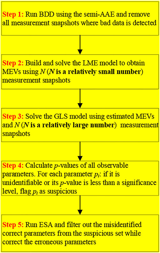
FIGURE 1. Flow chart of the proposed LME-GLS methodology.

Step 1: Bad Data Detection by Semi-AAE

Due to various disturbances in realistic power systems, it is necessary to detect bad data so as to prepare an accurate measurement dataset for subsequent PEI. In this paper, the BDD problem is viewed as a binary classification problem and solved by the semi-AAE (Makhzani et al., 2015). The semi-AAE model is designed and trained to accept each measurement snapshot as a data sample and output a detection indicator β. β = 1 indicates existence of bad data and β = 0 otherwise. The semi-supervised property makes it suitable for scenarios when only a small portion of measurement snapshots are labeled.

The AAE integrates the generative adversarial network (GAN) into the autoencoder (AE) framework. An encoder learns to convert the input data vector to a latent vector, while a decoder learns to reconstruct the original data vector from the latent vector. The aggregated posterior distribution of the latent data is defined as

$q\left(\mathit{H}\right)={\displaystyle \int q\left(\mathit{H|X}\right)p_d}\left(\mathit{X}\right)d\mathit{X}\mathrm{,}(20)$

where X is the N_m×M input data; H is the q×M latent data; q(H|X) is the encoding distribution of H given X; p_d(X) as the true distribution of X; M is the number of samples; q is the dimension of each latent vector.

AAE introduces a GAN model to regularize the aggregated posterior distribution q(H) of the latent representation to an arbitrary prior distribution p(H), such as the standard Gaussian distribution. The encoder acts as the generator of the GAN model. It tries to learn an aggregated posterior distribution q(H) to fool the discriminator of the GAN and make it falsely believe a latent vector sample comes from q(H) but is actually from p(H). The discriminator D_Gauss, on the other side, tries to classify the input samples correctly. Furthermore, to make good use of the label information of the input samples for classification use, the latent vector is augmented with an additional category variable vector using one-hot format along with an additional discriminator D_Cat. Therefore, H consists of two parts: category latent data H_C and continuous latent data H_G, which are forced to approximate a binary categorical distribution Cat(2) and a standard Gaussian distribution N(0, I), respectively. In this situation, the encoder q(H_C, H_G|X) works as the generator of both GANs so that it can simultaneously predict fake category data H_C and fake continuous data H_G. The real data of the two discriminators, i.e. H_C’ and H_G’, can be randomly sampled from Cat (2) and N(0, I).

The AAE model can be trained in three stages: reconstruction stage, regularization stage and semi-supervised classification stage:

1) In the reconstruction stage, the AE updates its encoder q(H_C, H_G|X) and decoder to minimize the reconstruction loss where the input is the unlabeled data. The encoder maps the input data X to the representation H of the hidden layer:

${\mathit{h}}_i=f\left({\mathit{x}}_i\right)=s\left(\mathit{W}{\mathit{x}}_i+\mathit{b}\right),(21)$

where h_i is the ith column vector of H; x_i is the ith column vector of X; W is the q×N_m weight matrix; b is the q × 1 offset vector; s(·) is a nonlinear activation function. The model parameters of the encoder are expressed as θ = {W,b}.

The decoder maps the latent data H to the reconstructed data X′ through the mapping function $f^{\prime }$:

${\mathit{x}}_i^{\mathit{\prime }}\mathit{=}{\mathit{f}}^{\mathit{\prime }}\left({\mathit{h}}_i^{\prime }\right)\mathit{=s}\left({\mathit{W}}^{\mathit{\prime }}{\mathit{h}}_i\mathrm{+}{\mathit{b}}^{\mathit{\prime }}\right)\mathrm{,}(22)$

where x_i′ is the ith column vector of X′; W′ is the N_m×q weight matrix; b′ is the N_m×1 offset vector. The model parameters of the decoder are expressed as θ' = {W′,b′}.

The reconstruction error Loss_R is minimized to obtain the optimized parameters:

$\underset{\mathit{\theta },{\mathit{\theta }}^{\mathit{\prime }}}{\min }Los{s}_R=\frac{1}{N}{\Vert \mathit{X}-X^{\prime }\Vert }^2(23)$

2) In the regularization stage, the discriminator parameters of the GAN models are updated first, and then the generator parameters are updated. The discriminator should distinguish real samples from fake samples as much as possible, while the generator tries to generate fake data similar to the real samples to deceive the discriminator, resulting in a two-player min-max game formulated as

$\begin{array}{l}\underset{G}{\min }\underset{D_{\text{Cat}}}{\max }{E}_{{\mathit{H}}_{\mathit{C}}^{\mathit{\prime }}\sim \text{Cat}\left(2\right)}\left[\log D_{\text{Cat}}\left({\mathit{H}}_{\mathit{C}}^{\mathit{\prime }}\right)\right]+E_{{\mathit{H}}_{\text{C}}\sim p\left({\mathit{H}}_{\text{C}}\right)}\left[\log \left(1-D_{\text{Cat}}\left(G\left({\mathit{H}}_{\text{C}}\right)\right)\right)\right]\\ \underset{G}{\min }\underset{D_{\text{Gauss}}}{\max }{E}_{{\mathit{H}}_{\mathit{G}}^{\mathit{\prime }}\sim N\left(\mathbf{0},\mathit{I}\right)}\left[\log D_{\text{Gauss}}\left({\mathit{H}}_{\mathit{G}}^{\mathit{\prime }}\right)\right]+E_{{\mathit{H}}_{\text{G}}\sim p\left({\mathit{H}}_{\text{G}}\right)}\left[\log \left(1-D_{\text{Gauss}}\left(G\left({\mathit{H}}_{\text{G}}\right)\right)\right)\right]\end{array}(24)$

where E is the expectations under a distribution; p(H_C), p(H_G) are the prior distributions of H_C, H_G; G(·) is a function mapping samples from the prior distributions to the latent data space; D_Cat(·) is a function which returns the probability that the input sample comes from the real categorical distribution Cat(2) (positive samples), rather than from our generative model (negative samples); D_Gauss(·) is a function which returns the probability that the input sample comes from the real standard Gaussian distribution N(0, I) (positive samples), rather than from our generative model (negative samples).

3) Finally, in the semi-supervised classification stage, the encoder q(H_C|X) is updated only by using the labeled data to minimize the cross-entropy loss, which is expressed as

$\underset{\mathbf{\theta }}{\min }Los{s}_S=E_{q\left({\mathit{H}}_{\text{C}}\right)}\left[-\log p\left({\mathit{H}}_{\text{C}}\right)\right](25)$

where q(H_C) is an aggregated posterior distribution of H_C.

Step 2: MEV Estimation by Solving the LME Model

Using the clean measurement dataset without outliers, the LME method presented in The LME Method for Estimation of MEVs Section is then used to estimate MEVs.

Step 3: Parameter Error Estimation by the GLS Method

Using the clean measurement dataset without outliers, the LME method is then used to estimate MEVs. Once the statistical properties of the measurement errors are estimated, then we have ${\mathbf{r}}_i\sim \left({\mathit{X}}_i{\mathit{p}}_e,{\widehat{\sigma }}^2\left(\mathit{I}+{\mathit{Z}}_i\widehat{\mathit{\Psi }}{\mathit{Z}}_i^T\right)\right)$. As follows from the Gauss-Markov theorem, p_e can be estimated directly by the GLS method:

${\widehat{\mathit{p}}}_e={\left[{\displaystyle \sum _{i=1}^N{\mathit{X}}_i^{\text{T}}{\left(\mathit{I}+{\mathit{Z}}_i\widehat{\mathit{\Psi }}{\mathit{Z}}_i^{\text{T}}\right)}^{-1}{\mathit{X}}_i}\right]}^{-1}\left[{\displaystyle \sum _{i=1}^N{\mathit{X}}_i^{\text{T}}{\left(\mathit{I}+{\mathit{Z}}_i\widehat{\mathit{\Psi }}{\mathit{Z}}_i^{\text{T}}\right)}^{-1}{\mathit{y}}_i}\right](26)$

As can be seen from (26), the GLS only involves inversion of low-dimension matrices, which is very efficient even a large number of measurement snapshots are used.

Step 4: Suspicious Parameter Selection by Hypothesis Testing

Although p_e can be estimated through GLS, the estimated ${\widehat{\mathbf{p}}}_e$ is not suitable for parameter correction as ${\widehat{\mathbf{p}}}_e$ will have many nonzero elements, even elements corresponding to correct parameters may be relatively large due to measurement noise, and the optimal solution will show some amount of “overfitting”. Therefore, ${\widehat{\mathbf{p}}}_e$ is only used for hypothesis testing to test whether each parameter error is zero or not.

The covariance matrix of ${\widehat{\mathit{p}}}_e$ can be calculated by

$\mathit{C}={\widehat{\sigma }}^2{\left[{\displaystyle \sum _{i=1}^N{\mathit{X}}_i^{\text{T}}{\left(\mathit{I}+{\mathit{Z}}_i\widehat{\mathit{\Psi }}{\mathit{Z}}_i^{\text{T}}\right)}^{-1}{\mathit{X}}_i}\right]}^{-1}.(27)$

The ith component of normalized ${\widehat{\mathbf{p}}}_e$ approximately follows a t-distribution with N_T-N_p degrees of freedom (Pinheiro and Bates, 2000):

${\gamma }_i={\widehat{p}}_{e,i}/\sqrt{C_{ii}}\sim t\left(N_T-N_p\right),(28)$

where γ_i is the t-statistic of the ith parameter error; C is the N_p×N_p covariance matrix of ${\widehat{\mathbf{p}}}_e$; C_ii is the ith diagonal element of C; N_T is the number of total measurements, N_T = NN_m.

The hypothesis testing identification (HTI) is then used to decide if a parameter is erroneous. The null hypothesis and alternative hypothesis are chosen as follows:

$H_0:p_{e,i}=0,H_1:p_{e,i}\ne 0.(29)$

The statistical significance of the ith parameter error can be tested by its two-sided p-value:

$p{-\text{value}}_i=P\left(\text{|}{\gamma }_i\text{|}<t_{\alpha /2,N_T-N_p}\right),(30)$

where t_α/2,d is the (1-α/2)th quantile of the t-distribution with d degrees of freedom, which indicates the probability of obtaining a value γ_j more extreme than the critical value. p-values below the significance level provide strong evidence for rejecting the null hypothesis.

Step 5: Parameter Correction by the ESA Method

The HTI may make two types of errors known as type I errors and type II errors. A type I error is the rejection of H₀ when it is indeed true. It is also referred to as a “false alarm” because correct parameters are misidentified as erroneous. To this end, the ESA method (Liang et al., 2021) is further used to move misidentified but correct parameters from the suspicious parameter set back to the correct parameter set while correcting the identified erroneous parameters.

Comparison With Existing Methods

The proposed method seems similar to the traditional RSA method (Liu et al., 1992; Liu and Lim, 1995). However, there are two differences between the LME-GLS method and the RSA method.

1) The RSA method is used to estimate parameter errors whereas the LME-GLS method is used to identify parameter errors. Due to different measurement configurations, measurement noise levels, and limited number of measurement snapshots used, it is possible to modify the existing values in the database, even when they are correct. On the contrary, in the LME-GLS method, only a limited number of parameters with strong evidence by data that they are undoubtedly erroneous are selected for estimation, which avoids modifying existing values to any false values as much as possible.

2) The RSA method formulates a linear model linking the residuals and the unknown parameter errors and assumes the measurement noise has a known statistic property. However, the proposed LME-GLS method formulates the residual equation as an LME model in which parameter errors and measurement noise are viewed as fixed effects and random effects, respectively. The parameter errors and variances in the measurement noise are simultaneously estimated from longitudinal residual data, followed by an HTI process.

The proposed method although cannot handle bad data directly, it makes use of a novel learning-based BDD method to guarantee only measurement snapshots that are free of any bad data are used. The comparison of the proposed learning-based bad data detection (BDD) method with classic BDD method, i.e. the Chi-squares test method using objective function values of state estimation, or the largest normalized residual (LNR) method, are summarized as follows:

1) Classic BDD methods are able to detect single bad data or multiple non-interacting bad data. However, they are incapable of detecting multiple interacting bad data whose residuals are masked by each other and the objective function value or their (normalized) residuals are smaller than the threshold even they exist. Note that the famously known false data injection attack is a special type of multiple interacting bad data, where hackers can circumvent the BDD module by tampering with the sensor measurements and injecting the elaborately designed false data without being detected.

2) Classic BDD methods depends on convergence of SE algorithms, which may be time-consuming or hard to converge, especially for large scale systems. On the other side, the learning-based BDD method is free of convergence problems and is very fast once it is well trained. In the meantime, it is very effective and can achieve very high accuracy, taking advantage of the strong feature extraction ability of neural networks.

Simulation Results

In this section, thorough tests on a large number of scenarios are provided to show the effectiveness of the proposed methodology. Multiple measurement snapshots are generated by varying the loading condition between approximately 0.8 and 1.2 times their nominal values using MATPOWER (Zimmerman et al., 2011). The measurements are divided into five groups: real power flow measurements (PF), real power injection measurements (PI), reactive power flow measurements (QF), reactive power injection measurements (QI), voltage magnitude measurements (VM), and different levels of measurement noise are used for each group. The selected line parameters are added with an error value of +30%. The significance level for the p-values is set to 0.05.

BDD Results

In this section, the IEEE 14-bus system is used to test the effectiveness of the semi-AAE-based BDD method in the presence of erroneous parameters and limited labels. There are 20 series branches (transmission lines and transformers) and 40 series parameters (resistances and reactances) in this system. +30% relative error are added to parameters r_2-4, r_2-5, r_3-4 and r_4-5. Full measurement configuration is assumed. Relative measurement errors are added to the true values of measurements by z_i = z_i,true×(1 + e_type×σ) where z_i, z_i,true are measured and true value of measurement i, e_type is percent relative error corresponding to measurement i’s type, σ is a random variable obeying standard Gaussian distribution. Measurement errors are set as e_PF = e_QF = 0.5%, e_PI = e_QI = 1.0%, e_VM = 0.2%. Monte Carlo simulation is used to generate 5000 normal measurement snapshots without bad data. Relatively large errors (10–20% of the normal values) are added to 8–12% of measurements in each measurement snapshot to generate another 5000 measurement snapshots with bad data. 80% of the whole 10,000 measurement snapshots are selected as the training dataset and the left 20% as the testing dataset. Only 10% of all snapshots are labeled β = 0 or 1, including 500 normal measurement snapshots with label β = 0 and 500 erroneous measurement snapshots with label β = 1, respectively. The performance of the semi-AAE method is evaluated by the following accuracy rate (A), which refers to the percentage that the detection results are correct among the prediction results of all samples:

$A=\frac{TP+TN}{TP+TN+FP+FN},(31)$

where TP means true positive, TN means true negative, FP means false positive, and FN means false negative. Their specific definitions are shown in Table 1.

TABLE 1

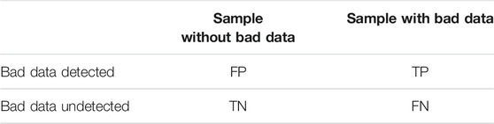
TABLE 1. Definitions of the four statistics indices.

The accuracy, detection time and training time are shown in Table 2. It can be seen that the detection accuracy on the training set and testing set reach 96.5 and 94.5%, respectively, showing that the algorithm is effective for BDD. At the same time, the training time is only 124.38 s, and the detection time is only 0.66 s, which shows that the AAE can meet the requirements of online BDD.

TABLE 2

TABLE 2. BDD performance of the semi-AAE method on the IEEE 14-bus system.

PEI Results

The IEEE 14-Bus System

In this section, the IEEE 14-bus system is used to test the effectiveness of the proposed PEI method. Let measurement redundancy be defined as η = N_m/N_s. For the IEEE 14-bus system, the following cases are designed:

Case 1: e_PF = e_QF = 0.5%, e_PI = e_QI = 1.0%, e_VM = 0.2%, η = 4.52.

Case 2: e_PF = e_QF = 1.0%, e_PI = e_QI = 1.5%, e_VM = 0.5%, η = 4.52.

Case 3: e_PF = e_QF = 0.5%, e_PI = e_QI = 1.0%, e_VM = 0.2%, η = 3.04.

Case 4: e_PF = e_QF = 1.0%, e_PI = e_QI = 1.5%, e_VM = 0.5%, η = 3.04.

In Case 1 and Case 2, full measurement redundancy is assumed, resulting in a high η value. In Case 3 and Case 4, we delete all the real/reactive power flow measurements at the end of each branch, resulting in a lower η value.

Different combinations of erroneous parameters are simulated to test the performance of the proposed methodology. If N_e parameter errors are assumed to exist, then there will be $C_{N_p}^{N_e}$ different combinations of erroneous parameters, among which 100 combinations are selected for testing. In the LME step (Step 2 in Figure 1), N_LME measurement snapshots are used to test the estimation accuracy of the MEVs and its impact on the whole success rate. In the GLS-HTI step (Step 3-4 in Figure 1), maximally 100 measurement snapshots (N_GLS = 10, 20, … , 100) are used for parameter error estimation and hypothesis testing.

Simulation results show that three snapshots are enough to obtain acceptable MEVs. The estimated MEVs of the four cases when N_LME = 3 are summarized in Table 3. If larger N_LME is used, the estimated MEVs only slightly differ from the current values but much heavier computation burden is needed.

TABLE 3

TABLE 3. Estimated MEVs of the IEEE 14-bus system (N_LME = 3).

Then, based on the estimated MEVs in Table 3, the GLS is carried out to test the success rates of PEI. For each PEI test, the result is defined as “success” if all the erroneous parameters’ p-values rank top k ones among the whole N_p parameters’ p-values sorted in ascending order. k = min(N_max, N_threshold), where N_max is a constant depending on N_e (N_max = 2N_e in this paper), N_threshold is the number of parameters whose p-values are smaller than a predefined significance level (0.05 through all simulations). In this way only N_max parameters are selected as suspicious if a large number of parameters fail the hypothesis testing and thus the maximum number of suspicious parameters can be controlled.

The success rate results of the four cases are shown in Figures 2A–D respectively, where N_e can be 2, three or 4. It can be seen that the success rates increase with increasing measurement snapshots. For Case 1 with the highest measurement accuracy and the largest measurement redundancy, Figure 2A shows that when the number of measurement snapshots N is 10, the minimum success rate is only about 60%. However, when the number of measurement snapshots is 20, the success rate reaches above 90%. By increasing N, the success rates can be higher than 95%, or even 100%. For Case 2 with the same redundancy and lower measurement accuracy, Figure 2B shows that the minimum success rate is only 33% when N is 10. As N increases, the success rate also gradually increases, but the final result is less than 100%. For Case 3 with high precision and low redundancy, Figure 2C shows that when N is 10, the minimum success rate is only 38%, but with the increase of N, the success rate gradually increases and can reach 100%. Finally for Case 4 with lowest measurement accuracy and redundancy, Figure 2D shows that the minimum success rate reduces to 10% when N is 10, and the highest success rate is only 82% when N increase to 100.

FIGURE 2

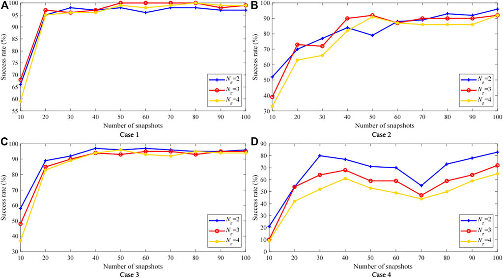
FIGURE 2. PEI success rate of the IEEE 14-bus system.

Comparing the results of Case 1–4 in Figure 2, it can be seen that the accuracy of measurements has a great impact on the performance of the PEI method proposed in this paper, while the measurement redundancy has less impact on this method. In addition, the success rates gradually increase with the increase of the number of measurement snapshots used.

Figure 3 shows the success rates of PEI using empirical values of MEVs, taking Case 1 as an example, i.e. e_PF = e_QF = 0.005 p.u., e_PI = e_QI = 0.010 p.u., e_VM = 0.002 p.u. It can be seen that the maximum success rate is only 85%. Compared with Figure 2A, the maximum decline of success rate is more than 20%, and the success rate become lower when more parameter errors exist, which verifies the advantages of using the LME model to estimate the MEVs.

FIGURE 3

FIGURE 3. PEI success rate of the IEEE 14-bus system using empirical MEVs (Case 1).

The IEEE 30-Bus System

In this section, the IEEE 30-bus system is used to test the effectiveness of the proposed PEI method. There are 41 series branches and 82 series parameters in this system. As the true values of the loads and power flow are very small for this system, small absolute errors for measurements are added. The following cases are designed:

Case 1: e_PF = e_QF = 0.3%, e_PI = e_QI = 0.5%, e_VM = 0.2%, η = 4.31.

Case 2: e_PF = e_QF = 0.3%, e_PI = e_QI = 0.5%, e_VM = 0.2%, η = 2.92.

Similarly, 100 different error parameter combinations are selected to test the performance of the proposed method. The estimated MEVs of the two cases are summarized in Table 4. Then, based on the estimated MEVs in Table 4, the GLS is carried out for PEI. For Case 1, one scenario (N_e = 6) is randomly selected from 100 combinations and the p-values of all 82 line parameters using 10–100 snapshots are shown in Figure 4. It can be seen that all erroneous parameters except for r_3-4 are identified. The erroneous parameter r_3-4 is missed because the resistance value of this line is too small and the objective function has low sensitivity to it.

TABLE 4

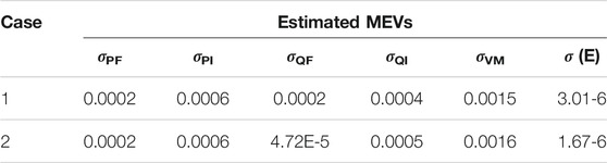
TABLE 4. Estimated MEVs of the IEEE 30-bus system (N_LME = 3).

FIGURE 4

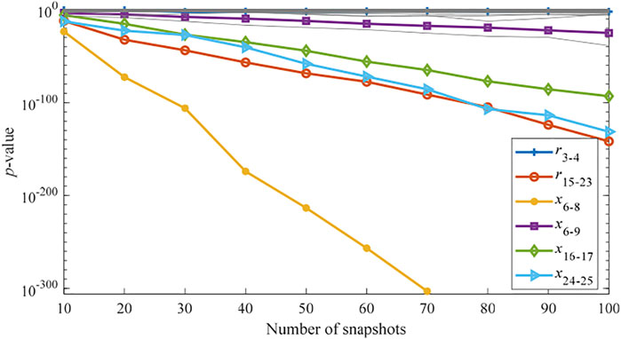
FIGURE 4. p-values of all parameters in the IEEE 30-bus system (Case 1, N_e = 6).

The success rate results of the two cases using at most 100 snapshots are shown in Figure 5, where N_e can be 2, 3, 4, 5 or 6. For Case 1, Figure 5A shows that the success rate increases if more measurement snapshots are used from the overall perspective. Specifically, when 100 snapshots are used, all the success rates of PEI are above 95%. For Case 2 with high precision but low redundancy, Figure 5B shows the success rate is greatly affected. When 10 measurement snapshots are used, the minimum success rate is only 11% (N_e = 6), and the highest success rate is only 48% (N_e = 2). In addition, the success rate does not show a monotonous increase as N increases. When N is 100, mostly success rates concentrated at 70%, which is far worse than Case 1.

FIGURE 5

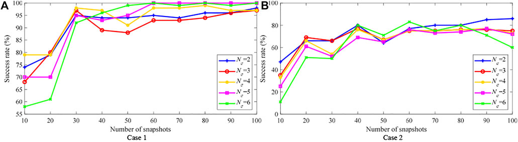
FIGURE 5. PEI success rate of the IEEE 30-bus system.

However, the PEI results show much better performance if the definition of “success” is relaxed, i.e. for each PEI test, the result is defined as “success” if all the erroneous parameters’ p-values “but one” rank top k ones among the whole N_p parameters’ p-values sorted in ascending order. In other words, missing of one erroneous parameter is permitted and still viewed as “success”. The success rates under this definition for Case 2 are shown in Figure 6. We can see much higher success rates can be achieved than in Figure 5B. For example, the success rate rises from 48 to 91% when N = 10, N_e = 6, which means that in most tests only one erroneous parameter is missed by the proposed method due to this missed parameter’s low sensitivity.

FIGURE 6

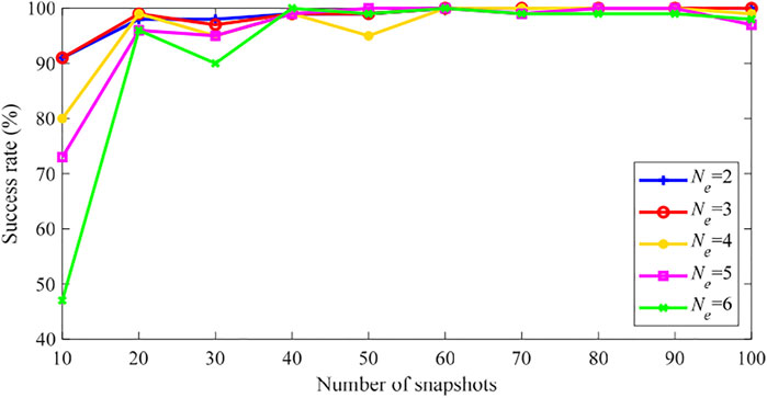
FIGURE 6. PEI success rate of the IEEE 30-bus system (Case 2, 1 missing).

Figure 7 shows the PEI results using empirical MEVs, taking Case 1 as an example. It can be seen that the success rate of PEI is less than 30% when 10 snapshots is used, and the success rate increases with the increase of N. Even when N is 100, the maximum success rate is only 65%. Compared with Figure 5A, the success rate is reduced by 30%, which proves the superiority of using LME method for MEV estimation.

FIGURE 7

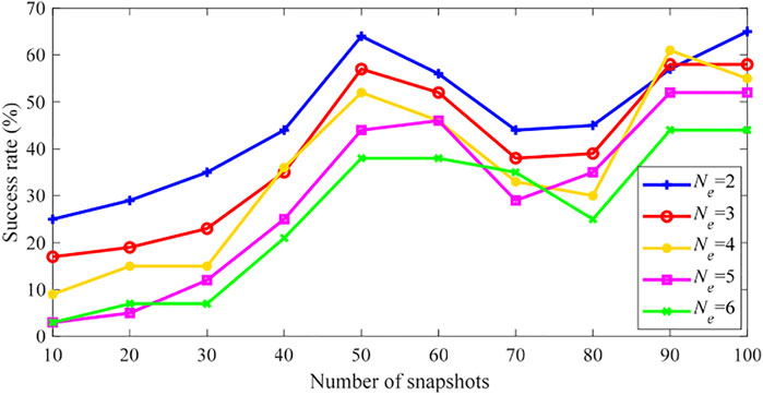
FIGURE 7. PEI success rate of the IEEE 30-bus system using empirical MEVs (Case 1).

The IEEE 118-Bus System

In this section, the proposed method is evaluated on the IEEE 118-bus system with 186 series branches and 372 series parameters. The following cases are designed for testing:

Case 1: e_PF = e_QF = 0.5%, e_PI = e_QI = 1.0%, e_VM = 0.2%, η = 4.67.

Case 2: e_PF = e_QF = 1.0%, e_PI = e_QI = 1.5%, e_VM = 0.5%, η = 4.67.

Case 3: e_PF = e_QF = 0.5%, e_PI = e_QI = 1.0%, e_VM = 0.2%, η = 3.09.

Case 4: e_PF = e_QF = 1.0%, e_PI = e_QI = 1.5%, e_VM = 0.5%, η = 3.09.

Similarly, in Case 1 and Case 2, full measurement redundancy is assumed, resulting in a high η value. In Case 3 and Case 4, we delete all the real/reactive power flow measurements at the end of each branch, resulting in a lower η value. Three measurement snapshots are used for MEV estimation, which is then used for the GLS-based PEI. The estimated MEVs of the four cases are summarized in Table 5.

TABLE 5

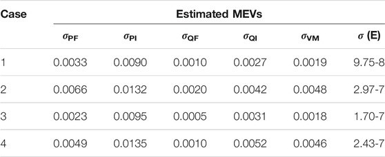
TABLE 5. Estimated MEVs of the IEEE 118-bus system (N_LME = 3).

For Case 1, one scenario (N_e = 10) is randomly selected from 100 combinations and the p-values of all 372 line parameters are shown in Figure 8. It can be seen that all the erroneous parameters rank first and are correctly identified. Note that the p-value curve of parameter x_100-103 is too small to be displayed.

FIGURE 8

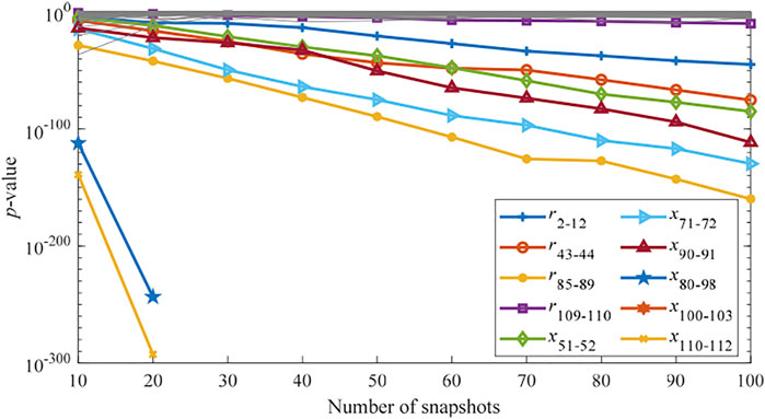
FIGURE 8. p-values of all parameters in the IEEE 118-bus system (Case 1, N_e = 10).

The success rate results of the four cases are shown in Figure 9, where N_e can be 2–10. For Case 1 and Case 3, Figures 9A,C show that even if a large number of error parameters exist, the success rates can still reach a high level as long as the measurement accuracy is high, and the success rate will gradually increase with the increase of N. For Case 2 and Case 4 with lower measurement accuracy, Figures 9B,D show that the number of successful PEI is greatly reduced, especially for Case 4 with both lower measurement accuracy and lower measurement redundancy.

FIGURE 9

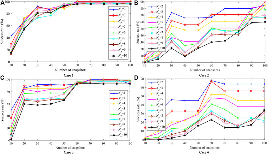
FIGURE 9. PEI success rate of the IEEE 118-bus system.

Then, if we relax the definition of “success”, i.e. missing of one or more erroneous parameter is permitted and still viewed as “success”. Figures 10, 11 show that much better performance can be achieved, compared with Figures 9B,D. This means that in most tests only one or two erroneous parameters are missed while most erroneous parameters are actually correctly identified by the proposed method.

FIGURE 10

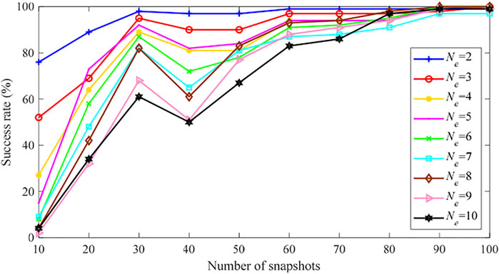
FIGURE 10. PEI success rate of the IEEE 118-bus system (Case 2, 1 missing).

FIGURE 11

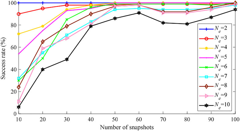
FIGURE 11. PEI success rate of the IEEE 118-bus system (Case 4, 2 missing).

Figure 12 shows the success rates of PEI using empirical MEVs taking Case 1 as an example. By comparing the results of Figure 9A and Figure 12, it can be concluded that the MEVs estimated by solving the LME model result in much better PEI performance than empirical ones.

FIGURE 12

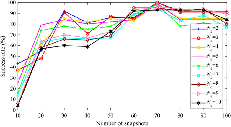
FIGURE 12. PEI success rate of the IEEE 118-bus system using empirical MEVs (Case 1).

Computation Time

All the tests above are performed on a personal computer with a 3.70 GHz i7-8700K CPU and 32 GB RAM. Table 6 shows the computation times of different methods under different scenarios. It can be seen that the proposed LME-GLS method greatly saves the calculation time than the original LME-based PEI method. The main reason is that this method only uses a small number of measurement snapshots to estimate the MEVs, which avoids the computational burden of solving a very large-scale LME model. In addition, the GLS only involves inversion of low-dimension matrices thus is very fast without losing the PEI accuracy.

TABLE 6

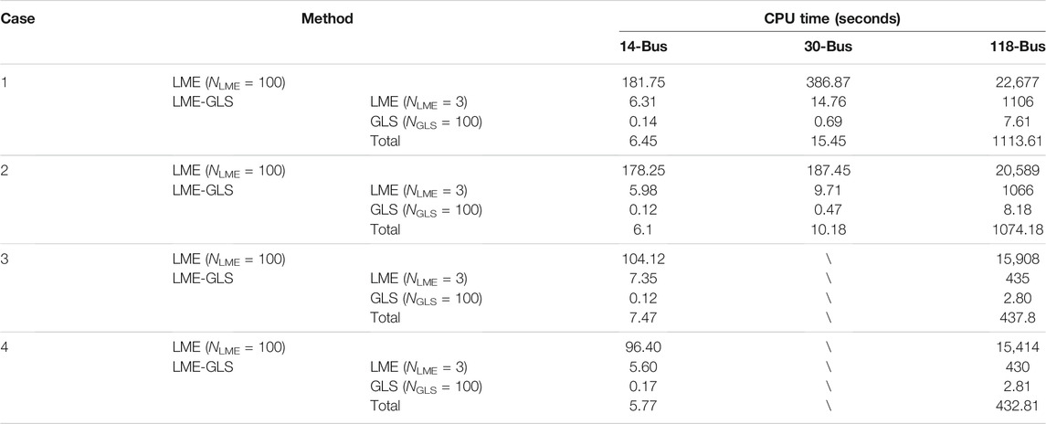
TABLE 6. CPU time comparison.

Conclusion

This paper proposes an efficient method for the simultaneous identification of multiple network parameter errors based on an LME model and the GLS method. The residual equations from multiple-snapshot state estimation are used to formulate the LME model in which the parameter errors are considered as the fixed effects and the measurement errors are considered as the random effects. Then, using the measurement error variances estimated by solving the LME model, the GLS is used to estimate the parameter errors along with a hypothesis testing to infer whether each parameter error is zero. The key advantage of the proposed methodology lies in that the LME model is only used to estimate the variances of the measurement errors using a small number of measurement snapshots, therefore the huge computation burden needed to solve a large-scale LME model is avoided. In addition, the GLS only involves inversion of low-dimension matrices, which is very efficient even a large number of measurement snapshots are used.

The proposed method is shown to be promising for the simultaneous identification of multiple parameter errors. It can be used periodically by system operators in an offline manner using multiple measurement snapshots, to identify and correct multiple erroneous parameters once large residuals are reported by state estimator and existence of parameter errors are suspected. However, parameter errors are treated as unknown constants in this paper rather than random variables. Considering continuous varying of parameters during various operating conditions and load levels, future work will be focused on dynamic parameter tracking using phasor measurements.

Data Availability Statement

The raw data supporting the conclusion of this article will be made available by the authors, without undue reservation.

Author Contributions

DL contributed toward supervision, conceptualization, and writing—review and editing. YC contributed toward methodology, software, data curation, and writing—original draft. SS contributed toward software and data curation. XW contributed toward writing—review and editing. LZ contributed toward writing—review and editing.

Funding

This work is supported by the Natural Science Foundation of Hebei Province of China under Grant E2021202053, the Natural Science Foundation of the Department of Education of Hebei Province of China under Grant QN2020442, the China Postdoctoral Science Foundation under Grant 2019M660966, and State Key Laboratory of Reliability and Intelligence of Electrical Equipment (Hebei University of Technology) under Grant EERI_PI2020002.

Conflict of Interest

The authors declare that the research was conducted in the absence of any commercial or financial relationships that could be construed as a potential conflict of interest.

Publisher’s Note

All claims expressed in this article are solely those of the authors and do not necessarily represent those of their affiliated organizations, or those of the publisher, the editors and the reviewers. Any product that may be evaluated in this article, or claim that may be made by its manufacturer, is not guaranteed or endorsed by the publisher.

Acknowledgments

The authors would like to thank the financial support received from the Natural Science Foundation of Hebei Province of China, the Natural Science Foundation of the Department of Education of Hebei Province of China, the China Postdoctoral Science Foundation, and State Key Laboratory of Reliability and Intelligence of Electrical Equipment (Hebei University of Technology). We would like to thank the reviewers for their valuable comments.

References

Abur, A., and Gómez-Expósito, A. (2004). Power System State Estimation—Theory and Implementation. New York: Marcel Dekker Press.

Google Scholar

Bates, D., Maechler, M., Bolker, B., and Walker, S. (2015). Fitting Linear Mixed-Effects Models Using Lme4. J. Stat. Soft. 67 (1), 1–48. doi:10.18637/jss.v067.i01

CrossRef Full Text | Google Scholar

Bian, X., Li, X. R., Chen, H., Gan, D., and Qiu, J. (2011). Joint Estimation of State and Parameter with Synchrophasors-Part II: Parameter Tracking. IEEE Trans. Power Syst. 26 (3), 1209–1220. doi:10.1109/tpwrs.2010.2098423

CrossRef Full Text | Google Scholar

Cain, M. B., O’neill, R. P., and Castillo, A. (2012). History of Optimal Power Flow and Formulations. Fed. Energ. Regul. Comm. 33.

Google Scholar

Castillo, M. R. M., London, J. B. A., Bretas, N. G., Lefebvre, S., Prévost, J., and Lambert, B. (2011). Offline Detection, Identification, and Correction of branch Parameter Errors Based on Several Measurement Snapshots. IEEE Trans. Power Syst. 26 (2), 870–877. doi:10.1109/TPWRS.2010.2061876

CrossRef Full Text | Google Scholar

Debs, A. (1974). Estimation of Steady-State Power System Model Parameters. IEEE Trans. Power Apparatus Syst. PAS-93 (5), 1260–1268. doi:10.1109/tpas.1974.293849

CrossRef Full Text | Google Scholar

Dobakhshari, A. S., Abdolmaleki, M., Terzija, V., and Azizi, S. (2020). Online Non-Iterative Estimation of Transmission Line and Transformer Parameters by SCADA Data. IEEE Trans. Power Syst. 36 (3), 2632–2641. doi:10.1109/TPWRS.2020.3037997

CrossRef Full Text | Google Scholar

Kusic, G. L., and Garrison, D. L. (2004). Measurement of Transmission Line Parameters from SCADA Data. IEEE Power Syst. Conf. Expo. 1, 440–445. doi:10.1109/PSCE.2004.1397479

CrossRef Full Text | Google Scholar

Liang, D., Zeng, L., and Chiang, H.-D. (2021). Simultaneous Identification and Correction of Multiple Network Parameter Errors by Mixed-Effects Models. IEEE Trans. Control. Netw. Syst., 1. doi:10.1109/TCNS.2021.3124899

CrossRef Full Text | Google Scholar

Lin, Y., and Abur, A. (2018). A New Framework for Detection and Identification of Network Parameter Errors. IEEE Trans. Smart Grid 9 (3), 1698–1706. doi:10.1109/tsg.2016.2597286

CrossRef Full Text | Google Scholar

Lin, Y., and Abur, A. (2017). Enhancing Network Parameter Error Detection and Correction via Multiple Measurement Scans. IEEE Trans. Power Syst. 32 (3), 2417–2425. doi:10.1109/tpwrs.2016.2608964

CrossRef Full Text | Google Scholar

Liu, W.-H. E., and Lim, S. L. (1995). Parameter Error Identification and Estimation in Power System State Estimation. IEEE Trans. Power Syst. 10 (1), 200–209. doi:10.1109/59.373943

CrossRef Full Text | Google Scholar

Liu, W.-H. E., Wu, F. F., and Lun, S.-M. (1992). Estimation of Parameter Errors from Measurement Residuals in State Estimation (Power Systems). IEEE Trans. Power Syst. 7 (1), 81–89. doi:10.1109/59.141690

CrossRef Full Text | Google Scholar

Makhzani, A., Shlens, J., Jaitly, N., Goodfellow, I., and Frey, B. (2015). Adversarial Autoencoders. [Online] Available: https://arxiv.org/abs/1511.05644.

Google Scholar

Monticelli, A. (1999). State Estimation in Electric Power Systems: A Generalized Approach. Norwell, MA, USA: Kluwer Press.

Google Scholar

Pinheiro, J. C., and Bates, D. (2000). Mixed-Effects Models in S and S-PLUS. Berlin: Springer-Verlag Press.

Google Scholar

Ren, P., Lev-Ari, H., and Abur, A. (2017). Tracking Three-Phase Untransposed Transmission Line Parameters Using Synchronized Measurements. IEEE Trans. Power Syst. 33 (4), 4155–4163. doi:10.1109/TPWRS.2017.2780225

CrossRef Full Text | Google Scholar

Slutsker, I. W., Mokhtari, S., and Clements, K. A. (1996). Real Time Recursive Parameter Estimation in Energy Management Systems. IEEE Trans. Power Syst. 11 (3), 1393–1399. doi:10.1109/59.535680

CrossRef Full Text | Google Scholar

Wang, Y., Xu, W., and Shen, J. (2015). Online Tracking of Transmission-Line Parameters Using SCADA Data. IEEE Trans. Power Deliv. 31 (2), 674–682. doi:10.1109/TPWRD.2015.2474699

CrossRef Full Text | Google Scholar

Williams, T. L., Sun, Y., and Schneider, K. (2016). Off-Line Tracking of Series Parameters in Distribution Systems Using AMI Data. Electric Power Syst. Res. 134, 205–212. doi:10.1016/j.epsr.2015.12.036

CrossRef Full Text | Google Scholar

Zarco, P., and Exposito, A. G. (2000). Power System Parameter Estimation: A Survey. IEEE Trans. Power Syst. 15 (1), 216–222. doi:10.1109/59.852124

CrossRef Full Text | Google Scholar

Zhang, L., and Abur, A. (2013). Identifying Parameter Errors via Multiple Measurement Scans. IEEE Trans. Power Syst. 28 (4), 3916–3923. doi:10.1109/tpwrs.2013.2254504

CrossRef Full Text | Google Scholar

Zhao, J., Fliscounakis, S., Panciatici, P., and Mili, L. (2018). Robust Parameter Estimation of the French Power System Using Field Data. IEEE Trans. Smart Grid 10 (5), 5334–5344. doi:10.1109/tsg.2018.2880453

CrossRef Full Text | Google Scholar

Zhao, J., Qi, J., Huang, Z., Meliopoulos, A. P. S., Gomez-Exposito, A., Netto, M., et al. (2019). Power System Dynamic State Estimation: Motivations, Definitions, Methodologies, and Future Work. IEEE Trans. Power Syst. 34 (4), 3188–3198. doi:10.1109/tpwrs.2019.2894769

CrossRef Full Text | Google Scholar

Zhu, J., and Abur, A. (2006). Identification of Network Parameter Errors. IEEE Trans. Power Syst. 21 (2), 586–592. doi:10.1109/tpwrs.2006.873419

CrossRef Full Text | Google Scholar

Zimmerman, R. D., Murillo-Sánchez, C. E., and Thomas, R. J. (2011). MATPOWER: Steady-State Operations, Planning, and Analysis Tools for Power Systems Research and Education. IEEE Trans. Power Syst. 26 (1), 12–19. doi:10.1109/TPWRS.2010.2051168

CrossRef Full Text | Google Scholar